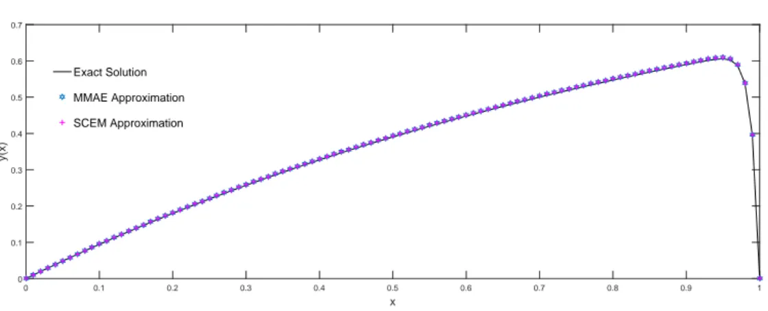
A comparison between MMAE and SCEM for solving singularly perturbed linear boundary layer problems
Tam metin
Şekil

Benzer Belgeler
Names are the very stuff of prosopography: without a knowledge of anthro— ponymic information, the prosopographer would be unable to identify and distinguish between individuals in
Working in an environment with people from different countries or teaching students with different cultures had positive impacts on the way teachers facilitate learning in
Sonuç olarak bu çalışmada yerli kahverengi yumurtacı ATAK ve ATAK-S hibritlerin performanslarının dış kaynaklı hibritlere göre özellikle yumurta verimi ve yem
All in all, by combining the reconstructed disk distribution of active regions with their brightness contrasts, we generated light curves with a time span of 310 years as they would
homeostazisinin düzenlenmesinde etkin bir rol oynamaktadır [11]. Bu etkisini ağırlıklı olarak G-proteini ve PKA aracılığıyla SR üzerinde bulunan RYR ve SERCA kanal
SUMMARY This case report aimed to describe the fabrication procedure and treatment efficacy of an individual, one-piece, non-adjustable mandibular advancement device (MAD) for
Her bir hareket ic¸in ayrı ayrı ve rasgele sec¸ilmis¸ olan 24’er tane ¨oznitelik vekt¨or¨un¨un ortalaması alınarak 8 farklı hareket ic¸in birer tane e˘gitme vekt¨or¨u
Alkol kullanan kişilerde herhangi bir karaciğer hastalığı yokluğunda, GGT düzeyindeki bir artışın ‘alkol suistimalinin erken uyarıcısı’ olarak yorumlanmasının daha
