AN ANALYSIS OF WAGE, EARNINGS AND
INCOME INEQUALITY IN TURKEY
Graduate School of Social Sciences
TOBB University of Economics and Technology
EMRE BİLAL ARSLAN
In Partial Fulfillment of the Requirements for the Degree
of
Master of Science
in
THE DEPARTMENT OF ECONOMICS
TOBB UNIVERSITY OF ECONOMICS AND TECHNOLOGY
ANKARA
iv
ABSTRACT
AN ANALYSIS OF WAGE, EARNINGS AND
INCOME INEQUALITY IN TURKEY ARSLAN, Emre Bilal
M.Sc., Department of Economics Supervisor: Assist. Prof. Ozan Ekşi
February 2014
The goal of this thesis is to analyze wage, income, and earnings inequalities in Turkey by using the data from Household Budget Surveys that have been available yearly since 2002. A thorough documentation of earnings and hourly wage inequalities is provided for different education and experience groups. The study then documents income inequality in Turkey. Both household and individual income data are used. The importance of household data arises from the fact that the members of a household use the same income sources, and social planners recognize this fact in calculating the well-being of their citizens. Therefore, the difference between household and individual income distributions is important to show the within-country income sharing dynamics in Turkey. Next, a decomposition of yearly incomes to earnings and non-earnings income sources is provided, together with figures showing the distribution of these income sources across households. The second part of the thesis explains the changes in income inequality in Turkey through panel regressions by using the cohort inequality indices.
v
Briefly, this thesis aims to make a significant contribution to the literature and to create an important source of information. The most remarkable results are: the annual earning inequality differs from hourly wage inequality in Turkey.
The 2001 crisis had a significant effect on inequality especially during the period of 2002-2004. Earnings are the most important source of individual income and the distribution of earnings and non-earnings does not change significantly over the years. With regard to the results obtained through panel regressions, the most influential variable that changes inequality between 2002 and 2011 is the ratio of credit to the private sector by deposit money banks and other financial institutions to GDP. This variable is used as a financial depth indicator and has an increasing effect on inequality.
JEL Codes: D31
vi
ÖZET
TÜRKİYE’ DEKİ ÜCRET, KAZANÇ VE
GELİR DAĞILIMI EŞİTSİZLİĞİNİN ANALİZİ
ARSLAN, Emre Bilal Yüksek Lisans, Ekonomi Bölümü Tez Yöneticisi: Yrd. Doç. Dr.Ozan Ekşi
Şubat 2014
Bu tezde Türkiye’deki ücret, gelir ve kazanç eşitsizliğinin analizi yapılmıştır. Veri seti olarak Devlet İstatistik Enstitüsünün (DİE, yeni adıyla Türkiye İstatistik Kurumu; TÜİK) 2002 yılından itibaren yıllık olarak yürüttüğü Hane halkı Bütçe Anketleri kullanılmıştır. Türkiye’deki ücret ve gelir eşitsizliğinin ayrıntılı incelenmesi farklı eğitim ve iş tecrübesi grupları için yapılmıştır. Yine veri olarak hem birey gelir verisi, hem de hane halkı gelir verisi kullanılmıştır. Hane halkı gelirlerinin kullanılmasının sebebi, bu gruba ait kişilerin ortak bir gelire sahip olmaları ve sosyal planlayıcının bu kişilerin refahını ölçerken bu gerçeği dikkate almasıdır. Dolayısıyla hane halkı ve birey gelir dağılımları arasındaki fark, ülke içindeki gelir paylaşım dinamiklerini göstermesi sebebiyle önem teşkil etmektedir. Bu dinamikler, Türkiye sosyal yapısı itibariyle birey gelirlerinin geniş hane halkları tarafından paylaşıldığı bir ülke olduğundan, örneğin Avrupa ülkeleri ile farklılık gösterebilecektir.
Daha sonra, yıllık gelirlerin emek ve emek dışı gelir kaynakları ile dekompozisyonu yapılmıştır ve bu gelir kaynaklarının hane halkı üzerindeki dağılımı gösterilmiştir.
vii
Diğer bulgular ise kısaca şu şekilde özetlenebilir: Türkiye’ de yıllık ücret eşitsizliği, saatlik kazanç eşitsizliğine göre farklılıklara sahiptir. Özellikle 2002 ile 2004 arasındaki periyotta 2001’de yaşanan ekonomik kriz eşitsizlik üzerinde önemli bir etkiye sahiptir. Fert gelirlerindeki en önemli kalemi çalışarak elde edilen kazanç oluşturmaktadır. Ayrıca emek ve emek dışı elde edilen kazanç dağılımları yıllara göre değişkenlik göstermemektedir.
Tezin ikinci kısmında Türkiye’deki gelir eşitsizliğini açıklayıcı değişkenler zaman serisi kullanan regresyonlar yardımıyla açıklanmıştır. Regresyonlar sonucu elde edilen bulgulara göre ise, 2002 ile 2011 yılları arasındaki periyotta gelir eşitsizliği üzerindeki en etkili değişken, mevduat bankaları ve diğer mali kurumlar tarafından özel sektöre sağlanan kredilerin GSYH (Gayri Safi Yurtiçi Hasıla)‘ya oranıdır. Bu değişken, bir finansal derinlik göstergesi olarak kullanılmaktadır ve eşitsizlik üzerinde artan bir etkisi vardır.
viii
ACKNOWLEDGMENTS
I would like to express my special appreciation and thanks to my advisor, Asst. Prof. Ozan Ekşi: you have been a tremendous guide for me and this thesis would not have been possible without your help.
I would also like to thank my committee members, Assoc. Prof. Güldem Ökem and Asst. Prof. Ünay Tamgaç Tezcan for letting my defense be an enjoyable moment, and for giving me constructive comments and warm encouragement.
In addition, I owe a very important debt to Prof. Hüseyin Merdan for his endless assistance to me in any case from the beginning of my undergraduate years till the end.
I offer my intellectual debt and special gratitude to Prof. Zeynep Aycan, for her unforgettable mentorship. I would not be able to survive in the academic community without her support.
I thank TOBB ETÜ, Department of Economics and Koç University, MA in Economics for providing me academic and financial support.
I would also like to thank all of my friends who supported me in writing, and gave me the incentive to strive towards my goal.
My deepest appreciation goes to my beloved Yasemin Uğur, for her unconditional love and the sleepless nights she spent.
Last but not least, I would like to give my special thanks to my family for their endless love. Words cannot express how grateful I am for them.
ix TABLE OF CONTENTS Abstract... iv Özet... vi Acknowledgments... viii Table of Contents... ix List of Tables... xi
List of Figures... xii
Chapter One: Introduction... 1
1.1. Introduction... 1
1.2. Literature Review... 7
1.3. Data... 11
Chapter Two: Documenting Earnings, Wage, and Income Inequalities in Turkey, 2002-2011... 13
2.1. Earnings Inequality... 13
2.2. Earnings Inequality Analysis by Percentile Groups... 16
2.3. Earnings Inequality by Age... 17
2.4. Earnings Inequality by Education Level... 18
2.5. Wage Inequality: Analysis by Percentile Groups... 20
2.6. Wage Inequality by Age... 21
2.7. Wage Inequality by Education Level... 22
2.8. Income Inequality... 23
2.9. Income Inequality Analysis by Percentile Groups... 24
2.10. Income Inequality by Education Level... 27
2.11. Income Inequality by Work Experience... 28
2.12. Income Inequality by Age Groups... 30
x
2.14. Decomposition of Income Inequality... 35
2.15. Results... 37
Chapter Three: Regression Analysis of Income Inequality in Turkey, 2002-2011... 38
3.1. Cohort Income Inequalities: Panel Data Structure... 38
3.2. Analysis by Gini Index... 39
3.3. Comparison of Measures of Inequality... 41
3.4. Explanation of Income Inequality in Turkey Through Regression Analysis: Empirical Framework... 42
3.5. Variables Used in the Regression Models: Education... 45
3.6. Social Development/ Health Expenditure... 45
3.7. Income Distribution... 45
3.8. GDP (Gross Domestic Product)... 46
3.9. Trade Globalization... 46
3.10. Financial Globalization... 46
3.11. Private Credit... 47
3.12. Education... 47
3.13. Sectoral Employment... 47
3.14. Results of Regression Analysis: Fixed Effects Regression... 48
3.15. FE Regression for Model 1: Inequality Model Constructed by the Author... 48
3.16. Robustness Check for Model 1... 49
3.17. FE Regression for Model 2: IMF Model... 52
3.18. Robustness Check for Model 2... 54
Chapter Four: Conclusion... 57
xi
LIST OF TABLES
1 Decomposition of Income Inequality... 36
2 Fixed Effect Regression Results for Proposed Model... 49
3 Robustness Check, Changing the Control Variables... 51
4 Fixed Effect Regression Results for the Proposed Model... 54
5 Robustness Check, Changing the Control Variables... 56
xii
LIST OF FIGURES
1 Gini Coefficients for Annual Earnings and Hourly Wage
Rate, 2002-2011... 14 2 Log Annual Earnings Variance and its Components,
2002-2011... 15 3 Indexed Real Annual Earnings by Percentile, 2002-2011... 17 4 Log Real Annual-Earnings Changes by Percentile for Selected
Age Groups... 18 5 Log Real Annual-Earnings Changes by Percentile for
Education Groups, 2002-2011... 19 6 Indexed Real Hourly Wage Rate by Percentile, 2002-2011... 20 7 Log Real Hourly Wage Changes by Percentile for Selected
Age Groups, 2002-2011... 21 8 Log Real Hourly Wage Changes by Percentile for Education
Groups, 2002-2011... 22 9 Gini Index for Total Individual Income...…. 23 10 Gini Index for Total Household Income... 24 11 Median, 90th Percentile, and 10th Percentile Individual
Income, 2002-2011... 25 12 Median, 90th Percentile, and 10th Percentile Household
Income, 2002-2011... 26 13 Median, 90th Percentile, and 10th Percentile Individual
Income by Education Level, 2002-2011... 28 14 Median, 90th Percentile, and 10th Percentile Individual
Income by Work Experience Groups, 2002-2011... 29 15 Median, 90th Percentile, and 10th Percentile Individual
Income by Age Groups, 2002-2011... 31 16 Earnings, Non-Earnings and Total Income Distributions,
xiii
17 Earnings and Non-Earnings Income Distribution of Households,
2002 - 2005 - 2008 - 2011... 34 18 Gini Indexes Calculated for Cohorts... 40 19 Average Growth in Within-Cohort Inequality vs. Growth
1
CHAPTER ONE
INTRODUCTION
1.1. INTRODUCTION
This thesis analyzes wage, income, and earnings inequalities in Turkey using data from the Household Budget Surveys available since 2002.
The second chapter of the thesis uses descriptive statistics and some inequality measures. It starts by documenting labor earnings inequality in Turkey. Sources of changes in these data (hourly wage rate and annual hours of work) are also examined. It is found that from 2002 to 2011 there has been a substantial increase in labor earnings inequality in Turkey overall, but a decline in inequality in hourly wages. These opposite trends are explained with increases in the variance of log annual hours and the covariance between log annual hours and log hourly wage rate increases during that period. Percentiles of indexed real annual earnings show us the disparity in annual earnings, especially between 2006 and 2011. A further examination of earnings and hourly wage inequalities is provided for different education and experience groups. The change of real annual earnings by percentile for selected age groups from 2002 to 2011 is higher for the younger age-group. Even given that the earnings of younger individuals were lower than those of older individuals in 2002, we saw that inequality among age groups declines from 2002 to 2011 at most percentiles. It is also found that the earnings gap between college
2
graduates and high school graduates increases between 2002 and 2011, whereas the earnings gap between high school graduates and primary school graduates decreases. With regard to hourly wage inequality, the data show a decline in inequality and also provide the opportunity to compare real hourly wage and annual earnings. The comparison of the graphics for real hourly wage and annual earnings brings out the divergence of the 10th percentile. This is because the 90th percentile and the median increase in both graphics. However, the 10th percentile experiences an increase in real hourly wage together with a decrease in annual earnings. If we examine both Ginis, the Gini coefficient for annual earnings increases whereas the Gini coefficient for real hourly wage decreases.
The study then documents income inequality in Turkey. Both household and individual income data are used. The importance of the household data arises from the fact that the members of a household use the same income sources, and social planners recognize this fact in calculating the well-being of their citizens. Therefore, the difference between household and individual income distributions is important to show the within-country income sharing dynamics in Turkey. It is found that for individuals, the Gini coefficient decreases until the year 2007, possibly due to the recovery from the 2001 crisis. Similarly, the household income Gini has a rapid decline after 2003 until 2007. After 2007, both indexes start to rise. The Gini index calculated with individual income approaches its highest level around 2002, but the Gini index calculated with household income shows a lower rise. By analyzing the total income for various education levels, we see that from 2002 to 2011, the minimum total growth of the median and 90th percentile is almost 10% and the maximum is nearly 40% across education levels and this can be interpreted as an
3
important growth in income. The analysis of total income for various levels of work experience shows us that the total growth of the 90th percentile is 45% or more and the total growth of the 10th and 50th percentiles are around 20% for the less
experienced group. But for the more experienced group, this amount of growth can not be seen for any percentiles. The 90th percentile and median growth are around 20% and the 10th percentile has a deep decline around 40%.
The analysis of total income for age groups indicates that both the median and the 90th percentile have significant growth for both age groups and that the amount of
the 10th percentile’s decrease is around 40-50% for both age groups.
After documenting earnings and income inequalities, this thesis provides a decomposition of yearly incomes to earning and non-earning income sources together with figures showing the distribution of these income sources across households. Income distributions from 2002 to 2011 were plotted at three-year intervals. The results show that there is not a clear change for earnings and total income over the years; the income distribution seems identical for all years but the non-earnings income shows a growth in density, especially for middle percentiles.
In the end of the second chapter, a decomposition is made in order to examine the earnings and non-earnings income and their effect on total income inequality. The share of earnings in the total individual income data is always at 70%; this indicates that earnings income is the most important share of the individual data. The Gini index calculated for non-earnings income is relatively higher than the Gini index calculated for earnings income. This indicates that the distribution of the non-earnings income is more spread out than the non-earnings distribution. In the correlation column, we see that earnings are more correlated with total income; this is also
4
consistent with share values since the share of earnings in the total income of individuals is much higher than that of non-earnings income. The share of earnings in total individual income inequality indicates that the importance of non-earnings income in explaining the total income inequality of individuals declines from 2002 to 2011.
The third chapter of the thesis explains the changes in income inequality in Turkey through a regression analysis. Regular yearly data are only available after 2002. To overcome the problem of limited data, income inequality is calculated for different age groups so that for each year multiple data points can be obtained from the raw data. The model is taken from IMF WEO (2007), which explains the change in the Gini coefficient across sets of countries by using a set of variables such as trade and financial globalization indicators and variables representing educational attainment in different countries in a regression model.
The analysis of within-cohort inequalities with the Gini index show us that the within-cohort inequalities tend to decrease from 2002 to 2004, then they start to increase again, which is consistent with the aggregate Gini index calculated before.
By comparing the measures of inequality, we see that there is no significant difference between the average growth of within-cohort inequality and the growth of aggregate inequality, and that the cohort inequality is also similar to aggregate inequalities until the year 2008.
In the regression analysis section, two different regression models are used. Firstly, an estimation model is constructed with the available explanatory variables for earnings, wage, and total income inequality, which are examined in the second chapter.
5
By applying fixed effects regression, it is found that the most significant variable is the waged workers rate and that this variable has a negative effect on inequality. The control variables are then changed to improve the estimate. The result of this is that the newly added variable is insignificant.
Then, the IMF model is re-estimated for Turkey through panel regressions by using the previously-calculated cohort inequality indices. To focus on these domestic factors, the globalization effect is excluded from the IMF model. After the fixed effect regression is applied, we see that the most significant variable is credit to the private sector, which relates the ratio of credit to the private sector by deposit money banks and other financial institutions to GDP and it also led to an increase in income inequality. While the population with at least a secondary education is negatively associated with increasing inequality, average number of years of education is positively associated with increasing inequality. Moreover, both industry employment percentage and agricultural employment percentage tend to increase income inequality.
Finally, in the robustness check, the ratio of exports and imports to GDP and tariff rate are added as variables to the regression model to observe the effect of trade globalization on inequality. We see that the newly-added variables are not significant, while the coeffiecient of the ratio of exports and imports to GDP is positive and the coefficient of the tariff rate is negative. Then, financial globalization variables are added to the base estimate instead of the trade globalization variables. The results are not very different from the trade globalization estimate. At the end of the robustness check, a full estimation model is proposed to examine both the domestic and global variables’ effects on inequality. The most insignificant variables
6
in columns 2 and 3 are excluded and the more significant trade and financial globalization variables are included. The results show us that the trade globalization and financial globalization variables have a positive but insignificant effect on income inequality.
The rest of the thesis is organized as follows. Chapter One introduces the thesis, reviews the literature, and explains the data. Chapter Two documents wage, income, and earning inequalities in Turkey. The third and final chapter analizes income inequality through regression methods.
7
1.2. LITERATURE REVIEW
In many countries, especially developed countries, both total income and wage inequality have increased dramatically in recent years. There is extensive literature on this subject (Katz ve Autor, 1999; Sala-i-Martin, 2002; IMF WEO, 2007; Cholezas ve Tsakloglou, 2007). These changes in income equality appear to continue into the present day.
On the other hand, no study analyses income inequality in Turkey―except those using manufacturing data to analyze income shares of labor groups― using time series econometric methods. The possible reason for the absence of such a study could be that regularly collected data are only available from 2002, and much of these data are insufficient for a set of econometric methods.
The studies doing measuring income in Turkey are the “Turkey Demographic and Health Survey,” conducted by the Hacettepe University Institute of Population Studies for every five years since 1968, “Income Distribution Survey” and “Consumption Expenditures Survey”, conducted by the State Institute of Statistics (SIS, the name of the new TSI) in 1987 and 1994 and the studies annually conducted by SIS since early 2000.
Among the listed studies, the one conducted by Hacettepe University is not suitable for this study due to the absence of consecutive years in the data, the inconsistency in the way the data are provided, , and the exclusion of age and gender samples (Hansen, 1991). In addition, neither these data nor some other data collected for a number of years (for example, the State Planning Organization’s 1973 data and TÜSİAD’s 1986 data), can be combined with data collected by the TSI regularly.
8
The TSI (Turkish Statistical Institute) data sources (carried out since 2002 by the Household Budget Survey) that are used in my thesis, along with investigations of income and living conditions carried out since 2006, including panel data (a follow-up of the same individuals collected over the years).
So far, studies of income inequality using TSI (Turkish Statistical Institute) data, such as regression variables in explaining changes in the data over time, have been used rather than a method of finding these types of descriptive statistics. These are compared to other countries for one year of income inequality in the country (Çelik, 2004), or compared to the distribution of income in a year in different regions (Kuştepeli and Halaç, 2008). Further comparisons are made for more than one year to another by examining the changes in income inequality using descriptive statistics (Işığıçok, 1998; Çelik, 2004; Kazar, 2008). In addition to causing income inequality, these studies indicate the share of national income received from personal production by sector and region (Kuştepeli and Halaç, 2004).
Çelik proposed that although Turkey and EU countries have income inequality at the same level, and while EU governments reduced inequality through interventions, in Turkey, such a strong redistribution effect has not been seen. In Kuştepeli and Halaç’s paper, it is revealed that there is no convergence between regions’ income share. Kazar observed that the policy scenarios that could reduce income inequality, such as imposing direct tax increases, imposing higher rates of tariff, decreasing taxes and subsidies on production, and increasing the government’s saving level are observed, which indirectly result in the acceleration of development.
9
Elveren and Galbraith (2009) emphasized the data decompositions which show that while inequality remains approximately the same between regions, it increased in the late 1980s in the private sector among provinces, between the East and the West, and as well as across manufacturing sub-sectors.
As for labor and non-labor income, there are some studies related to the share of total income percentages in our country (functional income distribution). Recent studies on the distribution of these households are not available. Özmucur and Silber (2000) are known for using this method and found that migration flows from rural to urban areas led to anincrease in overall inequality in Turkey between 1987 and 1994.
Gursel et al. (2000) also recently used data from 1994 in this study and conclude that income inequality increased between 1994 and 2000 in Turkey.
Moreover, there is more recent research such as Candaş et al. (2010) that uses the distinction of tradable and nontradable goods. They determine that the production and employment capacity become an important issue, so the main aim of their paper is to investigate the impact that two separate income sources (namely labour and non-labour earnings) in both tradable and nontradable goods has on the overall level of income inequality in Turkey. Their results show that nontradable goods contribute more to overall income inequality than tradeable ones.
This last study looked at TSI’s (Turkish Statistical Institute) Income and Living Conditions in 2006, but this research did not use time series as a method of analysis. Moreover, the research indicated that there is not any individual income data in Turkey. However, it is the individual income data, including labor income, that are available. This serves as an example in studies about the percentage of labor income. In the DPT (2001) report, Kuştepeli and Halaç (2004) investigate the
10
differences between individual groups’ education and work experience in terms of pay. They find that these groups’ pay gap are without issue in Turkey (as far as is known). However, this issue is important in terms of explaining international income inequality studies.
On the other hand, the types of factors which affect income inequality are discussed by economists in many studies. In this respect, there is some research about the relationship between education and income inequality around the world. For instance, Gregorio and Lee’s (2002) paper indicates that the effect of increased average schooling on income inequality may be either positive or negative. However, there is not any research that examines these effects in Turkey. There is also some research about another factor, called employment on inequality, such as Sheng (2011), who suggests that there is a robust tradeoff relationship between the change rates of change in the unemployment rate; unemployment and income inequality are positively correlated. Yet, Sheng’s paper consists of the analysis of US data between 1941 and 2010.
Trade effect and globalization factors are also considerable in terms of factors that affect income inequality. Eksi (2011) uses an alternative measure of inequality-- the average growth rate of within-cohort inequalities-- and finds that the relationship between trade and inequality is positive and significant.
Tansel and Bircan (2010) investigate male wage inequality and its evolution over the period between 1994 and 2002 in Turkey. In their paper, recent increases in FDI inflows as well as openness to trade and global technological developments are discussed as contributing factors to the recent increase in within-group wage inequality.
11
1.3. DATA
The data source is the Household Budget Surveys that are available for each year since 2002 and collected by the State Statistical Agency. The dataset differences in the 2002-2011 data have been resolved and data consistency within data for all years was achieved. For the years before 2005, the TL to YTL transition was performed and six zeroes were removed from all income data. Then, the master dataset was created by combining individual datasets and household datasets into a single set by using a loop statement.
HBAI (Households Below Average Income) is a key dataset for the analysis of income. To provide comparable household income data, there is a process that adjusts a household’s income based on its size and composition. The income adjustment is done in a way that the household equivalence value is calculated by adding up the appropriate equivalence scales for each household member. Adjusted household income is then calculated by dividing total household income by household equivalence value.
Both annual earnings and the hourly wage rate for each year are converted to 2002 real values, using the consumer price index for each year. The consumer price index data is collected from the Turkish Statistical Institute, and values for the month of July are used for calculation.
The micro income data source is the Household Budget Surveys, which include information on the income and age of individuals. This dataset is used to create within-cohort income inequalities. Since this dataset does not have panel structure, we construct a synthetic within-cohort inequality data using separate cross-sectional datasets. For example, the inequality index in 2002 is calculated for
12
individuals aged 21-25 years, and for 2003 the same index is calculated with individuals aged 22-26 years even though these are not necessarily the same household heads as 2002. The trade figures (imports and exports of goods and services, and the tariff rate) are obtained from the Turkish Statistical Institute and from the OECD statistics database. GDP and financial figures are from the Central Bank of the Republic of Turkey. Technology, education, and sectoral figures will also be obtained from the Turkish Statistical Institute, and from the World Bank and OECD databases. In the case that none of these data sources includes a relevant variable, this variable will be replaced with a close substitute.
13
CHAPTER TWO
DOCUMENTING EARNINGS, WAGE, AND INCOME INEQUALITIES IN TURKEY, 2002-2011
2.1. EARNINGS INEQUALITY
We examine earnings inequality by using individuals’ real annual earnings and real hourly wage. Since the earnings income mostly consists of employed individuals’ income, we will especially focus on the individuals whose labor force attachment is stronger. Our dataset will consist of men aged 25 to 49 and we will restrict the sample to wage and salary earners whose earnings are not less then 100 liras and whose annual hours of work are not less than 100 hours.
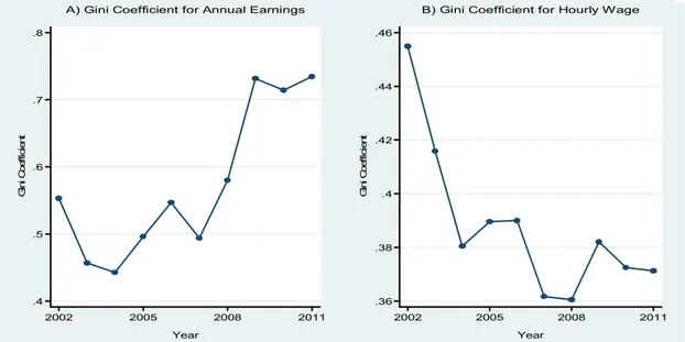
The measure of inequality is the Gini coefficient. From 2002 to 2007 the Gini coefficient for annual earnings is relatively constant, in the 0.45 to 0.55 band, but after 2007 it increases rapidly. From 2009 to 2011, it is above 0.7. The Gini coefficient for the hourly wage rate has a decreasing trend, especially during the 2002-2004 period. This might be the effect of the major economic crisis in 2001.
14
Figure 1 Gini Coefficients for Annual Earnings and Hourly Wage Rate, 2002-2011
These opposite trends are explained with increases in the variance of log annual hours and the covariance between log annual hours and log hourly wage rate increases during that period.
The following relationship is defined for these variables:
log (annual earnings) = log (hourly wage rate) + log (annual hours of work) Thus, taking into account the variance of both sides:
Variance of log annual earnings = Variance of log hourly wage + Variance of log annual hours + 2 * Covariance between log hourly wage and log annual hours
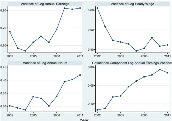
Figure 2 shows the variance of log annual earnings and its components. The variance of log annual earnings changes over time, and is very similar to the change in the Gini coefficient for log annual earnings given in Figure 1. Similarly, the change in the variance of log hourly wage rate over time in Figure 2 is very similar to the change in the Gini coefficient for log hourly wage rate in Figure 1.
.4 .5 .6 .7 .8 G in i C oe ffi ci ent 2002 2005 2008 2011 Year
A) Gini Coefficient for Annual Earnings
.36 .38 .4 .42 .44 .46 G in i C oe ffi ci ent 2002 2005 2008 2011 Year
15
Figure 2 illustrates the differences between the inequality measures of annual earnings and hourly wage rate. The decline in inequality between 2002 and 2004 (after the economic crisis) for annual earnings is not as pronounced as the decline in inequality for the hourly wage rate because the covariance component of the log annual earnings variance increases during this period. In addition, the rise in earnings inequality after 2007 is much higher than the rise in hourly wage inequality because both the variance of log annual hours and the covariance between log annual hours and log hourly wage rate increase during this period.
Figure 2 Log Annual Earnings Variance and its Components, 2002-2011 0.60 0.70 0.80 0.40 0.50 0.60 0.30 0.35 0.40 0.45 -0.10 -0.05 0.00 2002 2005 2008 2011 2002 2005 2008 2011 2002 2005 2008 2011 2002 2005 2008 2011
Variance of Log Annual Earnings Variance of Log Hourly Wage
Variance of Log Annual Hours Covariance Component Log Annual Earnings Variance
16
2.2. EARNINGS INEQUALITY ANALYSIS BY PERCENTILE GROUPS
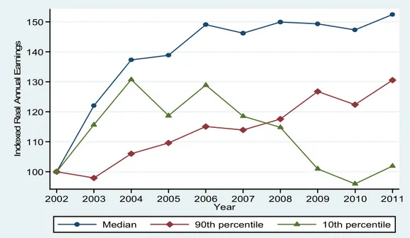
For a deeper look at earnings inequality, we examine the changes in real annual earnings for the period between 2002 and 2011 at three percentiles: median, the 90th percentile, and the 10th percentile. Each is normalized to 100 in 2002.
For the whole period, we can see a steady growth in the 90th percentile of the earnings distribution from 2002 to 2011, which totals about 30 percent. From 2002 to 2004, the median and 10th percentile show a clear increase, which can be interpreted as a recovery period right after the economic crisis.
The median and 10th percentile distributions start to show differences after 2006. After 2006, the median real annual earnings stay relatively constant at a level that is about 50% higher than that in 2002. On the other hand, there is a remarkable decline in the real annual earnings of the 10th percentile; even in 2010 the level of real annual earnings of the 10th percentile is below that of 2002. If we consider the picture as a whole for the percentile groups, we can say that there are different trends for the change in annual earnings, especially between 2006 and 2011, which points to increase in inequality as we saw in Figure 1.
17
Figure 3 Indexed Real Annual Earnings by Percentile, 2002-2011
2.3. EARNINGS INEQUALITY BY AGE
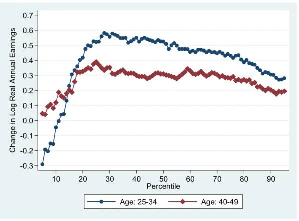
In this section, we compare the 25 to 34-year-olds (referred to as the younger group) to the 40 to 49-year-olds (referred to as the older group). Generally, the change in real annual earnings is higher for the younger age group. We know that the earnings of younger individuals are lower than those of older individuals in 2002; this leads us to believe that the inequality between age groups declines from 2002 to 2011 at most percentiles. This might be the effect of the growth of a more qualified and better educated workforce (assuming the younger generation is generally educated) in recent years and also an institutional change movement which outstands the young, dynamic workforce in corporate companies.
Since the trends of these two age groups generally have the same tendencies, it is useful to examine the within-age-group inequality. The 90th percentile to 50th percentile earnings difference declines for both age groups.
100 110 120 130 140 150 In de xe d R ea l A nn ua l E a rn in g s 2002 2003 2004 2005 2006 2007 2008 2009 2010 2011 Year
18
Moreover, the difference between these differences across age groups decreases because the decline in the 90th to 50th earnings gap is higher for the younger age group. The 50th percentile to 10th percentile earnings difference widens for both age
groups. Since it widens more for the younger group, the difference between the groups in the 50th to 10th percentiles earnings gap also widens. Overall, these findings indicate that increases in within-age-group earning inequalities are responsible for the increase in aggregate earnings inequality.
Figure 4 Log Real Annual-Earnings Changes by Percentile for Selected Age Groups
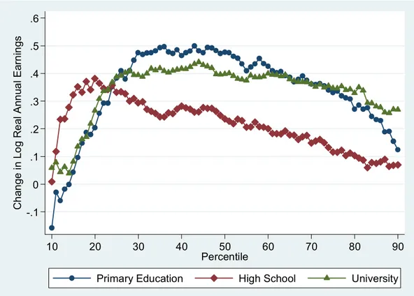
2.4.EARNINGS INEQUALITY BY EDUCATION LEVEL
In this section, we will examine the change in real annual earnings from 2002 to 2011 by education. The profiles of annual earnings changes by percentile are very similar for college graduates and primary school graduates. The earnings gap between college graduate and high school graduates increases between 2002 and
-0.3 -0.2 -0.1 0.0 0.1 0.2 0.3 0.4 0.5 0.6 0.7 Ch an ge in Lo g R e al A nn ua l E ar n in gs 10 20 30 40 50 60 70 80 90 Percentile Age: 25-34 Age: 40-49
19
2011, whereas the earnings gap between high school graduates and primary school graduates decreases.
As a result, we can suggest an increase in earning inequality for more skilled workers. When we examine within-group inequality by education, there is no clear tendency for high school and primary school graduates. On the other hand, we see that the within-group inequality for college graduates increases because while the percentage change in annual earnings for all percentiles above the 30th percentile is similar, that for percentiles below the 30th percentile is markedly lower.
Institutional changes and technological changes in the labor market might affect the unskilled, less educated individuals and therefore lower percentiles tend to decrease while upper percentiles tend to increase.
Figure 5 Log Real Annual-Earnings Changes by Percentile for Education Groups, 2002-2011 -.1 0 .1 .2 .3 .4 .5 .6 Ch an ge in Lo g R e al A nn ua l E ar n in gs 10 20 30 40 50 60 70 80 90 Percentile
20
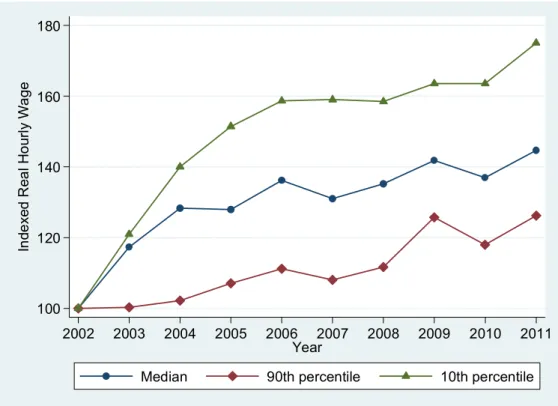
2.5. WAGE INEQUALITY ANALYSIS BY PERCENTILE GROUPS
In this section, we examine wage inequality by using percentiles of indexed real hourly wage from 2002 to 2011. After normalizing the 2002 value to 100, we observe that the median, 90th percentile, and 10th percentile all have the same tendency to increase.
The difference between the 90th and 10th percentiles’ increase shows the decline of inequality, which is also shown in Figure 1.
The comparison of real hourly wage and annual earnings graphics brings out the different behavior of the 10th percentile. This is because the 90th percentile and median increase in both graphics. However, the 10th percentile experiences an increase in real hourly wage together with a decrease in annual earnings. Hence, this divergence might explain Figure 1, which shows that the Gini coefficient for annual earnings increases whereas the Gini coefficient for real hourly wage decreases.
Figure 6 Indexed Real Hourly Wage Rate by Percentile, 2002-2011
100 120 140 160 180 In de xe d Re al H ou rl y W a ge 2002 2003 2004 2005 2006 2007 2008 2009 2010 2011 Year
21
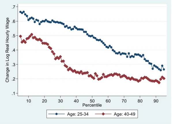
2.6. WAGE INEQUALITY BY AGE
In this section, we will compare the 25 to 34-year-olds (referred to as the younger group) with the 40 to 49-year-olds (referred to as the older group).
The older group has a lower increase in log real hourly wages compared to the younger group. The higher change of the younger group at most percentiles has a narrowing effect on wage inequality.
When we examine within-group inequality, we can say that inequality declines from 2002 to 2011 for both age groups since the log hourly wage rate is always higher for the lower percentiles.
Figure 7 Log Real Hourly Wage Changes by Percentile for Selected Age
Groups, 2002-2011 .1 .2 .3 .4 .5 .6 .7 Ch an ge in Lo g Re al H o ur ly W ag e 10 20 30 40 50 60 70 80 90 Percentile Age: 25-34 Age: 40-49
22
2.7. WAGE INEQUALITY BY EDUCATION LEVEL
In this section, we will examine the change in real hourly wage from 2002 to 2011 by education level. Since the log hourly wage rate is always higher for primary school graduates then high school graduates, it can be said that the wage inequality between high school and primary school graduates decreases from 2002 to 2011.
If we examine the within-group inequality, the same profile of primary and high school graduates shows us that the change at the lower percentiles is higher than the other percentiles, therefore within-group inequality in the hourly wage rate declines both for primary school graduates and high school graduates. Conversely, for the college graduates, the change at the lower percentiles is lower than the other percentiles and the change at most percentiles appears to be steady, thus there is no clear evidence of change in the within-group inequality.
Figure 8 Log Real Hourly Wage Changes by Percentile for Education Groups, 2002-2011 0 .1 .2 .3 .4 .5 .6 C h an ge in Lo g Re al H o ur ly W ag e 10 20 30 40 50 60 70 80 90 Percentile
23
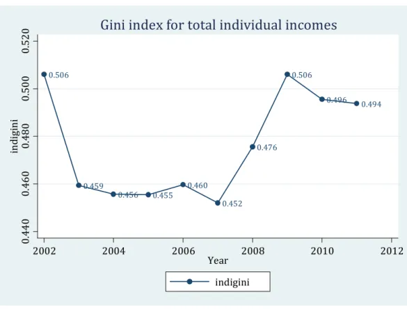
2.8. INCOME INEQUALITY
Income inequality includes asset income, labor income and household income. In the following analysis, we will only use individuals who are older than 15.
Firstly, a Gini index is calculated for total individual income from 2002 to 2011.The recovery from the 2001 crisis can be seen as a decline of the Gini coefficient until 2007. After 2007 the Gini index increases rapidly, as we see in Figure 1.
Figure 9 Gini Index for Total Individual Income
After the individual income analysis, we will make a similar examination in household income from 2002 to 2011. The overall trends have similarities to
0.506 0.459 0.456 0.455 0.460 0.452 0.476 0.506 0.496 0.494 0. 44 0 0. 46 0 0. 48 0 0. 50 0 0. 52 0 in di gi ni 2002 2004 2006 2008 2010 2012 Year indigini
24
individual income. The Gini index falls from 2002 to 2003 but the household income Gini has a more rapid decline after 2003. After 2007, the same increase starts with a lower rise when compared to individual income.
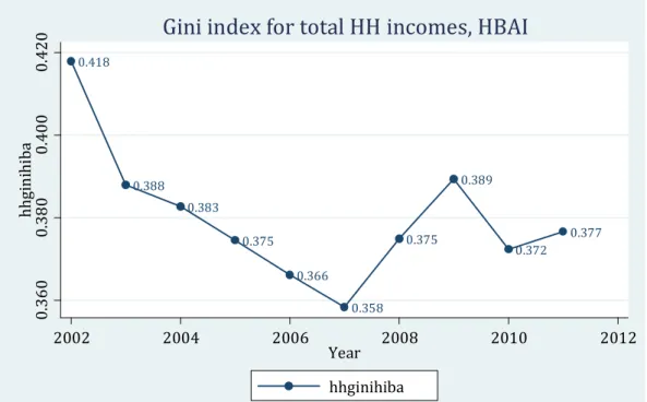
Figure 10 Gini Index for Total Household Income
2.9. INCOME INEQUALITY ANALYSIS BY PERCENTILE GROUPS
The median, 90th percentile, and 10th percentile individual total income from 2002 to 2011 are shown in Figure 11. Until 2006, there is a steady growth for all percentiles. But in 2009, there is a significant decrease, especially for the median, yet the median indiviudal income recovers in 2011 to its 2006 level. If we consider the whole period, the total changes of the median and 90th percentile are bigger than the 10th percentile’s change. 0.418 0.388 0.383 0.375 0.366 0.358 0.375 0.389 0.372 0.377 0. 36 0 0. 38 0 0. 40 0 0. 42 0 hh gin ih ib a 2002 2004 2006 2008 2010 2012 Year hhginihiba
Notes: Households' incomes are corrected for the household size according to the HBAI coefficient. This correction requires the information for the composition of the household
which is taken from the Turkish Statistical Institute data
25
The difference between the changes in individuals’ total incomes and annual earnings can be seen by comparing Figure 11 and Figure 3. While the 10th percentile has a decline after 2007 in Figure 3, we see an increase in Figure 11 for the same period. Median value has a steady growth of almost 50% of the levels in Figure 3, and in Figure 11, even though it shows a total growth of almost 50% between 2006 and 2009, there is a sharp decline in the index.
These differences can be explained by the effect of non-earnings income since the total income consists of earnings and non-earnings income. Later, in the distribution and decomposition sections, we will explain these two income sources seperately.
Figure 11 Median, 90th Percentile, and 10th Percentile Individual Income, 2002-2011
100 110 120 130 140 In de xe d In di vi du al Inco m e 2002 2003 2004 2005 2006 2007 2008 2009 2010 2011 Year
26
In Figure 12, we observe the percentiles of real household income from 2002 to 2011. We see a steady growth for all percentiles, where the minimum growth is 25% and the maximum growth is nearly 40%. Since the 10th and 50th percentiles had
a bigger growth than the 90th percentile, we can say that the difference between these percentiles decreases household income inequality. The lower Gini coefficient can be also seen in Figure 10.
Figure 12 Median, 90th Percentile, and 10th Percentile Household Income, 2002-2011
100 110 120 130 140 In de xe d R ea l H o us e hol d In co m e 2002 2003 2004 2005 2006 2007 2008 2009 2010 2011 Year
27
2.10. INCOME INEQUALITY BY EDUCATION LEVEL
Individual total income percentiles from 2002 to 2011 are analized by education level and indexed income values are shown in Figure 13. For all education levels, there is a steady growth in the median, while the 10th percentile has a fluctuating change.
Furthermore, there is no significant change in the 90th percentile, especially for primary school and high school graduates. For the primary school group, there is a remarkable decline after the year 2007, which brings the income under the value of that of 2002.
From 2002 to 2011, the minimum total growth of the median and 90th percentile is almost 10% and the maximum is nearly 40% across the education groups, which can be interpreted as an important growth in income. The 10th
percentile income has a deep decline for primary school graduates while high school and college graduates have a relatively lower decline.
28
Figure 13 Median, 90th Percentile, and 10th Percentile Individual Income by Education Level, 2002-2011
2.11. INCOME INEQUALITY BY WORK EXPERIENCE
In Figure 14, the median, 90th percentile, and 10th percentile individual total incomes are shown from 2002 to 2011 for both less experienced and more experienced groups. For both experience groups, there is an important growth in the median and 90th percentile for the long term. On the other hand, the 10th percentile differs for experience groups; the less experienced group has a volatile but steady growth while the more experienced group first experiences an increase then a slow, steady decline. 60 80 10 012 014 0 In de xe d re al inc om e 2002 2004 2006 2008 2010 2012 year 10th percentile median 90th percentile
primary school graduates
80 10 012 014 016 0 In de xe d re al inc om e 2002 2004 2006 2008 2010 2012 year 10th percentile median 90th percentile
high school graduates
80 10 0 12 0 14 0 In de xe d re al inc om e 2002 2004 2006 2008 2010 2012 year 10th percentile median 90th percentile college graduates
29
If we consider the whole period, the total growth of the 90th percentile is 45% or more and the total growth of the 10th and 50th percentiles are around 20% for the less experienced group. But for the more experienced group, this amount of growth can not be seen for any percentiles. The 90th percentile’s and median’s growth are around 20% and the 10th percentile has a deep decline, around 40%.
Figure 14 Median, 90th Percentile, and 10th Percentile Individual Income by Work Experience Groups, 2002-2011
10 0 12 0 14 0 16 0 In de xe d re al inc om e 2002 2004 2006 2008 2010 2012 year 10th percentile median 90th percentile less experienced 60 80 10 0 12 0 14 0 16 0 In de xe d re al inc om e 2002 2004 2006 2008 2010 2012 year 10th percentile median 90th percentile more experienced
30
2.12. INCOME INEQUALITY BY AGE GROUPS
In Figure 15, the median, 90th percentile and 10th percentile individual total incomes are shown from 2002 to 2011 for both younger and older groups. For the younger group, there is a clear growth in the median and 90th percentile for the long term. On the other hand, the 10th percentile has an up and down trend which ends with a deep decline.
For the older age group, the median shows growth until 2005 and then real income starts to decrease, the 90th percentile seems to have a fluctuating trend without a significant change in the total, and the 10th percentile first shows major growth from 2002 to 2003 and then it starts to decrease rapidly.
Considering the whole period, the median and the 90th percentile have significant growth for both age groups, but the younger group’s growth is relatively higher, around 20%. Furthermore, the 10th percentile’s decrease is around 40-50% for both age groups.
31
Figure 15 Median, 90th Percentile, and 10th Percentile Individual Income by Age Groups, 2002-2011
2.13. INCOME DISTRIBUTION, 2002-2011
The following figure illustrates the distribution of income sources consisting of earnings, non-earnings and total income separately in the following years: 2002, 2005, 2008, and 2011. The figure shows that the earnings income and non-earnings income both affect total income.
There is not a clear change for earnings, non-earnings, or total income over the years. Only the distribution of non-earnings has a higher density than the distribution of earnings density at some levels of income between 0-6 logarithmically. Afterwards, the distribution of non-earnings’ density starts to coincide with the earnings and total income.
60 80 10 0 12 0 14 0 In de xe d re al in come 2002 2004 2006 2008 2010 2012 year 10th percentile median 90th percentile Age group 25-34 60 80 10 0 12 0 14 0 In de xe d re al in come 2002 2004 2006 2008 2010 2012 year 10th percentile median 90th percentile Age group 40-49
32
At the level of the individuals’ income between 7-9 (log), the density of the distribution of earnings is always higher than the distribution of non- earnings income.
Figure 17 shows the distribution of income by illustrating the shares of earnings and non-earnings per household. Since the y-axis shows the income level, we see that non-earnings generally stay at a low level while the earnings are at higher levels. This figure also indicates that earnings income is the most important share of household income.
33
Figure 16 Earnings, Non-Earnings and Total Income Distributions, 2002-2005-2008-2011 0 .2 .4 .6 De ns ity 0 2 4 6 8 10 12 14 log(income) earnings nonearnings total
kernel = epanechnikov, bandwidth = 0.1310 2002 distributions 0 .2 .4 .6 De ns ity 0 2 4 6 8 10 12 14 log(income) earnings nonearnings total
kernel = epanechnikov, bandwidth = 0.1280 2005 distributions 0 .2 .4 .6 De ns ity 0 2 4 6 8 10 12 14 log(income) earnings nonearnings total
kernel = epanechnikov, bandwidth = 0.1477 2008 distributions 0 .2 .4 .6 De ns ity 0 2 4 6 8 10 12 14 log(income) earnings nonearnings total
kernel = epanechnikov, bandwidth = 0.1502 2011 distributions
34
Figure 17 Earnings and Non-Earnings Income Distribution of Households, 2002 - 2005 - 2008 - 2011 0 50 00 0 10 00 00 15 00 00 in co m e 200000 202000 204000 206000 208000 210000 household earnings nonearnings 0 50 00 0 10 00 00 15 00 00 in co m e 500000 502000 504000 506000 508000 household earnings nonearnings 0 50 00 0 10 00 00 15 00 00 20 00 00 in co m e 800000 802000 804000 806000 808000 household earnings nonearnings 0 50 00 0 10 00 00 15 00 00 20 00 00 in co m e
1.1e+06 1.1e+06 1.1e+06 1.1e+06 household
35
2.14. DECOMPOSITION OF INCOME INEQUALITY
To examine the earnings and non-earnings income and their effect on the total income inequality, a decomposition is made by using the methodology of Stark, Taylor and Yitzhaki. This decomposition is shown in Table 1.
The first column is the proportion of earnings and non-earnings income to total income (Sk), the second column is the Gini indices calculated when earnings and non-earnings are used separately (Gk), the next column is the correlation of earnings and non-earnings with the distribution of total income (Rk), and the following column is the share of each income source in total inequality (share). In the last column Gini is calculated excluding the zero income variables, which hashas a decreasing effect on the Gini index.
The share of earnings in the total individual income data is always at 70%; this indicates that earnings income is the most important share of the individual data. The Gini index calculated for non-earnings is relatively higher than the Gini index calculated for earnings income. This indicates that the distribution of the non-earnings income is more dispersed than the non-earnings distribution. Another point about the change on gini index values is that the both indexes decrease until the year 2007, but after 2007 both of them increase. This is also seen in Figure 9. The next column and the correlation show that earnings are more correlated with total income; this is also consistent with the share values since the proportion of earnings in the total income of individuals is much higher than that of non-earnings income. The share column shows that the proportion of earnings in total individual income inequality is between 75% and 80%. In the last column, the Gini index values are calculated by eliminating the individuals with zero earnings and non-earnings; this
36
elimination reduced the Gini index values since the Gk column is lower than the Gini column for all years.
Table 1 Decomposition of Income Inequality
Sk Gk Rk Share Gini 2002 Earnings 0.738 0.632 0.867 0.805 0.512 Nonearnings 0.262 0.764 0.489 0.195 0.641 2003 Earnings 0.735 0.613 0.837 0.817 0.476 Nonearnings 0.265 0.756 0.421 0.183 0.563 2004 Earnings 0.733 0.623 0.845 0.822 0.477 Nonearnings 0.267 0.737 0.423 0.178 0.579 2005 Earnings 0.714 0.619 0.840 0.784 0.473 Nonearnings 0.286 0.725 0.493 0.216 0.585 2006 Earnings 0.721 0.625 0.855 0.795 0.472 Nonearnings 0.279 0.735 0.483 0.205 0.607 2007 Earnings 0.722 0.644 0.853 0.806 0.472 Nonearnings 0.278 0.746 0.460 0.194 0.621 2008 Earnings 0.705 0.654 0.845 0.795 0.501 Nonearnings 0.295 0.739 0.461 0.205 0.582 2009 Earnings 0.707 0.649 0.857 0.777 0.518 Nonearnings 0.293 0.758 0.510 0.223 0.556 2010 Earnings 0.700 0.647 0.850 0.779 0.505 Nonearnings 0.300 0.747 0.490 0.221 0.537 2011 Earnings 0.719 0.640 0.856 0.797 0.508 Nonearnings 0.281 0.757 0.472 0.203 0.532
37
2.15. RESULTS
First of all, it is observed that the inequality between the age groups declines from 2002 to 2011 at most percentiles and the earnings gap between college graduate and high-school graduates increases between 2002 and 2011, whereas the earnings gap between high-school graduates and primary school graduates decreases. Next, we saw in particular the different behavior of the Gini indices of annual earnings and hourly wage. An analysis of income inequality in Turkey shows that for individuals, the Gini coefficient as well as the household income Gini decreases until the year 2007, possibly as an effect of the recovery from the 2001 crisis.
These distribution figures did not reveal a clear change for earnings and total income over the years.
The decomposition at the end of this chapter demonstrated that earnings income is the most important share of the individual data and the distribution of the non-earnings income is more spread out than the earnings distribution.
38
CHAPTER THREE
REGRESSION ANALYSIS OF INCOME INEQUALITY IN TURKEY, 2002-2011
3.1. COHORT INCOME INEQUALITIES: PANEL DATA STRUCTURE
In this section, the micro-income dataset is used to demonstrate within-cohort income inequalities. Since this dataset does not have a panel structure, we construct synthetic within-cohort inequality data using separate cross-sectional datasets. For example, the inequality index in 2002 is calculated for individuals aged 21-25 years. In 2003 the same index is calculated for individuals aged 22-26 years, whereas these are not necessarily the same individuals as in 2002.
The way we constructed the individuals’ ages is illustrated below:
Cohort 1 (16-20 in 2002) Cohort 2 (21-25 in 2002) Cohort 10 (61-65 in 2002)
2002 Individuals aged 16-20 Individuals aged 21-25 Individuals aged 61-65
2003 Individuals aged 17-21 Individuals aged 22-26 Individuals aged 62-66
...
39
3.2. ANALYSIS BY GINI INDEX
Figure 18 shows the within-group inequalities that follow the 2002-2011 period. We see that the within-cohort inequalities tend to decrease from 2002 to 2004, and then they start to increase again, which is consistent with the aggregate Gini index that was calculated for individuals in the second chapter. But other than this period, we expect increases in within-cohort inequalities in younger cohorts but decreases in within-cohort inequalities in older cohorts. This is because individuals’ earnings change through their lifetimes, so this causes a more dispersed income distribution for young cohorts. As people retire, their incomes get closer to one other. Since the expected increase did not happen for the 2002-2004 period, this might be the effect of the recovery period after the 2001 crisis.
40
Figure 18 Gini Indexes Calculated for Cohorts
.3 .3 5 .4 .4 5 G ini Index 2002 2004 2006 2008 2010 2012 Year Cohorts of Aged 16-20 in 2002 .3 .3 5 .4 .4 5 G ini Index 2002 2004 2006 2008 2010 2012 Year Cohorts of Aged 21-25 in 2002 .3 .3 5 .4 .4 5 G ini In dex 2002 2004 2006 2008 2010 2012 Year Cohorts of Aged 26-30 in 2002 .3 .3 5 .4 .4 5 G ini In dex 2002 2004 2006 2008 2010 2012 Year Cohorts of Aged 31-35 in 2002 .3 .3 5 .4 .4 5 G ini Ind ex 2002 2004 2006 2008 2010 2012 Year Cohorts of Aged 36-40 in 2002 .3 .3 5 .4 .4 5 G ini Ind ex 2002 2004 2006 2008 2010 2012 Year Cohorts of Aged 41-45 in 2002 .3 .3 5 .4 .4 5 G in i I nde x 2002 2004 2006 2008 2010 2012 Year Cohorts of Aged 46-50 in 2002 .3 .3 5 .4 .4 5 G in i I nde x 2002 2004 2006 2008 2010 2012 Year Cohorts of Aged 51-55 in 2002 .3 .3 5 .4 .4 5 G ini In dex 2002 2004 2006 2008 2010 2012 Year Cohorts of Aged 56-60 in 2002 .3 .3 5 .4 .4 5 G ini In dex 2002 2004 2006 2008 2010 2012 Year Cohorts of Aged 61-65 in 2002
41
3.3. COMPARISON OF MEASURES OF INEQUALITY
The results of comparing average growth in within-cohort inequality to growth in the aggregate (average within-cohort) inequality are in Figure 19. Three measures of inequality are considered: the average growth rate of within-cohort inequalities for the heads of households aged 16-65, the growth rate of aggregate inequality calculated for the heads of households aged 16-65, and the growth rate of aggregate inequality, using the full sample of households.
The aggregate inequalities calculated using a full sample and the individuals aged 16-65 are very close and there is no significant difference between the average growth of within-cohort inequality and the growth of aggregate inequality.
The cohort inequality is also similar to the aggregate inequalities up until 2008. For 2009 and 2010, there is a significant variance between aggregate and cohort inequalities. As we have calculated the average of within-cohort inequalities, the decline in cohort inequality must be the effect of the lack of samples aged 68-72 in 2009 and those aged 69-73 in 2010. Finally, for the year 2011, cohort inequality once again reaches the level of aggregate inequality.
42
Figure 19 Average Growth in Within-Cohort Inequality vs. Growth in Aggregate (Average Within-Cohort) Inequality
3.4. EXPLANATION OF THE INCOME INEQUALITY IN TURKEY THROUGH REGRESSION ANALYSIS: EMPIRICAL FRAMEWORK
In this section, two different regression models will be used to explain income inequality in Turkey. In the previous chapter, we focused on three main inequality subjects: earnings, wage, and total income inequality. Firstly, an estimation model will be constructed with the available explanatory variables for these inequality subjects.
Since the earnings income mostly consist of employed individuals’ income, we have focused on the individuals whose labor force attachment is stronger; through these calculations, some variables that may affect the labor force are obtained.
-1 .0 5 -1 -. 9 5 -. 9 -. 8 5 -. 8 Gi ni Ind ex G ro wt h 2002 2004 2006 2008 2010 2012 Year Cohort AggregateCohort AggregateFull
Cohort: Average growth in within-cohort inequality (unweighted) Aggregate, Full Sample: Growth in aggregate inequality Aggregate Cohort Sample: Growth in aggregate inequality
the latter is calculated with the households of aged between 16 and 65
43
In Chapter Two, we have analyzed all three subjects by education level groups and we have observed that an increase in the education level may also cause an increase in inequality; therefore the variables of education and the labor force with at least a secondary education are used in the model.
Since one part of Chapter Two consists of wage inequalities, waged workers’ shares will be placed in the model.
The decomposition of income inequality showed us that non-earnings income has a higher density at lower percentiles. This may be the result of the social benefits provided by the government to low-income individuals; therefore some social development indicators are generally reviewed but for Turkey, no such indicators could be found for the 2002-2011 period. To overcome this problem of the lack of data on social aid, we assumed that the government’s health expenditures can be taken as a substitute indicator for the government’s social benefits, and health expenditures will be placed in the model. Lastly, an inequality analysis by percentile groups which was also examined in the second chapter led us to add variables, which may explain the effect of some percentile groups’ shares in total income. The model is explained below:
ln = + ℎ + ln + ln ℎ
+ ℎ + + ℎ +
POPSHARE is the percentage of the population aged 15 and older with a secondary or higher education, and H is the average years of education in the population aged 15 and older. Health is the health expenditures provided by
44
government. Incshare is the total income share of the 90th percentile. Laborforce is the labor force participation rate. Wagedshare is the waged/salaried workers rate.
The second estimation model is taken from Chapter 4 of the IMF WEO (2007), which explains the change in the Gini coefficient across a sample of countries using a set of explanatory variables, focusing on trade. The model is explained below: 1 2 3 4 5 6 7 8 9 10 11 ln( ) ln( ) ln(100 ) ln( ) ln( ) ln( ) ln( ) ln( ) ln( ) , ICT AGR IND X M A L Gini α α α Tariff α Y Y K Credit α Kaopen α α α Popshare K Y E E α H α α ε E E
X and M are (non-oil) exports and imports, Y is the nominal GDP, and TARIFF is the average tariff rate. In the model (X+M)/Y is the de facto measure of trade globalization and (100-Tariff) is the de jure measure of trade globalization. These measures are used to assess the effect of trade liberalization on income inequality. The model also searches for the effect on inequality of financial liberalization by using the variables (A+L)/Y, where A and L represent cross-border financial assets and liabilities, and KAOPEN, the capital account openness index. KICT is the ratio of information communication technology capital stock to the total capital stock. This is an indicator of technological development, which is expected to increase income inequality by raising demand for skilled labor, but the Turkey data for this variable could not be found and will not be a part of this study. CREDIT is the volume of credit offered by deposit banks and other financial institutions to the private sector, and it shows the development of the financial sector in the economy. POPSHARE is the percentage of the population aged 15 and older with a secondary
45
or higher education, and H is the average years of education in the population aged 15 and older. Greater access to education is expected to reduce income inequality by enabling more people to access high-skill work activities. E is total employment, and EAGR and EIND are employment in agriculture and industry, respectively. These are used to calculate sectoral percentages of employment, which is important because the move from agriculture to industry is expected to reduce inequality by reducing the number of low-earning income groups.
3.5. VARIABLES USED IN THE REGRESSION MODELS: EDUCATION
The average years of schooling in the population aged 15 and older, and the number of the population aged 15 and older with secondary and/or higher education variables are used in the model. The data are collected from Barro-Lee’s (2000) dataset. Since the data is available only for the years 2005 and 2010, the other years’ values are calculated using interpolation/extrapolation methods.
3.6. SOCIAL DEVELOPMENT/ HEALTH EXPENDITURE
Data on health expenditures provided by government have been collected from the World Bank.
3.7. INCOME DISTRIBUTION
The total income share of the 90th percentile is in the total share and is used to analyze the effect of change in the income shares. This data is collected from The World Bank. The labor force participation rate and waged/salaried workers share in the total employment are also collected from The World Bank. For 2011, some of