Quasi-two-dimensional Feynman bipolarons

Quasi-two-dimensional Feynman bipolarons

R. T. Senger and A. Erc¸elebi

Department of Physics, Bilkent University, 06533 Ankara, Turkey

共Received 15 January 1999兲

We study the stability criterion for the formation of two-dimensionally confined large bipolarons. The electrons are treated as bounded within a parabolic potential well while being coupled to one another via the Fro¨hlich interaction Hamiltonian. Within the framework of the bulk-phonon approximation we adopt the Feynman-polaron model to derive variational results over a wide range of the Coulomb interaction and phonon coupling strengths interpolating between the bulk and the two-dimensional confinement limit. It is shown that the critical values of the electron-phonon coupling constant and the ratio of dielectric constants (␩⫽⑀_⬁/⑀0) exhibit some nontrivial features as the effective dimensionality is tuned from 3 to 2.关S0163-1829共99兲08637-3兴

I. INTRODUCTION

Two electrons in a polar or ionic crystal interact with the lattice vibrations resulting in attractive forces between them. Under certain conditions, the phonon mediated attraction be-tween the particles may come out to be strong enough to counterbalance the Coulomb repulsion and consequently, a stable bound state can form. Such a state of the system con-sisting of the pair of electrons and a common density of virtual phonons is termed a bipolaron.

Among the numerous amount of papers published within the context of two-polaron systems, we at first cite the pio-neering work of Haken1who studied the problem of the in-teraction between an electron and a hole via the coupling to the LO branch of the phonon spectrum in polar semiconduc-tors. Using a variational method he showed that the polaron corrections to the effective interaction at large distances de-crease exponentially, reflecting the exponentially decreasing overlap between the clouds of bound charges around the po-larons. The same problem was further considered by Mahanti and Varma2and by Sak3where they included the corrections to the electron-hole potential coming from the dynamic po-larization of the lattice, and showed how deviations from the Coulomb form could occur. The intrinsic effect of electron

共hole兲 phonon interactions on the nature of forces acting

be-tween the particles was reconsidered by Kuleshov, Matveev, and Smondyrev4and the same work was revised later.5 Bas-ing their calculations on Feynman path-integral formalism, they developed a scheme for obtaining expressions for the particle interaction potentials and the ground state energy in both the strong- and weak-coupling approximations. A simi-lar problem in the same area was considered by Bishop and Overhauser6 to investigate the phonon-mediated interaction between two electrons where they showed that for ionic crys-tals the effective electron-electron potential may lead to an attractive deep potential well with a minimum occurring for particle separations as small as a few tens of Å.

In the bipolaron problem, with the electrons being closely positioned, the polarization fields centered about the particles overlap and interfere in a constructive manner to create a potential well deep enough to compete with the Coulomb repulsion so as to prevent the particles from being projected apart. Depending on the dielectric properties of the medium,

provided the effective Coulomb repulsion is not larger than a critical strength and the phonon coupling constant is not smaller than a critical value, the lattice effects may account for a considerable part of the energy of the electron-electron pair which consists of attracting the particles against their Coulomb repulsion. Thus, the fundamental condition under which a bipolaron can exist is that the repulsive Coulomb interaction should not be too strong to dominate over and hence break up the phonon-mediated binding which holds the particles together.

In the last two decades, the study of bipolarons has at-tracted a revived and extensive interest in the literature.7–26 Of particular relevance to the content of the present article are the recent solutions of the bipolaron problem in three and strict two dimensions14–16,21where it is observed that a bi-polaronic bound state of two electrons is more easily attained in two dimensions than in three. The concern of the present study is to extend the problem to a broader discourse and explore the stability of quasi-two-dimensional bipolarons confined in a parabolic quantum well with variable well width and potential barrier slopes; thus provide an interpo-lating insight into the phase diagram, encompassing the bulk and the two-dimensional limits. The harmonic-oscillator con-fining potential that we adopt here has already been used in a parallel study26 within the framework of the strong-coupling polaron theory where it has been noted that, in the quasi-two-dimensional 共slablike兲 configuration, the utmost permissible Coulomb strength which would allow a bipolaron state to form may turn out to be lower than one would have for the three- and strict two-dimensional bipolarons. To see whether this peculiar feature is indeed a characteristic of quasi-two-dimensionally confined bipolarons, we wish to review the problem within a similar framework of the three and two-dimensional bipolaron models set up earlier by Verbist, Peeters, and Devreese14where they reformulate the Feynman path-integral variational approach27to tackle the case of two interacting polarons. Thus, a critical understanding of the foregoing calculations and the outcomes depends heavily on having read Ref. 14 with which we shall make some frequent correspondence, particularly when the three- and two-dimensional limits of our model are concerned. We believe, the methodology followed in this work proves to be a pow-erful technique intended to yield a satisfactory description of

PRB 60

the problem in the overall ranges of the parameters charac-terizing the system. In the following, we obtain an explicit tracking of the phase stability in terms of the Coulomb and phonon-coupling strengths as a function of the effective di-mensionality tuned from 3 to 2.

II. THEORY A. Bipolaron model

The model that we use consists of a pair of quasi-two-dimensional electrons coupled to the LO branch of the bulk phonon spectrum. As such, the fundamental approach fol-lowed in this work is to account for mainly the generic low-dimensional aspect of the dynamical behavior of the elec-trons and visualize them as interacting with the medium and with one another through exhange of virtual phonons. Apart from ignoring the contributions that may come from all other kinds of phonon modes, we also omit the screening effects and further details, such as those due to the nonparabolicity corrections to the electron band or the loss of validity of both the effective-mass approximation and the Fro¨hlich con-tinuum Hamiltonian in microstructures. Hence, under the so-called bulk-phonon approximation and the aforementioned simplifying assumptions, we write the Hamiltonian describ-ing the confined electron-pair system coupled to the LO pho-non field as H⫽He⫹

兺

Q a_Q†aQ⫹

兺

i_⫽1,2

兺

Q VQ共aQeiQជ •rជi⫹aQ † e⫺iQជ•rជi兲, 共1兲 where He⫽

兺

i⫽1,2

冉

1 2pi 2_⫹V conf共zi兲

冊

⫹ U 兩rជ1⫺rជ2兩 . 共2兲

Here and henceforth we use dimensionless units appropriate to a polaron calculation and take m*⫽ប⫽␻LO⫽1. In Eqs.

共1兲, 共2兲, aQand aQ †

denote the phonon annihilation and cre-ation operators, and rជi⫽(␳ជi,zi) (i⫽1,2), are the positions of the electrons in cylindrical coordinates. Similarly, pជi (i

⫽1,2) denote the respective momenta of the electrons. The

Fro¨hlich interaction amplitude is related to the phonon wave vector Qជ⫽(qជ,qz) through

VQ⫽共2

冑

2␲␣兲1/2兩Qជ兩⫺1,

where ␣ is the coupling constant defined, in terms of the high frequency and static dielectric constants of the medium, by ␣⫽ e 2

冑

2

冉

1 ⑀⬁⫺ 1 ⑀0

冊

. 共3兲

In the Coulomb term, the unscreened amplitude U is related to the ratio of the dielectric constants

␩⫽⑀_⑀⬁ 0 ⬍1, 共4兲 through U⫽e 2 ⑀⬁⫽

冑

2 1⫺␩ ␣. 共5兲

For the confining potential we use a harmonic oscillator pro-file with adjustable barrier slopes, i.e., we set

Vconf共z兲⫽ 1 2⍀

2_z2 _共6兲

in which the dimensionless frequency⍀ serves for the mea-sure of the degree of confinement of the electron which, when tuned from zero to infinity, yields a unifying display of the phase stability of the bipolaron as a function of the ef-fective dimensionality ranging from 3 to 2. The rationale behind imposing quadratic potential profiles is that such a form for the confining barriers greatly facilitates the calcula-tions and leads to tractable analytic expressions. We have thus refrained ourselves from treating potentials of other forms which possibly would lead to complicated and even prohibitively difficult expressions and numerical complica-tions and yet yield qualitative features similar to those for parabolic potential shapes. Indeed, calculations pertaining to the cyclotron study of polarons confined to an interface in-dicate that the phonon-coupling-induced shift in the resonant energy is sensitive dominantly to the strength of the confin-ing potential rather than its shape.28 Moreover, due to the absence of an abrupt variation in the medium structure and properties, the parabolic confining potential allows us to dis-regard any relevance to the interface phonon modes.29 We, therefore, conveniently use the harmonic-oscillator potential

共6兲 as a simplifying first approximation compatible with the

framework of the path integral approach where one assumes the two electrons to be coupled to one another and to the corresponding fictitious particles via harmonic springs.

In the Feynman path integral representation of the po-laron, the phonon variables can be projected out exactly to yield the partition function of the bipolaron system in the form ZBP⫽ZphZ, 共7兲 where Zph⫽

兿

Q

冉

1 1⫺e⫺␤ប␻LO

冊

3 共8兲

is the phonon part, and

Z⫽

兿

i⫽1,2

冉

冕

drជ₀

冕

rជ_i(0)⫽rជ₀ rជ_i(␤)⫽rជ₀ Drជi共␭兲

冊

eS[rជ1(␭),rជ2(␭)] 共9兲 is the path integral in which the action S consists of two parts, one pertaining to the electron part of the Hamiltonian and the other to the electron-phonon interaction. In imagi-nary time variables (t→⫺i␭), we have respectively, the fol-lowing expressions: Se⫽⫺ 1 2

冕

0 ␤ d␭

兺

i⫽1,2关rជ ˙ i 2_{共␭兲⫹⍀}2_z i 2_{共␭兲兴⫹S} c, 共10兲 where

Sc⫽⫺

冕

0 ␤ d␭ U 兩rជ1共␭兲⫺rជ2共␭兲兩 共11兲

is the Coulomb term, and

Se- p⫽ 1 2 i_⫽1,2

兺

j

兺

_⫽1,2

兺

Q V_Q2

冕

0 ␤ d␭

冕

0 ␤ d␭

⬘

G(␻_LO⫽1)共␭⫺␭

⬘

兲 ⫻eiQជ •[rជ_i(␭)⫺rជ_j(␭⬘)] _共12兲 is the part describing the phonon mediated retarded attractive interaction between the electrons. In the above, the dimen-sionless parameter␤ stands for the inverse temperature, and the memory function

G_␻共u兲⫽cosh关共␤⫺2兩u兩兲␻/2兴

sinh共␤␻/2兲 共13兲 is the Green’s function of a harmonic oscillator with fre-quency ␻. In principle, at zero temperature, we have Z_BP

⫽Z, and the bipolaron ground state energy

E_g⫽⫺ lim ␤→⬁␤

⫺1_logZ,

can be calculated exactly provided the path integral 共9兲 can be evaluated. Since this is not possible due to the analytic complexity of the integral expressions in the action S, Eqs.

共10兲–共12兲, we choose to proceed with the introduction of a

solvable trial actionS0 intended to provide us with a conve-nient variational upper bound to the ground state energy, led by the Jensen-Feynman inequality

Eg⭐E0⫺ lim ␤→⬁

1

␤

具

S⫺S0

典

S₀, 共14兲

where the notation

具 典

_S

0 denotes a path-integral average

with density function eS0_{, and E}

0 is the trial ground state energy corresponding to S₀. The form of the trial action should be simple enough to permit analytical calculations and yet be detailed enough to cover all the basic features of the exact action S.

B. The trial model and its diagonalization

For the trial action we choose the model which was suc-cessfully applied to similar polaron or bipolaron problems14,27,30 where the electrons are considered to be in quadratic interaction with the fictitious masses. We writeS₀ as a sum of three terms, i.e.,

S0⫽Se⫹Ss⫹Sm, 共15兲 whereSeis similar to that given by Eq.共10兲, except now that the Coulomb term 共11兲 is reexpressed as

Sc⫽ 1 2K

冕

0

␤

d␭关rជ1共␭兲⫺rជ2共␭兲⫺aជ兴2. 共16兲

Ss and Sm refer to the self- and mutual interaction of the electrons with the fictitious masses, each with its own and with that of the other electron, respectively. These terms as-sume the following path-integral representations

Ss⫽⫺ cs 2

冕

0 ␤ d␭

冕

0 ␤ d␭

⬘

Gw共␭⫺␭

⬘

兲

兺

i⫽1,2关r ជi共␭兲⫺rជi共␭

⬘

兲兴2, 共17兲 Sm⫽⫺2⫻ c_m 2

冕

0 ␤ d␭

冕

0 ␤ d␭

⬘

Gw共␭⫺␭

⬘

兲 ⫻关rជ1共␭兲⫺rជ2共␭

⬘

兲⫺aជ兴2. 共18兲 In the above K, cs, cm and w are variational parameters introduced within a similar context as in the original paper by Feynman.27Vector aជ is a further parameter describing the mean distance between the central positions about which the electrons fluctuate. We should note that the confining poten-tial 共6兲, being symmetric in the ⫾z directions, imposes the mean positions of both electrons to lie in the x y plane. We therefore readily set az⫽0. We should also remark that in the extreme limits aជ⫽0 and 兩aជ兩→⬁, the model yields re-spectively a description of either the bipolaronic state of the two electrons or a pair of two independent polarons.14

Since the trial action and the path-integral averages in-volved in Eqs. 共14兲–共18兲 are all separable in the Cartesian coordinates, the calculations can be performed all in identical manners for each spatial direction. Denoting the Cartesian component of the ith electron in any chosen direction by xi and that of the ith fictitious mass M by Xi, the part of the model Lagrangian relevant to that coordinate

Lmod (x) _⫽1 2 i⫽1,2

兺

共x˙i 2_⫺⍀2_x i 2_⫹MX˙ i 2_兲⫹K 2共x1⫺x2⫺ax兲 2 ⫺␬₂

兺

i⫽1,2共xi⫺Xi兲 2 ⫺␬₂

⬘

兵共x1⫺X2⫺ax兲2⫹共x2⫺X1⫹ax兲2其 共19兲 can be related to the following model action:

Smod (x)_⫽⫺1 2

冕

0 ␤ d␭

兺

i⫽1,2关x˙i 2_{共␭兲⫹⍀}2_x i 2_{共␭兲⫹MX˙} i 2_共␭兲兴 ⫹1 2

冕

0 ␤ d␭

再

K关x1共␭兲⫺x2共␭兲⫺ax兴2 ⫺

兺

i_⫽1,2␬关xi共␭兲⫺Xi共␭兲兴 2

冎

⫺␬

⬘

2

冕

0 ␤ d␭兵关x1共␭兲⫺X2共␭兲⫺ax兴2 ⫹关x2共␭兲⫺X1共␭兲⫹ax兴2其. 共20兲 Here, it should be understood that⍀ has its original meaning as in Eq.共10兲 when one refers to the z direction, but assumes zero value for the remaining two directions.

Similar to the elimination of the phonon degrees of free-dom, also eliminating the fictitious mass coordinates Xi, we obtain the relevant trial action, expressed solely in terms of the electron coordinates, in the form as given in Eqs.共15兲–

共18兲. The variational parameters of the trial action can then

be identified in terms of the parameters of the model La-grangian w⫽

冑

␬⫹␬

⬘

M , cs⫽ ␬2_⫹␬

_⬘

2 4 M w , cm⫽ ␬␬

⬘

2 M w. 共21兲 In order to calculate the ground state energy of the varia-tional model and the path integral average required in Eq.

共14兲, one needs to diagonalize Lmod

(x) _{共19兲. Introducing} xc.m.(Xc.m.) and xrel(Xrel) as the center of mass and relative coordinates for the electrons共fictitious masses兲 through

再

x1 x2

冎

⫽1 2共xc.m.⫾xrel兲⫾ ax 2 ,

再

X1 X2

冎

⫽1 2共Xc.m.⫾Xrel兲⫾ ax 2

we rewrite the Lagrangian relevant to the chosen direction as

Lmod (x) _⫽L c.m. (x)_⫹L rel (x) , where L_c.m.(x)⫽1 4x˙c.m. 2 _⫹1 4M X˙c.m. 2 _⫺1 4共⍀ 2_⫹␬⫹␬

_⬘

_兲x c.m. 2 ⫺1 4共␬⫹␬

⬘

兲Xc.m. 2 _⫹1 2共␬⫹␬

⬘

兲xc.m.Xc.m., 共22兲 L_rel(x)⫽1 4x˙rel 2 _⫹1 4M X˙rel 2 _⫺1 4共⍀ 2_{⫹2K⫹␬⫹␬}

_⬘

_兲x rel 2 ⫺1 4共␬⫹␬

⬘

兲Xrel 2 _⫹1 4共␬⫺␬

⬘

兲xrelXrel. 共23兲 We should note that we have excluded a final term

⫺1 2⍀

2_a

xxrelwhich has had to appear on the right hand side of Eq. 共23兲, since this term always vanishes because, either

⍀ or ax is zero for all Cartesian directions. Under appropriate coordinate transformations

x_c.m.⫽␩₀⫹␩₁, Xc.m.⫽ w2 w2⫺␰₀2␩0⫹ w2 w2⫺␰₁2␩1, 共24兲 x_rel⫽␩₂⫹␩₃, Xrel⫽ ␬⫺␬

⬘

␬⫹␬

⬘

w2 w2⫺␰₂2␩2⫹ ␬⫺␬

⬘

␬⫹␬

⬘

w2 w2⫺␰₃2␩3. 共25兲 L_c.m.(x) and L_rel(x) can be diagonalized in the respective normal coordinates 兵␩₀,␩₁其 and 兵␩₂,␩₃其, yielding the canonical forms L_c.m.(x)⫽1 2 i⫽0,1

兺

mi共␩˙i 2_⫺ ␰i 2_␩ i 2_兲, L_rel(x)⫽1 2 i⫽2,3

兺

mi共␩˙i 2_⫺␰ i 2_␩ i 2_{兲, 共26兲} where m0⫽ 1 2 ␰1 2_⫺␰ 0 2 w2⫺␰₀2, m1⫽ 1 2 ␰1 2_⫺␰ 0 2 ␰1 2_⫺w2, 共27兲 m2⫽ 1 2 ␰2 2_⫺␰ 3 2 ␰2 2_⫺w2, m3⫽ 1 2 ␰2 2_⫺␰ 3 2 w2⫺␰₃2 共28兲 are the relevant mass values and ␰i(⍀) (i⫽0,1,2,3) refer to the eigenfrequencies, given by

再

␰0 ␰1

冎

⫽

_冑

1 2兵⍀ 2_⫹␻ 1 2_⫿

冑

_共⍀2_⫹␻ 1 2_兲2_⫺4⍀2_w2_其1/2_{, 共29兲}

再

␰2 ␰3

冎

⫽ 1

冑

2兵⍀ 2_⫹␻ 2 2_⫹␻ 3 2 ⫾

冑

共⍀2_⫹␻ 2 2_⫹ ␻3 2_兲2_⫺4共⍀2_w2_⫹␻ 2 2 ␻3 2_兲 其1/2_. 共30兲

We note that, in the limit ⍀→0, the eigenfrequencies ␰i reduce to

␰0共0兲⫽0 and ␰i共0兲⫽␻i 共i⫽1,2,3兲 共31兲 in which␻iare the normal mode frequencies calculated pre-viously by Verbist, Peeters, and Devreese14for the bulk case, expressed as ␻1⫽

再

M⫹1 M 共␬⫹␬

⬘

兲

冎

1/2 ,

再

␻2 ␻3

冎

⫽

_冑

1 2

再

M⫹1 M 共␬⫹␬

⬘

兲⫺2K ⫾

冑

冋

M_M⫺1共␬⫹␬

⬘

兲⫺2K

册

2 ⫹_M4 共␬⫺␬

⬘

兲2

冎

1/2 . 共32兲

Here we shall adopt the conventional HO共harmonic oscilla-tor兲 operator representation which allows us to calculate all the required path integral averages easily. On this purpose we introduce the lowering and raising operators ci and ci

†_, (i⫽0,1,2,3), defined by ␩i⫽␭i共ci †_⫹c i兲, 关ci,ci †_{兴⫽1 共33兲} in which ␭i⫽共2mi␰i兲⫺1/2. 共34兲 The corresponding Hamiltonian relevant to L_mod(x) can be ex-pressed in the HO form

H_mod(x) ⫽

兺

i⫽0 3 ␰i共⍀兲

冉

ci †_c i⫹ 1 2

冊

,

where the summation index i takes values 0 and 1 for the center of mass coordinates, and values 2 and 3 for the rela-tive coordinates. Hence, the part of the ground-state energy contributed by the particular coordinate relevant to S₀(x) is obtained simply as

E₀(x)⫽⫺w⫹1 2

兺

i⫽0

3

␰i共⍀兲, 共35兲

wherein the additional term w comes about under eliminating the fictitious mass coordinates to obtain the trial action S0 from the model action.

Noting that the confining parameter⍀ is relevant only to the z axis, and that it has to be accounted for having value zero in the remaining two directions, the expression for E₀(x) can be extended to account for each of the Cartesian coordi-nates all at once, yielding

E0⫽⫺3w⫹

兺

i⫽0 3

冋

␰i共0兲⫹ 1 2␰i共⍀兲

册

. 共36兲 C. Path-integral averages

In order to reach the upper bound to the bipolaronic ground state energy, one has to evaluate the path integral average involved in Eq.共14兲, where

具

S⫺S0

典

S₀⫽⫺ K 2

冕

0 ␤ d␭

具

关rជ1共␭兲⫺rជ2共␭兲⫺aជ兴2

典

S₀ ⫺U

冕

0 ␤ d␭

兺

Q 4␲ Q2

具

e iQជ •[rជ₁(␭)⫺rជ₂(␭)]

_典

S0 ⫹1 2

冕

0 ␤ d␭

冕

0 ␤ d␭

⬘

Gw共␭⫺␭

⬘

兲 ⫻

再

cs

兺

i_⫽1,2

具

[rជi(␭⫺rជi(␭

⬘

)]2

典

S₀ ⫹2cm

具

关rជ1共␭兲⫺rជ2共␭

⬘

兲⫺aជ兴2

典

_S0

冎

⫹1 2

兺

Q V_Q2

冕

0 ␤ d␭

冕

0 ␤ d␭

⬘

G_␻ LO共␭⫺␭

⬘

兲 ⫻

兺

i, j⫽1,2

具

eiQជ •[rជi(␭)⫺rជj(␭⬘)]

典

S0, 共37兲

in which, for computational convenience, the Coulomb po-tential has been written in its Fourier expanded form.

Using the well established identity for a harmonic oscil-lator with frequency␻ and the relevant annihilation and cre-ation operators c and c†

冓

exp

再

冕

0 ␤ d␭关 f*共␭兲c†_{⫹ f共␭兲c兴}

冎

冔

␻ ⫽exp

再

1₂

冕

0 ␤ d␭

冕

0 ␤ d␭

⬘

G_␻共␭⫺␭

⬘

兲f 共␭兲f*共␭

⬘

兲

冎

, 共38兲 we readily write lim ␤→⬁

具

eiQជ •[rជ1(␭)⫺rជ1(␭⬘)]

典

S0⫽e ⫺q2_D 1,1(␭⫺␭⬘,0)_e⫺qz 2_D 1,1(␭⫺␭⬘,⍀)_, 共39兲 lim ␤→⬁

具

eiQជ •[rជ₁(␭)⫺rជ₂(␭⬘)⫺aជ]

_典

S0 ⫽e⫺q2_D 1,2(␭⫺␭⬘,0)_e⫺qz 2 D_1,2(␭⫺␭⬘,⍀)_{, 共40兲} where D1,1共␶,⍀兲⫽ 1 4

兺

i⫽0 3 ␭i 2_{共⍀兲共1⫺e⫺␰i}(⍀)兩␶兩_{兲, 共41兲} D1,2共␶,⍀兲⫽ 1 4 i

兺

⫽0,1␭i 2_{共⍀兲共1⫺e⫺␰i}(⍀)兩␶兩_兲 ⫹1₄

兺

i⫽2,3␭i 2_{共⍀兲共1⫹e⫺␰i}(⍀)兩␶兩_{兲. 共42兲}

Using the integral transform

冕

0 ␤ d␭

冕

0 ␤ d␭

⬘

F共兩␭⫺␭

⬘

兩兲⫽2␤

冕

0 ␤/2 d␶F共␶兲, 共43兲 valid for F(␤⫺␶)⫽F(␶), we can express the variational up-per bound to the ground state energy of the ‘‘two-electron⫹ phonon’’ complex in the following convenient form

Eg⫽⫺3w⫹

兺

n_⫽1,2 1 n i

兺

_⫽0 3 ␰i共⍀n兲⫹K

兺

n_⫽1,2 2 nD1,2共0,⍀n兲 ⫹U

兺

Q 4␲ Q2e iQជ •aជ_e⫺q2D_1,2(0,⍀₁)_e⫺q_z2D_1,2(0,⍀₂) ⫺4

冕

0 ⬁ d␶e⫺w␶

兺

n⫽1,2 2 n兵csD1,1共␶,⍀n兲⫹cmD1,2共␶,⍀n兲其 ⫺2

兺

Q V_Q2

冕

0 ⬁ d␶e⫺␶兵e⫺q2D1,1(␶,⍀1)_e⫺qz 2_D 1,1(␶,⍀2) ⫹eiQជ •aជ_e⫺q2D_1,2(␶,⍀₁)_e⫺q_z2D_1,2(␶,⍀₂)_{其. 共44兲} Here, for notational convenience, we have introduced

⍀n⫽

再

0 for n⫽1,

⍀ for n⫽2. 共45兲

Using Eqs. 共21兲 and 共32兲, the variational parameters K, cs and cmcan be expressed in terms of w and␻i(i⫽1,2,3),

K⫽1 2共␻1 2_⫺ ␻2 2_⫺ ␻3 2_兲,

再

cs cm

冎

⫽_8w1 兵w2共␻₁2⫺w2兲⫾共␻₂2⫺w2兲共w2⫺␻₃2兲其. 共46兲 Consequently, one can treat w and兵␻i其 as an alternative set of variational parameters satisfying the intrinsic relation

When the two electrons are set a large distance apart, i.e., in the limit兩aជ兩→⬁, the energy expression 共44兲 should conform exactly to that of a single polaron multiplied by a factor of 2. Indeed, a careful examination reveals that in this extreme,

␻3→0, ␻1→␻2, and consequently, the present results re-duce to those reported previously by Senger and Erc¸elebi30 for the one-polaron problem with an identical framework consisting of the same parabolic confining potential共see Ap-pendix A兲. We should further emphasize that energetically the most favorable bipolaronic state has been found14to take over for aជ⫽0. Therefore, in the foregoing numerical calcu-lations and discussions, we shall presume a vanishing mean separation between the electrons.

With the corresponding values of K, cs and cm, Eq.共46兲, substituted in Eq.共44兲 and having projected out the Qជ sum-mations, the variational bipolaron energy can be written as a function of w and␻i (i⫽1,2,3), given by

Eg⫽⫺3w⫹

兺

n⫽1,2 1 n i

兺

⫽0 3 ␰i共⍀n兲 ⫹ U

冑

␲D1,2共0,⍀2兲 F

冉

D1,2共0,⍀1兲 D1,2共0,⍀2兲

冊

⫺

兺

n⫽1,2 1 2n

再

␻1 2_⫺w2 ␰0共⍀n兲⫹␰1共⍀n兲 ⫹ ␻2 2_⫹␻ 3 2_⫺w2 ␰2共⍀n兲⫹␰3共⍀n兲 ⫹ ␻2 2 ␻3 2 ␰2共⍀n兲␰3共⍀n兲关␰2共⍀n兲⫹␰3共⍀n兲兴

冎

⫺␣

冑

_␲2

冕

0 ⬁ d␶e⫺␶

再

1

冑

D_1,1共␶,⍀₂兲F

冉

D_1,1共␶,⍀₁兲 D1,1共␶,⍀2兲

冊

⫹

_冑

1 D_1,2共␶,⍀₂兲F

冉

D1,2共␶,⍀1兲 D1,2共␶,⍀2兲

冊

冎

, 共48兲

where ⍀1 and ⍀2 have to be accounted for having values zero and ⍀, respectively, and

F共x兲⫽arctan共

冑

x⫺1兲

冑

x⫺1 . 共49兲 D. Integer-dimensional-space limits

Before we present our results at large, we find it useful to investigate the conformity with the extreme limits of the bulk and strict two-dimensional cases which have already been studied extensively in the literature. When⍀ is set equal to zero, the present model readily conforms to that tackled in a previous paper by Verbist, Peeters, and Devreese,14 and du-plicates the same results presented therein for the bulk bipo-laron. In this limit the parameters⍀_nEq.共45兲, become both zero leading to the simplification: F(x)⫽1. Using further Eq.

共31兲 in Eq. 共48兲, the 3D ground state energy can be written in

the simple form, given by

Eg (3D)_⫽⫺Nw⫹N 2共␻1⫹␻2⫹␻3兲⫹C1 U

冑

D1,2共0,0兲 ⫺N₄

再

␻1 2_⫺w2 ␻1 ⫹ ␻2 2_⫹␻ 2␻3⫹␻3 2_⫺w2 ␻2⫹␻3

冎

⫺␣C2

冕

0 ⬁ d␶e⫺␶

再

1

冑

D1,1共␶,0兲 ⫹ 1

冑

D1,2共␶,0兲

冎

共50兲 in which N⫽3, C1⫽␲⫺1/2, and C2⫽(2/␲)1/2.

Going over to the strict 2D characterization of the po-larons, and recalling that ⍀₂ stands for ⍀, whereas ⍀₁⫽0, we have the set of eigenfrequencies共29兲, 共30兲, relevant to the z axis, to simplify as

lim ⍀2→⬁

␰i共⍀2兲⫽

再

w for i⫽0 and 3,

⬁ for i⫽1 and 2. 共51兲

Moreover, using Eqs. 共27兲, 共28兲, and 共34兲, we further have the corresponding ␭_i(i⫽0,1,2,3), all to vanish. It thus fol-lows that the functions D1,1(␶,⍀2) and D1,2(␶,⍀2), Eqs.

共41兲, 共42兲, both reduce to zero. Hence, evaluating

1

冑

D1,i共␶,⍀2兲 F

冉

D1,i共␶,⍀1兲 D1,i共␶,⍀2兲

冊

→ ␲ 2

冑

D1,i共␶,⍀1兲 , 共52兲 we obtain the corresponding ground state energy in two di-mensions to have exactly the same form 共50兲 as for the bulk case, except that we now have N⫽2, C1⫽

冑

␲/2, and C2

⫽(␲/2)1/2.

III. RESULTS AND CONCLUSION

Since analytic minimization of Eg共48兲 is not possible, the determination of the optimal fits to the variational parameters w and 兵␻i其(i⫽1,2,3) requires numerical treatment. In our computations we shall trace the domain of stability 兵␩

⬍␩c,␣⬎␣c其 of the bipolaron as a function of the confining parameter⍀.

The criterion for which a stable bipolaron state takes place will be derived by demanding that the ground state energy of the pair of composite polarons making up the bi-polaron be lower than twice the energy of one single bi-polaron. To provide a consistent comparison of the variational energy minima of the bipolaron system with those of the single po-laron case, one needs further to compute the corresponding one-polaron energy values Eg

(1)

derived within an identical framework of the present model and formalism, and under the same numerical precision. On this purpose, one may ei-ther carry out a parallel variational computation of Eq. 共44兲 in the limit a→⬁ 共see Appendix A兲, or alternatively, refer directly to the series of equations共13兲, 共22兲, 共25兲–共30兲 given in a preceding paper30pertaining to the study of the Feynman one-polaron problem consisting of the same quadratic con-finement potential.

In exploiting the variational bipolaron energy one faces an entangled admixture of a series of competitive aspects intro-duced by the parameters␣,␩, and⍀ which characterize the system. It should be evident that these parameters do not

enter the problem in an independent way but all together take part in the binding in connected and somewhat involved manners, opposing the effect of one against the other. Dis-tinguished from the case of a three- or two-dimensional bi-polaron, the extra parameter⍀ adds more to the complexity in the delicate balance between the Coulomb and phonon counterparts of the problem and their percentual involve-ments in the binding. Clearly, in a confined volume where⍀ is tuned from zero to large values, i.e., when the particles are squeezed to get closer, one expects their kinetic energy to increase and the Coulomb repulsion between them to be-come stronger. In the meantime, due to the rapid charge den-sity fluctuations of the pair of electrons, the phonon-coupling becomes pseudoenhanced leading to a more effective and deeper ‘‘phonon-mediated’’ interaction between the particles to oppose and counterbalance the kinetic and Coulomb re-pulsions. Thus, the overall role of the confinement on the phonon-coupling induced localization of the electron-electron pair and the withstanding repulsion is to make these competing counter aspects stronger. What is more peculiar to the present context is that during when ⍀ is varied, the phonon-coupling and the Coulomb strengths may not in gen-eral grow or decrease monotonically in concert at the same rate and consequently, the relative dominating strength of either the Coulomb potential or the electron-phonon interac-tion over the other may become altered as a funcinterac-tion of the degree of confinement. Yet, a further aspect of the problem intruded by the confining potential is that, in the Q2D geom-etry, the electrons are confined along only one spatial coor-dinate, but are free to expand and relax themselves in the transverse directions normal to the confining barriers; thus, in the overall, resulting in a comparatively increased particle separation and a relatively weakened repulsive inter-action against the lattice polarization field which holds the particles together. It is therefore the mutual competition be-tween such aforementioned aspects of the problem and the interrelated roles which the parameters U,␣, and⍀ play all together that lead to the formation 共or dissociation兲 of a bi-polaron.

The common theoretical prediction led by the relevant works in the literature is that bipolaron formation is more favorable in 2D than it is in bulk. For instance, with param-eter␩ set equal to zero, i.e., when the Coulomb repulsion is thought of as tuned down to its hypothetical minimum strength (U⫽

冑

2␣), the critical value of the coupling con-stant over which the bipolaron state can form is found to be ␣_c(3D)兩_␩⫽0⫽6.85 and ␣_c(2D)兩_␩⫽0⫽2.90 in three and two dimensions, respectively.14For actual material parameters of interest where␩⬎0, the corresponding critical coupling con-stants scale inevitably to larger values so as to compete with the stronger Coulomb repulsion, and yet, regardless of ␩, one always has ␣_c(2D) to lie considerably deviated below

␣c

(3D)_{due to that the electrons interact more effectively with} the phonons in two dimensions, and consequently, a pseu-doenhanced effective electron-phonon interaction leads to a relatively smaller numerical value of the coupling constant. Such a conspicuous feature met in switching the dimension-ality from three to two should naturally lead one to await that, in the quasi-two-dimensional 共Q2D兲 configuration where ⍀ is tuned from zero to large values, an increased degree of confinement should play a constructive role in

fa-vor of bipolaronic stability; hence, the larger the value of⍀ is, the less is the need for strong ␣. A clear description of this trait is provided by the phase diagrams in Fig. 1 where we plot the Coulomb coefficient U against ␣. In the phase picture the space lying below the dashed line corresponds to

␩⬍0, and is therefore unphysical. The upper space bounded

from below by the solid lines plotted for three distinctive degrees of confinement (⍀⫽0, ⍀⫽10, and ⍀→⬁) gives the unstable region where the polarons choose to remain separated. Thus, it is only the narrow triangular area bounded by the dashed and either of the solid lines in which the po-larons can be found in a bound state forming a stable bipo-laron. The vertex of each triangular region at which the dashed and solid lines join defines an infimum for the cou-pling constant in the 3D, Q2D (⍀⫽10), and 2D configura-tions. Coupling constants larger than these critical vertex val-ues serve for supporting the bipolaron to conserve its stability at correspondingly stronger Coulomb repulsions. The relevant numerical data of␣cfor a few sample values of

⍀ is tabulated in the upper left inset of the figure. A more

tractable display of␣cis given in the lower right inset where we plot its variation continuously as a function of⍀ encom-passing the bulk and the 2D limits. The overall conclusion led by the content of Fig. 1 is that the critical␣below which a bipolaron state is unfavorable gets shifted to smaller values as the degree of confinement is increased. Also, for a given fixed value of ␣, the lower the dimensionality is, the more favorably the bipolaron state can be sustained. In numerical terms, setting ␣⫽8 for instance, we evaluate the critical up-per bound for the Coulomb coefficient beyond which the bipolaron dissociates into two individual polarons as U_c

⫽11.59, 11.79, and 12.17, respectively, for the 3D, Q2D

(⍀⫽10), and 2D cases. In the next paragraph we review the content of Fig. 1 from an alternative viewpoint where we give an explicit and broader picture of Uc against⍀ over a

FIG. 1. The phase diagram for bipolaron formation in the space of the Coulomb coefficient and the electron-phonon coupling con-stant. The narrow triangular-like region bounded from below by the dashed line and from above by the top 共bottom兲 solid line is the phase domain for a stable bipolaron in the two-共three-兲 dimensional limit as generated by Verbist, Peeters, and Devreese共Refs. 11,14兲. The middle solid line is for the quasi-two-dimensional (⍀⫽10) configuration. The arrows refer to the corresponding critical values of ␣. The insets display the variation of ␣c as a function of the confining parameter.

succession of distinctive ␣ values extended towards the strong-coupling limit.

Setting ␣ fixed at any desired value, Eq.共5兲 allows us to trace the critical condition on the Coulomb strength as a function of the degree of confinement, displayed equiva-lently in terms of the alternative related parameter␩. In Fig. 2 we plot a series of curves describing the effect of confine-ment on the critical value of ␩ for different coupling con-stants ranging in between 4 and 30. In the same figure, for the purpose of comparison, we also include a supplementary layout of ␩c versus ⍀ derived within the framework of the strong-coupling adiabatic polaron theory 共see Appendix B兲. Over the scale of the abscissa we choose to express ⍀ in units␣2, mainly for two reasons; one is that the ratio⍀/␣2

共rather than bare ⍀) proves to be a more sensible measure of

the degree of confinement, and the other stems from that, in the strong coupling expansion to leading order in ␣, the ground state energy is seen to be proportional to the square of the coupling constant, i.e., E_g⫽⫺c␣2_{, where the} corsponding coefficient of proportionality bears a functional re-lation solely to ⍀/␣2 for both the single-polaron and two-polaron systems.26We should note that the polarons can feel the boundary potential and enter a regime of reduced dimen-sionality only when the effective well width (⬃1/

冑

⍀) is smaller than, or at least comparable with the mean 共bi兲po-laron size (⬃1/␣), and consequently, even a large⍀ would not mean anything, but bulk medium, unless ␣⬍

冑

⍀. It is therefore due to this reasoning that we are tempted to accept the ratio⍀/␣2 as a convenient measure of confinement. On the other hand, a careful examination of Eqs. 共1兲 and 共2兲 reveals that, if the energies are scaled by␣2 and lengths by

␣, the only modification in the Hamiltonian would be to replace the confining parameter ⍀ by ⍀/␣2 and the Cou-lomb coefficient U by U/␣(⫽1/关1⫺␩兴). Thus, at ‘‘strong coupling,’’ if ␩cis plotted against⍀/␣2, rather than⍀, we find that one can display the phase boundary on one univer-sal curve with no loss in generality for all large ␣.

A plain implication led by the plots in Fig. 2 is that, the stronger the phonon coupling, or the larger the degree of

confinement is, the more easily the bipolaron state can form and be supported against the repulsive Coulomb potential. We should remark that any plot of ␩c pertaining to ␣

⬍6.85 intersects the abscissa at a nonzero value of ⍀; hence,

for not strong enough␣, a bipolaron can form only beyond a critical degree of confinement, and the larger the coupling constant is, the smaller is the corresponding critical ⍀. Clearly, for ␣⭓6.85 one has ⍀c⫽0, where in this case bi-polaron formation is favorable even in bulk, and the sole effect of the confinement is to take over in favor of enhanc-ing the already established stability of the bipolaron.

A careful look at the series of curves from bottom to top reveals that as␣is made indefinitely large, a peculiar feature starts to build up, and contrary to our anticipations, we ob-serve that the critical ␩ does no more display a steady in-creasing behavior interpolating between the 3D and 2D lim-its, but instead attains its corresponding 2D value after having gone through a minimum located at some place about

⍀/␣2_{⯝1. We feel that this salient characteristic is an} im-plicit consequence of the dominating effect of either the Coulomb repulsion or the phonon mediated attraction over the other, and the cross overing of the competition between these counter aspects as the confining parameter is varied. In regard with the strong-coupling limit, we should add the note that, as␣is adjusted to larger and larger values, the sequence of dashed 共path-integral兲 curves converge towards the top-most solid curve which we have obtained independently adopting the adiabatic approximation, the details of which we summarize in Appendix B. In the extreme strong-coupling limit we obtain ␩c⫽0.079 in both three and two dimensions, as reported earlier in Ref. 16.

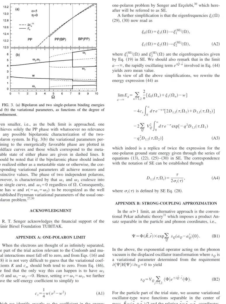
Before we close our discussions we would like to shed some insight into polaron-polaron versus bipolaron bound state energies and display the profiles of the corresponding variational parameters w and兵␻i其against the degree of con-finement. To provide an explicit track of the evolution of the ‘‘polaron-polaron’’ complex as a function of the effective dimensionality, we refer back to the simple case for which we artificially set␩⫽0, and choose␣⫽5 as a sample value being somewhat smaller than the corresponding bulk critical minimum,␣_c(3D)兩_␩⫽0⫽6.85. In Fig. 3共a兲 we plot the possible bipolaronic binding energy

E_b⫽⍀⫺E_g

accompanied by twice the binding energy of the correspond-ing scorrespond-ingle polaron over the range 0⭐⍀⭐10. To give a complementary understanding of the polaron-polaron 共PP兲 and bipolaron共BP兲 phases and the transition from one phase to the other, we also display the variational parameters as a function of ⍀ 关see Fig. 3共b兲兴. We at first note that for ⍀

⬎7.21, i.e., in the region ‘‘BP共PP兲,’’ the bipolaronic phase is

energetically more likely to show up compared to the PP phase of two individual polarons, and yet, increasing the degree of confinement enhances the stability of the BP phase. For ⍀⬍7.21, however, the state of two individual polarons is favored. In the region ‘‘PP共BP兲,’’ (4.53⬍⍀

⬍7.21) the bipolaronic phase is seen to persist rather

reces-sively where, with decreasing ⍀, the corresponding local minimum in its ground state energy starts to lose its depth and eventually diminishes for ⍀⫽4.53. When ⍀ is made

FIG. 2. The critical ratio␩cas a function of degree of

confine-ment for a succession of different␣ values. The dashed curves from bottom to top give the path-integral results obtained for ␣

⫽4,5,6,7,8,10,15,20,30. The topmost solid curve is universal for all

large␣ and has been obtained within the framework of the strong-coupling polaron theory.

even smaller, i.e., as the bulk limit is approached, one achieves solely the PP phase with whatsoever no relevance to any possible bipolaronic characterization of the two-polaron system. In Fig. 3共b兲 the variational parameters per-taining to the energetically favorable phase are plotted in boldface curves and those which correspond to the meta-stable state of either phase are given in dashed lines. It should be noted that if the bipolaronic phase should indeed be realized either as a metastable state or otherwise, the cor-responding variational parameters all achieve nonzero and distinctive values. The phase of two independent polarons, however, is characterized by that ␻1 and ␻2 coalesce into one single curve, and ␻3⫽0 regardless of ⍀. Consequently, one has w and ␯(⫽␻1⫽␻2) to be recognized as the well established Feynman variational parameters of the usual one-polaron problem.27,30

ACKNOWLEDGMENT

R. T. Senger acknowledges the financial support of the Mu¨nir Birsel Foundation TU¨ BI˙TAK.

APPENDIX A: ONE-POLARON LIMIT

When the electrons are thought of as infinitely separated, the part of the trial action relevant to the Coulomb and mu-tual interactions must fall off to zero, and from Eqs.共16兲 and

共18兲 it is not very difficult to guess that the variational

coef-ficients K and cm should both tend to zero. From Eq. 共46兲, we find that the only way this can happen is to have ␻3

→0 and␻1⫺␻2→0. Hence, setting␯⫽␻1⫽␻2, we further have the self-energy coefficient to simplify to

cs⫽ 1 4w共␯

2_⫺w2_{兲 共A1兲}

which we identify exactly as the coefficient in the energy term given by Eq. 共27兲 in a previous paper on the confined

one-polaron problem by Senger and Erc¸elebi,30 which here-after will be referred to as SE.

A further simplification is that the eigenfrequencies␰i(⍀)

共29兲, 共30兲 now read as

␰0共⍀兲⫽␰3共⍀兲→␰1 (SE)_共⍀兲,

␰1共⍀兲⫽␰2共⍀兲→␰2

(SE)_{共⍀兲, 共A2兲}

where␰₁(SE)(⍀) and␰₂(SE)(⍀) are the eigenfrequencies given by Eq. 共19兲 in SE. We should also remark that in the limit a→⬁, the rapidly oscillating term eiQជ •aជinvolved in Eq.共44兲 yields zero mean value.

In view of all the above simplifications, we rewrite the energy expression共44兲 as lim a→⬁ Eg⫽

兺

n⫽1,2 2 n关␰0共⍀n兲⫹␰1共⍀n兲⫺w兴 ⫺4cs

冕

0 ⬁ d␶e⫺w␶关2D1,1共␶,⍀1兲⫹D1,1共␶,⍀2兲兴 ⫺2

兺

Q V_Q2

冕

0 ⬁ d␶e⫺␶exp兵⫺q2D1,1共␶,⍀1兲 ⫺qz 2 D1,1共␶,⍀2兲其 共A3兲

which indeed is a replica of twice the expression for the one-polaron ground state energy given through the series of equations 共13兲, 共22兲, 共25兲–共30兲 in SE. The correspondence with the notation of SE can be established through

D1,1共␶,⍀i兲⫽

␶

2␴i共␶兲

, 共A4兲

where␴i(␶) is defined by SE Eq.共28兲.

APPENDIX B: STRONG-COUPLING APPROXIMATION In the␣Ⰷ1 limit, an alternative approach is the conven-tional Pekar adiabatic theory31which imposes a product An-satz separable in the particle and phonon coordinates, i.e.,

⌿⫽⌽共Rជ,rជ兲⫻exp

兺

Q

sQ共aQ⫺aQ †_兲兩0

_典

. 共B1兲

In the above, the exponential operator acting on the phonon vacuum is the displaced oscillator transformation where sQis a variational parameter determined from the requirement

⳵

具

⌿兩H兩⌿

典

/⳵s_Q⫽0 to yield s_Q⫽V_Q

兺

j⫽1,2

具

⌽兩e

⫾iQជ•rជj兩⌽

典

_. 共B2兲

For the particle part of the trial state, we assume variational oscillator-type wave functions separable in the center of mass, Rជ⫽(rជ1⫹rជ2)/2 and the relative rជ⫽rជ1⫺rជ2 coordinates, i.e.,

FIG. 3. 共a兲 Bipolaron and two single-polaron binding energies and 共b兲 the variational parameters, as functions of the degree of confinement.

⌽共Rជ,rជ兲⫽N exp

再

⫺1 2␭1 2_共R ␳ 2_⫹␮ 1 2_R z 2_兲

冎

⫻exp

再

⫺1₂␭2 2_共r ␳ 2_⫹␮ 2 2 rz 2_兲

冎

_共B3兲

in which Rជ_␳and Rzstand for the lateral and z components of the center of mass position vector, and the components rជ_␳

and rzhave similar meanings for the relative position vector. N is the normalization constant.

The bipolaron ground state energy can then be obtained through a numerical minimization of Eg⫽

具

⌿兩H兩⌿

典

with re-spect to the set of four variational parameters 兵␭i,␮i其 (i

⫽1,2). In computing the critical phase boundary we have

made correspondence with the results provided in a preced-ing paper32 pertaining to the strong-coupling study of the one-polaron problem consisting of the same quadratic con-finement potential.

1_{H. Haken, in Polarons and Excitons, edited by C.G. Kuper and} G.D. Whitfield共Plenum, New York, 1963兲.

2_{S.D. Mahanti and C.M. Varma, Phys. Rev. B 6, 2209共1972兲.} 3_{J. Sak, Phys. Rev. B 6, 2226共1972兲.}

4_{S.P. Kuleshov, V.A. Matveev, and M.A. Smondyrev} 共unpub-lished兲.

5_{E.A. Kochetov, S.P. Kuleshov, V.A. Matveev, and M.A.} Smondyrev, Theor. Math. Phys. 30, 117共1978兲.

6

M.F. Bishop and A.W. Overhauser, Phys. Rev. B 23, 3627

共1981兲.

7_{Y. Takada, Phys. Rev. B 26, 1223共1982兲.}

8_{H. Hiramoto and Y. Toyozawa, J. Phys. Soc. Jpn. 54, 245共1985兲.} 9_{J. Adamowski, Phys. Rev. B 39, 3649共1989兲.}

10_{T.K. Mitra, Phys. Lett. A 142, 398共1989兲.}

11_{G. Verbist, F.M. Peeters, and J.T. Devreese, Solid State Commun.} 76, 1005共1990兲.

12_{V. Cataudella, G. Iadonisi, and D. Ninno, Phys. Scr. T39, 71}

共1991兲.

13_{F. Bassani, M. Geddo, G. Iadonisi, and D. Ninno, Phys. Rev. B} 43, 5296共1991兲.

14_{G. Verbist, F.M. Peeters, and J.T. Devreese, Phys. Rev. B 43,} 2712共1991兲.

15

S. Sil, A.K. Giri, and A. Chatterjee, Phys. Rev. B 43, 12 642

共1991兲.

16_{G. Verbist, M.A. Smondyrev, F.M. Peeters, and J.T. Devreese,} Phys. Rev. B 45, 5262共1992兲.

17_{J. Adamowski and S. Bednarek, J. Phys.: Condens. Matter 4,} 2845共1992兲.

18_{A. Chatterjee and S. Sil, Int. J. Mod. Phys. B 7, 4763共1993兲.} 19_{V.M. Fomin and M.A. Smondyrev, Phys. Rev. B 49, 12 748}

共1994兲.

20_{C. Qinghu, W. Kelin, and W. Shaolong, Phys. Rev. B 50, 164}

共1994兲.

21_{F. Luczak, F. Brosens, and J.T. Devreese, Phys. Rev. B 52, 12} 743共1995兲.

22_{M.A. Smondyrev, J.T. Devreese, and F.M. Peeters, Phys. Rev. B} 51, 15 008共1995兲.

23

S. Sahoo, J. Phys.: Condens. Matter 7, 4457共1995兲.

24_{M.A. Smondyrev and J.T. Devreese, Phys. Rev. B 53, 11 878}

共1996兲.

25_{S. Mukhopadhyay and A. Chatterjee, J. Phys.: Condens. Matter 8,} 4017共1996兲.

26_{R.T. Senger and A. Erc¸elebi共unpublished兲.} 27_{R.P. Feynman, Phys. Rev. 97, 660共1955兲.}

28_{D.M. Larsen, Proceedings of the 17th International Conference} on the Physics of Semiconductors, edited by J.D. Chadi and W. Harrison共Springer, Berlin, 1985兲, p. 421.

29_{S.N. Klimin, E.P. Pokatilov, and V.M. Fomin, Phys. Status Solidi} B 184, 373共1994兲.

30_{R.T. Senger and A. Erc¸elebi, J. Phys.: Condens. Matter 9, 5067}

共1997兲.

31_{S.I. Pekar, Untersuchungen u¨ber die Elektronentheorie der} Kri-stalle共Akademie, Berlin, 1954兲.

32_{T. Yıldırım and A. Erc¸elebi, J. Phys.: Condens. Matter 3, 1271}