A Respiratory Motion Artifact Reduction Method in Magnetic Resonance Imaging of the Chest

(1)

IEEE TRANSACTIONS ON MEDICAL IMAGING. VOL. IO. NO. I , MARCH 1991 I I

A Respiratory Motion Artifact Reduction Method in

Magnetic Resonance Imaging of the Chest

Ergin

A t a l a r , Student M e m b e r , I E E E ,

and

L e v e n t O n u r a l , M e m b e r , IEEE

Abstract-A respiratory motion artifact reduction method in mag- netic resonance imaging is presented. The method is an image recon- struction algorithm based on the assumption that the respiratory motion of the chest is linear in space and arbitrary in time. The linear respiratory motion causes phase distortion on the MR data. In addi- tion, as a result of this motion, the MR data will be the samples of the Fourier transform of the spin density on a nonrectangular grid. In im- age reconstruction, before taking the inverse Fourier transform, the phase distortion is compensated and the rectangular samples are in- terpolated from the existing nonrectangular samples. Using this method, a significant amount of motion artifact suppression is achieved with a rough knowledge on the motion. In addition, it is demonstrated that the respiratory motion model parameters can he estimated using the information hidden in the motion artifacts.

INTRODUCTION

ESPIRATORY motion not only blurs the MR images but

R

also causes a ghost-like image artifact [ I ] . There are many proposed ways of eliminating this distortion [ 2 ] . The most com- monly used method is the respiratory gating [3]. In this method, data are collected during the minimum motion period. The artifact suppression is satisfactory, but the data acquisition time increases. The method known as the motion artifact suppression technique (MAST) reduces the distortion by nulling the gradient moment [4]. In this method, artifact due to the velocity term of the motion between the 90" RF pulse and the data-col- lection period (in view motion) is compensated, but the distortion due to motion between the RF pulses (view to view motion) is ignored. Another method to reduce the respiratory artifact is the respiratory-ordered phase encoding (ROPE) [ 5 ] where a respiratory signal is used to determine the order of phase encoding. This method reduces the ghost artifact, but the image blurring is still a problem. Pseudo-gating is one of the newer respiratory artifact suppression techniques [ 6 ] . Although this technique is good in reducing the ghost artifact, it also suffers from blurring.

In all of these previous studies, researchers have tried to design a new imaging pulse sequence so that the acquired MR data is the two-dimensional inverse Fourier transform of the final image. The new method we are proposing in this paper is an image reconstruction method and it can be used in conjunction with any one of the above techniques.

The motion which is linear with respect to space variables is called the linear expansion motion [7]. In this type of motion, there is no motion at the center (origin) and the amplitude of the motion is proportional to the distance from the center. On the other hand, in the block motion, the object moves as a

Manuscript received Feb. 5 , 1990; revised Aug. 6 , 1990.

The authors are with the Department of Electrical and Electronics En- IEEE Log Number 9041390.

gineering, Bilkent University, Ankara, 06533 Turkey.

whole. The respiratory motion of the chest can be assumed as a combination of both block and linear expansion motions. Throughout the text, this simplified version of respiratory motion of the chest is called linear respiratory motion. Actually, the respiratory motion is more complicated but the linear expansion and the block motions are the main components of it. For the linear respiratory motion model of the chest, the acquired data corresponds to phase-distorted nonrectangular samples of the Fourier transform domain signal of the chest image. In the proposed image reconstruction method, the phase distortion of the data is compensated and rectangular samples of the Fourier transform domain signal of the chest image are obtained by interpolating the existing nonrectangular samples. Taking the inverse Fourier transform of the new data set, a ghost-free chest image is obtained. In a previous study [8], the respiratory motion of the chest is modeled by only the linear expansion motion. Because of this reason, block motion artifacts are observed in their reconstructed image.

In addition, an iterative version of the proposed image reconstruction method is developed. It is known that the motion artifact on the image contains information on the respiratory motion and, using the proposed iterative image reconstruction method, the motion parameters can be estimated.

In the next section, the motion model of the chest is explained and the MR signal is formulated under the block and linear respiratory motion. The third section is devoted to the reconstruction method. Simulation results and sensitivity of the reconstruction method to the model parameters are explained in the fourth section. The iterative motion artifact suppression method is explained in Section V.

Throughout the text, boldface capital letters like A represent 2 X 2 matrices, boldface small letters like k stand for vectors

with two entries. The first and second entries of a vector are represented by x and y subscripts, respectively. The diagonal entries of the diagonal matrices are defined in the same way. As an example, a, and a, are the diagonal elements of the matrix A , and k , and k , are the first and second elements of the vector k . The functions which are written likef( t ) are continuous. On the other hand, the functions like

f[

n

1

are discrete.

11. FORMULATION OF THE PROBLEM The basic form of MR imaging equation is

where s, ( t ) represents the acquired MR signal in the nth imaging pulse sequence. m ( x ) is the magnitude of the transverse magnetization at position x at time 1. It is usual to assume that

(2)

12 IEEE TRANSACTIONS ON MEDICAL IMAGING, VOL. IO, NO. I , MARCH 1991

this magnitude does not change during data acquisition, so it appears as if it is time independent. In the above equation, y is the gyromagnetic ratio and g, is the gradient vector of the nth pulse sequence. Only a 90" RF pulse is considered, and the timing is relative to this pulse, i.e., t = 0 when the 90" RF pulse applied. Here, all the RF pulses are assumed to be slice- selective.

If a 180" RF pulse were applied at time T,/2, then the im- aging equation would be

If there are r 180" RF pulses, then there will be r

+

1 expo- nential functions in the integral. The integrals in these expo- nents will have alternating signs, so that the sign of the last integral will be positive. This long argument can be collected in a short imaging equation as:

where q ( t ' , t ) is 1 if the number of 180" RF pulses between time t' and t is even, else it is

-

1.

On the other hand, the two-dimensional continuous Fourier transform of m ( x ) is given by

M ( w ) =

1 1

m ( x ) exp ( -jto'x) d x .

Let M[k] be the rectangular samples of

M (

to), i.e., M [ k ] = M ( V k )

M [ k ] =

1

m ( x ) exp ( -jk'V'x) d x

where V is a diagonal sampling matrix. According to the mul- tidimensional digital signal processing theory, it is possible to reconstruct an image of the object using these samples since the object is space limited.

For a standard imaging pulse sequence, one can find proper functions for the gradients and sampling instances tkc, such that

- V k = y

1:

g k , ( t ' ) q ( t ' , t k v ) dt'. ( 7 ) See Appendix A for an example. For these gradients, the following identity is obtained [see (3) and (7)]:

S k , ( t k , ) =

W k l .

( 8 ) Therefore, the imaging equation can be rewritten as:

( 9 ) The image reconstruction method is very simple. Just take the inverse two-dimensional discrete Fourier transform of the acquired data M[k], i.e.,

m [ n ] = T - ' { M [ ~ ] } . ( 1 0 ) If the object which we are trying to monitor moves during the data acquisition period, the related imaging equation will differ

from the imaging equation (9) of the static object. Although this is the case, if one does not care about this motion, and takes the samples in the same manner as before and obtains an image by taking the inverse discrete Fourier tranform, then there will be motion artifacts on the image [ 11. These artifacts are ghost- like replicas of the moving structure. In addition, there will be blurring.

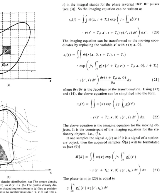
In general, there can be motion in all directions but we assume the motion is restricted to be in the selected plane, so that the excited spins are allowed to move within the selected plane, but they can never leave that plane. This assumption is acceptable for the respiratory motion in a transaxial plane of the chest. Let the time-varying magnitude of the transverse component of the magnetization at position x at time t be m ( x , t ) . (See Fig. 1 for an example time-variant proton density distribution.) Since the proton density is proportional to the f i ( x , t ) , in lit- erature sometimes m ( x , t ) is called the proton density. From now on, m ( x , t ) will be called proton density or magnitude of the transverse component of the magnetization, interchangea- bly.

Assume that our aim is to monitor the proton density at an arbitrary time, say t = 0. We labeled this specific proton density distribution by m ( x ) , i.e.,

m ( x ) = m ( x , 0). (11)

Consider an infinitesimal area element at the position xo at time to. If there is respiratory motion, then the protons in that element may move to another position. Let the function r be the position of that area element at time t .

r = r ( t ; xo, t o ) (12)

Actually, the function r is a function for time-varying coordinate transformation. A rectangular grid shown in Fig. 1 is transformed to a curve-linear coordinate system at time t . Two properties of this function will be used in the following para- graphs. The first one is the identity property of the function:

r ( t ; xo, t ) = xo.

r ( t ; r ( t 2 ; xo. t l ) , f*) = r ( t ; xo, 2 1 ) .

(13) And the second one is the transitivity property:

(14) In this paragraph, the relation between m (x, t ) and m ( x ) will be explained. Let the area of an infinitesimal rectangular region in the selected plane at the position x be d x [see the shaded region in Fig. l(a)]. The number of protons inside this region at time t = 0 is:

m ( x ) d x . ( 1 5 )

As the time goes, these protons may move. The region which contains these protons may not be rectangular. At time t , the position and the area of the differential region will be

r

( 1 ; x, 0 ) and ar ( t ; x, O)/ax d x , respectively [see the shaded region in Fig. l(b)]. Here a r ( t ; x, O)/ax is the Jacobian of r with respect to x. (See [9] for further information on the Jacobian operator.) Therefore, the total number of protons inside the region can be found as

(16) a r ( t ; X, 0 )

d x . m ( r ( t ; x, O), t ) ax

Since the number of protons is preserved, (15) and (16) must be equal. This equality gives the desired relation between m (x, t ) , and m ( x ) :

(17) ar ( t ; x, 0 )

ax . m ( x ) = m ( r ( t ; x,

o),

t )

(3)

ATALAR A N D ONURAL: RESPIRATORY ARTIFACT REDUCTION IN MRI 13

'I

(b)

Fig. 1. A time-varying proton density distribution. (a) The proton density distribution at time r = 0, m ( x ) , or A ( x , 0 ) . (b) The proton density distribution at time r , m ( x , r ) . The shaded region shown in (a) lies at position x . The protons in this region move to another position r ( r , x, 0 ) at time f.

The new region covering these protons is the shaded region shown in (b).

As the protons are moving, the gradient magnetic field applied to a proton is time dependent. Consider a proton at position x at time

r.

The gradient magnetic field that effects this proton at a previous time t' is

g, ( t ' ) r ( f ; x, t ) . ( 1 8 ) For that reason, the phase of a proton at time t is

where T, is the time between nth 90" RF pulse and 0th 90" RF pulse. T,, is added to the time variables of r because the motion must be defined with respect to a global reference. Here, this global reference is selected as the time when 0th 90" RF pulse is applied. But, in the imaging equations, the time variables are defined with respect to the current ( n t h ) 90" RF pulse. The difference between these two references is T,,. The term ~ ( t ' ,

t ) in the integral stands for the phase reversal 180" RF pulses [see (3)]. So the imaging equation can be written as

.

r ( / '

+

T,,; x ' , t

+

I-,z)

v ( r ' ,

t ) dt' d x ' . _{( 2 0 )}

)

The imaging equation can be transformed to the moving coordinates by replacing the variable x' with r

( r ;

x, 0 ) .

where &/ax is the Jacobian of the transformation. Using (17) and (14), the above equation can be simplified into the form

. r ( t '

+

T,); x, 0 ) T J ( ~ ' , t ) dt' d x . ( 2 2 ) The above equation is the imaging equation for the moving objects. It is the counterpart of the imaging equation for the sta- tionary objects, i.e., (3).

If one samples the signal s,

( r

) as if it is a signal of a station- ary object, then the acquired samples M [ k ] will be formulated as [see (9)]

1

f i [ k 1 =

5 s

t n ( x ) exp ( j y gL(t')

* r ( r '

+

TL,; x, 0 )

v ( f ' ,

r k , )

dr'

The phase term in (23) is equal to

+

y S u ' g l ( r ' ) ( r ( f '

+

Tk\; x, 0 ) - x )

v ( r ' ,

r k 8 )

d t ' . ( 2 4 ) The first term in the above equation is equal to ( - k r V r ) [see (7)]. The second term is the undesired phase added to the spins due to motion. The symbol 4 ( k , x ) represents this undesired phase term throughout this text.

'I. 5

4 ( k ,

x ) = y

So

g L ( t ' ) ( r ( t '

+

T ~ ~ ; x, 0 ) - x )

.

~ ( t ' , t k t ) dt'. (25)

Therefore, the imaging equation of a moving object can be rewritten by substituting (7) into (23):

X [ k ] =

j j

m ( x ) exp ( - j k 7 - V T x ) exp ( j 4 ( k , x ) ) d x .

(4)

IEEE TRANSACTIONS ON MEDICAL IMAGING. VOL. IO, NO. I , MARCH 1991 14

The Taylor expansion of the undesired phase term

4 ( k ,

x ) around x = xo is

where

4ho

( k , x ) stands for the higher order terms. The constant and linear terms of the expansion are as a result of block and linear respiratory motion, respectively. The block and the linear respiratory motion models are explained in the following subsection.

A. Block Motion Model

patient is modeled by

During MR data acquisition, whole body movement of the

r ( t ; x , 0) - x = f ( t ) ( 2 8 )

where the vectorf(t) is the motion function. Note that, using this model (block motion model), it is not possible to account for the rotational motion of patient. For the case where there is only the block motion, the undesired phase term,

4

( k , x ) , is independent of x . For this type of motion, the linear and higher order terms of the

4

( k , x ) are zero and the constant term is

%

4(k

xo) = Y

so

d ( t ’ ) f ( t ’

+

TkJ 77(t’, tk,) d t ’ . (29) Since

4 ( k ,

x ) is x independent, the undesired term can be taken out of the integral of the imaging equation (26), and the following result is obtained

m[kI

= exp ( j + ( k , x o ) ) ~ [ k l . (30)

Therefore, m [ k ] is a phase-distorted version of the two-di- mensional discrete Fourier transform of m ( x ) .

B. Respiratory Motion Model

modeled as follows:

The linear expansion motion around an arbitrary point is

r ( t ; x , 0) - x = F ( t ) ( x - x o ) . ( 3 1 ) This is a position-dependent motion of protons. We call this model the linear respiratory motion model. The diagonal matrix F( t ) , which brings the time dependence to the model, is called the fluctuation matrix. xo is the point where there is no motion and it is called the center of expansion. For the transaxial view of the chest, this point corresponds to the backbone. It is assumed that the left and right sides of the chest move symmet- rically. And it is also assumed that if a proton in the front part of the chest moves two units in y direction, then a proton in the center moves only one unit. In this formulation, the fluctuation functions in the x and y directions may be completely arbitrary.

Inserting (31) and (25) gives the following result:

* ( x - xo). ( 3 2 )

Therefore, if respiratory motion of the body fits the above motion model, then the undesired phase term in the imaging equation (26) will contain only the linear term [see (27)]. The constant and higher order terms will be zero.

Inserting (32) into (26) and taking the x independent factor out of the integral yield the following equation for the linear respiration model:

m [ k ] = exp ( j A k T V T x o ) M ( V ( k - A k ) ) (33) where

A k = V - I ( y

ifk‘

F ( t ’

+

T k , ) g k , ( t ’ ) ? ( t ’ , t k , ) dt‘ . (34) Here the samples of the MR signal, 312 [ k], are also the sam- ples of the phase-distorted 2-D discrete Fourer transform of m ( x ) that are taken in a nonrectangular manner. The deviation of the samples from the rectangular samples ( A k ) is a function of k .

111. RECONSTRUCTION ALGORITHM

Reconstruction of an artifact free image of an object, which has a known block motion, is relatively easy. Before taking the inverse discrete Fourier transform, a phase correction of the MRI signal is enough to obtain a good quality image:

)

There is no approximation in the reconstruction algorithm. So if the object motion exactly fits to the block motion model and if the model parameters are exactly known, then a perfect image reconstruction is possible. The above image reconstruction technique is applicable to the block motion with any function of time. A constant velocity block motion version of this reconstruction technique was previously proposed by Korin et a l .

The reconstruction algorithm of an object which has a linear respiratory motion is more complicated, but feasible as demonstrated in this paper. As it is shown in (33), the samples of the MR signal are the nonrectangular samples of the continuous Fourier transform of m ( x ) . Furthermore, the phases of the sam- ples are also distorted. The phase error of the samples are compensated using the equation

[lo].

S [ k ] = m [ k ] exp ( j A k T V T x 0 ) . (36) Here the entries of

A [ k ]

are the phase-compensated versions of the samples of the MR signal,

m[

k ] . Referring to (33) and the above equation, it is possible to write

S [ k ] =

M(

V ( k - A k ) ) . (37) Here the entries of M ( V( k - A k ) ) correspond to the non- rectangular samples of the Fourier transform of m ( x ) . To reconstruct the image, it is necessary to recover the rectangular samples of M ( u ) from its nonrectangular samples. The two- dimensional discrete inverse Fourier transform of the recovered rectangular samples will be the motion artifact free image.

In the reconstruction method, the most difficult and the most important part is the recovery of the rectangular samples of the continuous Fourier transform of the image, M ( o ) , from its nonrectangular samples.

The positions of the rectangular samples are not arbitrary. In almost all of the imaging pulse sequences, the phase encoding gradient ( 8 , ) is zero during the data acquisition period. In this period, the frequency encoding gradient ( 8,) has a nonzero value. For the case there is no motion, the acquired data in each acquisition period corresponds to the samples of M ( o ) on a line (my = w , ~ ) . Similarly if there is motion, the samples are taken on a line but at a different position and the samples on this line are taken nonuniformly

.

(5)

ATALAR AND ONURAL: RESPIRATORY ARTIFACT REDUCTION I N MRI This can be shown easily. Equation (34) can be written as:

A k , =

5"

_f,(t'

- TL) g x , k , ( t ' ) TI(?'> t k , ) d', ( 3 8 ) Ak, =

i

j;w

- TA!) g r . k , ( t ' ) TI(?'? t r , ) d t ' . ( 3 9 )

U , 0

Since there is no phase-encoding gradient and no 180" RF pulse during the data acquisition period, the above equation for A k , may be modified as:

where t , is the instant where the first data is acquired. As a result, A k v is k,-independent.

Ak., = A k , [ k x , k?.], (41

1

( 4 2 ) Ak,. = A k , . [ k , . ] .

Therefore, the sample positions on M ( w ) will look like those in Fig. 2.

Using this property, the recovery of the rectangular samples from the nonrectangular samples is reduced to two one-dimensional problems.

First, for each k v , a one-dimensional signal is defined as M k , ( w r ) = M(w,, z)!(k,.

+

A k , ) ) . (43

1

The acquired data at the k,.th phase encoding step is nonuniformly sampled.

W k r , k?.l = M r , ( z J J k r + A k , ) ) . (44) The first one-dimensional problem is the recovery of the rectangular samples of Mk, ( U , ) from its nonuniform samples.

After this step, the second one-dimensional problem must be solved. For each k.,, another one-dimensional signal is defined.

M k , ( W \ . ) = M ( t J , k , , my). ( 4 5 ) The signal Mkt ( w , ) is again sampled in a nonuniform manner. The samples are at the positions ~ , . ( k , .

+

A k , ) . The uniform samples of M A $ ( U , ) correspond to .the rectangular samples of Therefore, the two-dimensional nonrectangular to rectangular sample conversion problem can be solved by solving two one-dimensional interpolation problems.

There are many studies on one-dimensional nonuniform sampling. In 1956, Yen proved that the recovery of a band-limited signal from its nonuniform samples is possible if there is a suf- ficient number of data 1111.

Both Mk, ( m y ) and Mk> ( U , ) satisfy the requirement because

M ( o ) is the Fourier transform of a space-limited signal. Here, a method for the recovery of the uniform samples of M k , ( w , ) from its nonuniform samples will be introduced. The uniform samples of Mk, ( U , ) can be obtained in the same manner.

Using the sinc interpolation, Mk, ( w , ) can be recovered from its uniform samples as 1121

M ( w ) .

The above summation is defined for all integer k values. But M k r ( v y k ) is assumed to be zero f o r k $ [ - ( N / 2 ) , ( N / 2 ) ) for some N . The summation must be carried out for the nonzero N values.

Fig. 2. An example distribution of the nonrectangular sample positions in the M ( w ) plane. In this example, there are 10 phase-encoding steps and, in each encoding step, 10 samples are acquired. The positions of the samples are marked by cross sign. The positions of samples acquired in each phase-encoding step lie on a horizontal line. This type of sampling is a result of the respiratory motion.

But MA! ( w , ) is sampled nonuniformly at the instances U , ( k ,

+

A k , ) . Therefore, the relation between the nonuniform sam- ples and the uniform samples can be written as

M r 8 ( v , k ) sinc ( k ,

+

A k , - k ) . ( 4 7 )

- -

h t l - l N / 2 ) . l N / 2 ) )

The above equation can be converted in matrix form as

where

G(kv

+

A k , ) and

G ( k )

are the nonuniform and the uni- form sample vectors, and S is the transformation matrix. The elements of the matrix are sinc ( k ,

+

A k,. - k ) .

To calculate the uniform samples from the nonuniform sam- ples, the matrix S must be inverted.

Gk3(k)

= S - ' G k 3 ( k A

+

A k , ) (49) If the number of nonuniform samples are equal to the number of rectangular samples, then the S matrix will be a square al- temant matrix. And after a few mathematical manipulations, it can be proven that the S matrix is invertible for any set of dis- tinct k!

+

Ak!'s [13].

The matrix S may be practically singular if some nonuniform samples are too close to each other or if there is no sample around a uniform sample position. Unfortunately, this fact oc- curs frequently. To overcome this problem, the well-known singular value decomposition method is used and the uniform samples are calculated by multiplication of the pseudo-inverse of S with the nonuniform sample vector. See [ 141 for the details of the singular value decomposition and the pseudo-inversion.

Instead of solving the problem by the pseudo-inversion of the matrix, some approximate methods may be proposed. The linear and third-order Lagrange and cubic spline interpolation methods can be used if a fast image reconstruction algorithm is required. See Appendix B for the details of the above interpolation methods. The performances of the methods are compared and tested in the next section.

As a summary, in this section the block and the respiratory motion artifact free-image reconstruction algorithms are proposed. In the former, only the distorted phases of the acquired

(6)

data are compensated before taking the inverse Fourier transform. In the later one, the rectangular samples are interpolated after the phase compensation. And then the inverse Fourier transform of the calculated data gives the artifact free image.

IV. SIMULATIONS AND RESULTS

In this study, some simulations are carried out to see the properties of the proposed image reconstruction method. First, a fictitious phantom is selected as a test object. This object is assumed to have a respiratory motion. The MR signal is simulated under these conditions. The reconstruction method is tested with this MR signal. The reconstruced image has almost no blurring and motion artifact. The different interpolation methods are used in recovering the uniform samples from the nonuniform samples and their effect to image quality is observed. The new reconstruction method is tested using wrong values of model parameters. It is shown that if the error in the model parameters are reasonable, then a substantial amount of motion artifact reduction is the reconstructed image will be observed. 1n.other words, the new method is not very sensitive to the model parameters.

Let the mathematical phantom object shown in Fig. 3 be the test object. Assume that the object moves as it is defined in the linear respiratory motion model [see (3 l)]. Let the parameter x,, (the center of the linear expansion) be positioned near the backbone of the phantom. The diagonal fluctuation matrix is assumed to be

Here, the fluctuation functionf( t ) is periodic (see Fig. 4)

( 5 1 ) The amplitudes of the fluctuation function in the x and y direc- tions, a, and a,, are selected as 4 % and 10% for the simula- tions, respectively. The motion period, T,,, is assumed to be 2800 ms.

During the study, a standard spin-warp imaging pulse se- quence is applied to the test object (see Fig. 5 ) . In each simu- lation experiment, a fixed repetition time is used and T,. = 1500 ms. The echo time, Te, is 30 ms, and 256 samples are acquired with a 20 ps sampling period from each MR signal. Therefore, the data acquisition period r , = 5.12 ms. A total of 256 phase encoding steps are carried out. The time interval fx is 3 ms.

The gradient pulse amplitudes are arranged so that a region which has a size of 256 X 256 mm is viewed.

If the inverse Fourier transform were directly applied to the simulated MR signal which is taken from this moving object, then the image would have the respiratory motion artifact (see Fig. 6). The same data is reconstructed using the proposed method (see Fig. 7). The motion artifacts and blurring due to the motion are significantly suppressed.

The practical difficulty of the proposed image reconstruction method is the computational time. The most time-consuming part of the method is the interpolation from nonrectangular samples to rectangular samples. As it was explained in the previous section, to find the rectangular samples from the nonrectangular samples it is required to calculate the pseudo-inverses of ( 256

Fig. 3. The two-dimensional mathematical chest phantom. The white circular object represents the heart. The small circular objects.stand for the backbone. The lungs are represented by two elliptic objects which have different internal structures. The thin layer covering the phantom stands for the fat around the body. The proton density is given in arbitrary units. The circular objects have 1 unit of proton density, whereas the lungs have 0.1

unit. The other parts of the phantom are assumed to be filled with 0.5 units of protons density. The field of view ( f r , f , ) is (256 mm, 256 mm).

Time (seconds 1

Fig. 4. The respiratory fluctuation function which is used in the simula- tions. It is periodic with a period of T,, = 2800 ms. The function is equal to exp ( -16?/T;) for -T,,/2 < r 5 T,,/2. Tr n n G n -..G _xo... G x

-?-

-p

Fig. 5. The Fourier transform MR imaging pulse sequence used in the simulations. The repetition time, T, = 1500 ms. The echo time T , is 30 ms. 256 samples are acquired with a 20 ps sampling interval from each MR signal. Therefore, the data acquisition time rx is 5.12 ms. A total of

256 phase-encoding steps are carried out. The time interval t , is 3 ms. The gradient pulse amplitudes are arranged so that a region which has a size of

(7)

Fig. 6 . An image of the object which has a respiratory motion if a standard FT reconstruction method is used. The motion model parameters a,, a,,

xo. and yo are 4 % . IO % , 7 mm, and 98 mm, respectively. The respiratory motion artifact can be observed on the image. As a measure of the image quality, the average of the intensity levels at the outside of the region of interest, e, is evaluated as 0.121 units. The region of interest (R01) is inside the rectangle shown in the figure.

Fig. 8. An image using the linear interpolation. The rectangular samples are calculated using the linear interpolation of the nonrectangular samples. The motion artifact is reduced. The remaining motion artifacts are due to the errors in the interpolation method. The average of the intensity levels at the outside of the region of interest is 0.0548 units.

Fig. 7 . An image using the proposed reconstruction method. Almost all the motion artifacts are suppressed. The exact motion model is assumed to be known. The rectangular samples are calculated using the pseudo-inverses of 257 different matrices. The average of the intensity levels at the outside of the ROI, e , is 0.0217 units.

x 256) matrices using the singular value decomposition (SVD) method where 256 is the dimension of the image. The distribution of the nonuniform samples in each row is arbitrary. Therefore, 256 different S matrices must be decomposed. On the other hand, the positions of the nonuniform samples in each column are the same. Therefore, only one SVD is enough for the interpolation in the y direction. A total of 257 SVD are re- quired. In a SUN-3 160 system, which has a floating point ac- celerator (fpa), each SVD takes approximately 13 CPU min. Therefore, an image reconstruction time is approximately 56 h. Much quicker image reconstruction can be achieved by some other interpolation methods. The linear interpolation method requires much less computation time. First, the nonuniform samples are sorted with respect to the sampling positions. And the rectangular samples are taken from an imaginary piecewise linear curve, the comers of which are on the nonuniform samples. This method adds a total of 10 s to the conventional reconstruction time. The image obtained by this method is also acceptable (see Fig. 8). Linear interpolation is useful for reconstruction of the images which do not have much motion artifact.

Fig. 9. An image using the third-order Lagrange interpolation. The rectangular samples are calculated using the third-order Lagrange interpolation of the nonrectangular samples. Before the interpolation, 12 x 256 samples which are too close to somi other samples are removed from the nonrectangular sample set. The average of the intensity levels at the outside of the region of interest is 0.0464 units.

The third-order Lagrange and cubic spline interpolation methods are also applied. It is observed that these interpolation methods fail if there are very close samples. The noise on the neighbor samples may cause very high swings on the interpolated data. So the samples which are closer than a threshold are replaced with their averages. In a sense, this corresponds to removing singularities in the S matrix. In this way, the inter- polation method is stabilized.

The third-order Lagrange interpolation is applied after sort- ing the samples and removing the singularities (see Fig. 9). The quality of the images which are obtained using the third-order Lagrange interpolation are better compared to the images obtained using the linear interpolation. The Lagrange interpolation adds a total of 15 s to the conventional reconstruction time. The cubic spline interpolation method is best among the quick interpolation methods (see Fig. 10). The overhead of the cubic spline method is approximately the same as the Lagrange interpolation method (15 s).

As a fifth interpolation method, a composite interpolation method is used. The motion in the x direction is compensated by using the cubic spline interpolation method, and the motion

(8)

IEEE TRANSACTIONS ON MEDICAL IMAGING. VOL. IO, NO. I . MARCH 1991

Fig. 10. An image using the cubic spline interpolation. The rectangular samples are calculated using the cubic spline interpolation of the nonrectangular samples. Before the interpolation. 12 x 256 samples which are too close to some other samples are removed from the nonrectangular sample set. The average of the intensity levels at the outside of the region of interest is 0.0396 units.

Fig. 1 1 . An image using the composite interpolation. The motion in the x direction is compensated using the cubic spline interpolation. In this direction, there were not any too close samples, so all the samples are used. In the y direction. the motion compensated by the pseudo-matrix inversion. To find the pseudo-inverse, 24 eigen-values of the S matrix are set to 0. The average of the intensity levels at the outside of the region of interest is 0.0321 units.

in the y direction is compensated by the singular value decomposition. The result is almost as good as the image obtained by the motion artifact suppression using SVD in both directions (see Fig. 11). But it is much quicker (approximately 15 min).

The selection of the interpolation method among these five methods depends on the quality of the image one wants to obtain and the amount of time that can be afforded for the reconstruction of the images.

In all of the above image reconstruction methods, the exact motion model is assumed to be known. If the exact motion model is not known, then the reconstructed image will have some motion artifacts. The important point is that even if an approximate respiratory motion model is used, the reconstruction image would still be better then the image which is reconstructed by the standard methods. To test this fact, some simulations are conducted with wrong a , , a , , xo, yo, a n d f ( t ) values to observe the sensitivity of the reconstruction technique to these parameters. The cubic spline method is used in all of these simulations. And these results are also theoretically justified.

A . Sensitivity of the Reconstruction Method to the Fluctuation Function

In reality, it is not possible to measure or estimate the fluctuation matrix F ( t ) exactly. The image must be reconstructed using an approximate value for F ( t ) . The proposed reconstruction method is not very sensitive to this parameter. If one reconstructs the image of a moving object using P ( t ) instead of F( t ) , then the reconstructed image will have a similar artifact of the image of the object under a respiratory motion with the qarameter [ F ( t ) -

P ( r ) ] .

If the measurement error [ F ( t ) -

F( t ) ] is reasonable, then substantial amount of image artifact reduction is expected. This fact is justified both experimentally and theoretically.

Three simulations are carried out to observe the effect of the measurement error. F ( t ) has three parameters:

f(

r ) ,

a,, and q. The measurement error on these parameters are analyzed sep- arately. If the measurement error in the amplitude of the fluctuation function in the x direction is less than 100% (i.e., if

I

a ,

- b.,

I

<

1

a,

I

), there will be artifact suppression. In the first simulation, a , is assumed to be measured with 50% error ( 6 , =

Fig. 12. Demonstration of the sensitivity of the proposed method to the motion function amplitude a,. The image is obtained by the proposed re- construction method using fir = 2 % instead of its exact value a , = 4%. The remaining motion parameters which are used in the reconstruction are the exact motion parameters. The composite interpolation method is used. To find the pseudo-inverse, 33 eigen-values of the S matrix are set to 0. The average of the intensity levels at the outside of the region of interest is 0.0658 units.

0.5a,). And the image is reconstructed with 6, instead of a , (see Fig. 12). The ghost artifact due to motion in the y direction is completely suppressed and the artifact due to the x motion is reduced. Second, a similar simulation is carried out for the fluctuation function amplitude in the y direction. The motion artifact suppression is observed on the image which is reconstructed with 6,. = 8 % instead of its actual value of 10% (see Fig. 13). In general, if

I

a) - 6,

I

<

I

a,.

1,

then the proposed reconstruction method is helpful in the artifact reduction. In both experiments, the fluctuation function

f(

t ) is assumed to be known. An additive white noise on the measured fluctuationA function f ( t ) is assumed. The signal-to-noise ratio (SNR) o f f ( t ) is 20 dB. The image obtained b y f ( f ) is shown in Fig. 14. Since the error functionf( t ) - f ( t ) is not periodic, then A k - A k is not

periodic either, so there is no ghost-like image artifact but there is blurring on the image. As the SNR of t h e f ( t ) decreases, the contrast-to-noise ratio of the reconstructed image decreases.

(9)

ATALAR A N D ONURAL: RESPIRATORY ARTIFACT REDUCTION IN MRI 19

Fig. 13. Demonstration of the sensitivity of the proposed method to the motion function amplitude a,. The image is obtained by the proposed reconstruction method using ri, = 8 % instead of its exact value a , = 10%. The remaining motion parameters which are used in the reconstruction are the exact motion parameters. The composite interpolation method is used. To find the pseudo-inverse, 33 eigen-values of the S matrix are set to 0. The average of the intensity levels at the outside of the region of interest is 0.0761 units.

Fig. 14. The image is reconstructed using the proposed method with a white noise error in the fluctuation function. The SNR of the fluctuation function is 20 dB. The remaining motion parameters which are used in the reconstruction are the exact motion parameters. The composite interpolation method is used. To find the pseudo-inverse, 39 eigen-values of the S matrix are set at 0. The average of the intensity levels at the outside of the region of interest is 0.11 I O units.

The theoretical analysis of the sensitivity of the reconstruction method to F ( t ) is also conducted. The acquired data were formulated as [see ( 3 3 ) ]

X [ k ] = exp (-jAk'V'x,) M ( V ( k - A k ) ) . _{( 5 2 )} The proposed reconstruction method is based on this equation. M [ k ] is calculated using 311 [ k ] , before taking the inverse Fou- rier transform of M [ k ] (remember M [ k ] = M ( V k ) ) . The image reconstruction is possible if A k and x, are exactly known. In the reconstruction, if one uses A k instead of A k then the image k ( x ) will be obtained instead of m ( x ) . In this recon- struction, the following equation will be the base of the method: X [ k ] = exp ( -jAk^'V'x,) " i ( V ( k - A k ) ) . ₍₅₃₎

If the above equation is combined with ( 5 2 ) , the following re- sult will be obtained:

k(

V ( k - A k ) )

= exp ( - j ( A k - V r x 0 ) M ( V ( k - A k ) ) . (54)

Let

k

=

k - AAk. One must be careful while changing the k vector by k

+

A k , because A k and Ak are both functions of k [see (34)]. But, if one assumes that

A k [ k ] = A k [ i ] , ( 5 5 ) the following approximate equation can be obtained:

k[k]

= exp ( - j ( A k - A k ) r V'XO)

.

M ( V ( k - ( A k - A k ) ) ) . ( 5 6 )

Since the approximate equation is similar to ( 5 2 ) , the image artifact of the reconstructed image will again be a respiratory type of image artifact and the amount of this artifact will be small and proportional with the error in A k .

There is a linear relation between A k and F ( t ) :

'A,

A k = y V - '

1

F ( r ' ) g,,(t') v ( t ' , t k v ) d t ' . ( 5 7 ) Therefore, the error*in F ( t ) is proportional with the error in A k . As a result, if F ( t ) were used instead of F ( t ) as the fluc- tuation function in the reconstruction algorithm, then there would be artifacts in the reconstructed image as if there is a motion with fluctuation function F( t ) - F( t ) .

The conclusion of this discussion is that reconstruction of an image with a reasonable estimate of the fluctuation matrix F ( t ) considerably reduces the motion artifacts on the image. B. Sensitivity of the Reconstruction Method to the Offset of the Motion Model

Sensitivity discussion in this subsection is similar to the previous sections. If one reconstructs a moving object image with the motion function offset Po instead of xo, then the recon- structed image will suffer from a motion artifact. This motion artifact will be similar to the artifact of the image of an object which has a block motion with + ( k , x,) = - A k r V ( x o -

fo). A simulation result is given to confirm this argument. The reconstruction is carried out using Po instead of its real value xo

(see Fig. 15). The motion artifact on this image is similar to the motion artifact of the image of the object which has a block motion in the x-direction. A similar simulation is carried out for the offset error in the y-direction (see Fig. 16).

The sensitivity of the reconstruction method to the offset of the motion model is also theoretically analyzed. If the M R signal were taken from an object which has a respiratory motion with the motion model offset xo, then the acquired data would be as given in ( 5 2 ) . Assume that the image is reconstructed using an erroneous value of offset (Po). The relation between the Fourier domain samples of the reconstructed image and the acquired data is:

311[k] = exp ( - j A k T V 7 f o )

"i(

V ( k - A k ) ) . ( 5 8 ) If the above equation is combined with ( 5 2 ) , the following result will be obtained:

"i(

V ( k - A k ) )

(10)

Fig. 15. A simulation image to demonstrate the sensitivity of the proposed method to the motion model offset xo. The MR image is reconstructed using the proposed method using a wrong value of the offset (2, = - 3 mm, xo

= 7 m m ) . The artifact on the reconstruction image is a result of this 10 mm error. For the image reconstruction, the composite interpolation method is used. To find the pseudo-inverse, 42 eigen-values of the S matrix are set to 0. The average of the intensity levels at the outside of the region of interest is 0.0629 units.

Fig. 16. A simulation image to demonstrate the sensitivity of the proposed method to the motion model offset yo. The MR image is reconstructed using the proposed method using a wrong value of the offset (yo = -93 mm, yo

= -98 mm). The artifact on the reconstruction image is a result of this 5 mm error. For the image reconstruction, the composite interpolation method is used. To find the psuedo-inverse, 42 eigen-values of the S matrix are set to 0. The average of the intensity levels at the outside of the region of interest is 0.0715 units.

Because of the similar reasons in subsection A of this section, the vector k cannot be replaced by k

+

A k , unless we assume that

A k [ k ] = A k [ k ^ ] . (60) Then the following approximation will be obtained:

k[k^]

= exp

(

- j A k 7 V T ( f , , - xo)) M ( V ( k ^ ) ) . (61)

This equation is in the same form as (30). Therefore, the reconstructed image will suffer from the block motion if it is constructed with an approximate xo. But the amplitude of this block motion will be small and it is proportional to the error in the offset, provided that the error in the offset is smaller than the offset itself.

C. Sensitivity of the Reconstruction Method to the Higher Order Terms of the Undesired Phase

It is known that the actual respiration motion is not linear in space. For example, while the motion of the heart (for a phase of cardiac cycle) fits the block motion model, there is no motion within the spinal cord. If a linear respiration motion is used as a model of the chest motion, then the heart and spinal cord are also assumed to obey the model. Obviously, this is not true. Therefore, the question is “what will be the artifacts if the linear motion model is used for reconstructing an image of an object which has a nonlinear motion? ”.

The effects of the nonlinearity of the motion can be observed in the higher order terms of the undesired phase of the imaging equation (26)

W [ k ] =

1s

m ( x ) exp ( - j k T V T x ) exp ( j + ( k , x ) ) d x . ( 6 2 ) Although the motion model does not fit to the linear respiratory motion model, if that model is chosen for the reconstruction, then the following equation will be the relation between the acquired data and the Fourier transform of the reconstructed image.

W [ k ] = exp ( - j A k T V T x , ) k ( V ( k - A k ) ) . (63) Combining the above equation and (62) and (34), and assuming

A k [ k ] = Ak[k^] (64)

4 ( k ,

x ) = 4(k^, x ) ( 65

yield the following result:

k [ k ] =

s

m ( x ) exp ( - j k T V T x ) exp

{

j 4 ( k , x)

- A k T V ( x - x O ) } d x . _{( 66}

Since selection of A k depends on the linear respiratory model than one selects the model parameters such that

For the linear respiratory motion model which satisfies the above equality, the reconstruction method cancels the linear term of the undesired phase. If there is a constant phase term, it can be canceled by the block motion compensation technique. There- fore, (66) can be written as

k [ k ] =

11

m ( x ) exp ( - j k T V T x ) exp

{

j & , , ( k , x ) } d x . ( 6 8 ) As a conclusion, the proposed reconstruction method cancels the linear and constant terms of the undesired phase of the acquired MRI signal. If the main components of a motion is linear expansion and/or block motion, then substantial amount of motion artifact suppression will be obtained.

To observe this effect by simulation, an object which has a nonlinear respiratory motion is selected. The heart of the phan- tom (the white circular block of the phantom) is assumed to be moving as a block, while the other parts of the phantom have a linear respiratory motion. To obtain the MRI signal of this

(11)

J(1) a r A

Fig. 19. The block diagram of the proposed image reconstruction algorithm.

Fig. 17. Nonlinear motion during data acquisition causes nonlinear motion artifacts. The MRI signal is obtained by assuming the heart of the phantom has a block motion, as explained in the text while the rest of the phantom has a linear respiratory motion. The image is reconstructed by the conven- tional image reconstruction method. The average of the intensity levels at the outside of the region of interest is 0.138 units.

Fig. 18. Reconstructed image of the nonlinear motion using the proposed image reconstruction method. There is a motion artifact on the image due to the nonlinear motion of the phantom. For the image reconstruction, the composite interpolation method is used. To find the pseudo-inverse, 47 eigen-values of the S matrix are set to 0. The average of the intensity levels at the outside of the region of interest is 0.0835 units.

phantom, two simulations are carried out. The heart of the phantom is removed and two independent objects are obtained. The block motion model is used in obtaining the MRI signal of heart. Another MRI signal is obtained by assuming the remaining part of the phantom has a linear respiratory motion. The MRI signal of the phantom, which has a nonlinear motion, is acquired by adding the MRI signals of these two simulations.

The image shown in Fig. 17 is reconstructed directly by taking the inverse Fourier transform of the MR signal. On the other hand, the image shown in Fig. 18 is reconstruction by the proposed method. There is a considerable improvement in the image quality. The resultant image has some motion artifacts due to the higher order undesired phase terms.

As a result, the nonlinearity of the respiratory motion affects the reconstruction image quality. But it is demonstrated that, using the proposed image reconstruction algorithm, the effects of the constant and linear terms of the respiratory motion are compensated and a significant reduction in the motion artifact is obtained.

v.

ESTIMATION OF THE MOTION MODEL PARAMETERS

The proposed image reconstruction algorithm may be ex- pressed in block diagram form, as shown in Fig. 19.

As it is seen, for the reconstruction the motion model parameters are necessary. Three of these parameters (a,, a , , a n d f ( t ) ) may be measured using displacement transducers. The other two parameters, the coordinates of the center of expansion, ( x 0 and y o ) , may be marked by the operator on the image which has the ghost artifact.

Finding the position of the center of expansion can be auto- mated by the aid of a simple algorithm. The position of the center of expansion, (xo, yo), must be at the bottom center of the image. The location can be found from the original image which has the ghost artifact. For this purpose, the image pro- jections, p , ( ~ ) and p , ( y ) , to the x and y axis are obtained (see Fig. 20). And the estimated center of expansion is calculated. io is the mean value of X, which satisfies p , ( x )

>

T , and yo is the minimum y which satisfies p , ( y )

>

T . Here, T is an ex- perimental threshold constant. With this algorithm, the center of expansion is estimated with no error for the phantom we used. In the real experiments, there can be estimation errors. But it is already shown that the proposed algorithm is not very sensitive to the errors in the estimation of xo.

The respiratory motion measurement systems which are com- merically available cannot be used directly to obtain all of the motion parameters. In these systems, usually there is one displacement transducer and, therefore, only the fluctuation functionf( t ) can be measured. The measured motion signal is used for respiratory gating or some other respiratory motion artifact suppression methods. To calculate the model parameters a, and a,, it is not only necessary to use two transducers but it is nec- essary to know the positions of these displacement transducers. Since the ghosts on the images contain information on the motion, it is possible to overcome this practical difficulty by the aid of an estimation algorithm. An iterative method is proposed to find the motion parameters [15]. In Fig. 21, the block diagram of the iterative method is shown.

In the previous discussions, it is known that with the rough motion parameters, it is possible to reconstruct image. As the motion parameters become closer to the actual parameters, the image quality will increase. The image quality is measured by the error e . The error is the square sum of the intensities of the pixels where the object is not standing. As the error e gets closer to zero, the image quality increases. The minimization algorithm shown in Fig. 21 finds the parameters which minimize the error e . The error is a function of the estimated motion model parameters, 6, and ci,:

e = e ( & , , 6,). (69)

It is known that the reconstruction algorithm has a well behav- ior, with respect to these motion parameters (see the previous

(12)

22 IEEE TRANSACTIONS ON MEDICAL IMAGING, VOL. IO. NO. I , MARCH 1991 2.5 2 1 . 5 1 0 5 C I I I I I 50 100 150 200 250 (a) x10' 1 0 5 I 0; 50 100 150 203 250 300 (b)

Fig. 20. The projections of the image shown in Fig. 6 . (a) The projection to x-axis, p x ( x ) . (b) The projection t o y axis, p , ( y ) . The image shown in Fig. 6 is obtained by the conventional reconstruction method. p , ( x ) is ob- tained by summing the intensities of the pixels on the vertical lines. Sim- ilarly, p , ( y ) is obtained by the sum of the intensities of the pixels on the horizontal lines. The dashed line shown in both graphics represents the threshold level T .

Find the center

of expansion

I a x , Q Y

1

hlinimizr

Error

1

lniagc

Fig. 21. The block diagram for the iterative image reconstruction method. By the aid of a displacement transducer, f(r) is measured. The center of expansion (io,

yo),

is found using p , ( x ) and p , ( y ) . The remaining two motion model parameters which are necessary for the proposed reconstruction method are found by the iterative image reconstruction method. The error of the image, e , is the average of the intensity levels at the outside of the region of interest.

sections). The multivariate function e must have a global min- imum at

ci, = a,, (70)

a,. = a,. (71)

t

Fig. 22. The three-dimensional plot of the error function e(ci,,

a,).

The minimum of e function is observed at (4%, 10% ). The function is smooth. Finding its minimum is not difficult.

And no local minimum is expected. As an example, a three- dimensional plot of the error function is given (see Fig. 22). The minimum at the expected point can be seen and there is no local minimum. There are many known multivariate minimization algorithms in the literature [16]. The polytope, Powell, and quasi-Newton minimization algorithms are used to find the global minimum. The polytope algorithm solved the example problem in 160 iterations with a 0.01 % error.

On

the other hand, the Powell minimization algorithm solved the problem in 83 iterations within the same error bound. The quasi-Newton method reached the minimum in 141 iterations. The above algorithms are implemented using a SUN-3 160 workstation; each iteration took approximately 63 s.

Estimation of the fluctuation functionf ( t ) would be possible if it were periodic. But it is known that, similar to the other physiological motions of the body, the respiratory motion of the chest is quasi-periodic. And it is difficult to represent the motion with a small number of parameters. Hence, the measurement off( t ) is recommended.

As the number of unknown parameters increases, the image reconstruction time increases but the cost of additional instrumentation setup decreases. To choose the best method, the cost of instrumentation and time spent for reconstruction must be compared.

VI. CONCLUSION

In this work, a respiratory motion artifact reduction method in MR imaging of the chest is proposed. The respiratory motion of the chest in a transaxial cross-section is assumed to be linear with respect to space variables. Under this assumption, it is demonstrated that the acquired data correspond to nonrectangular samples of the phase-distorted Fourier transform of the spin density on the cross-section of the chest. The proposed reconstruction method has three steps. The first step is the compensation of the phase distortion on the samples. The second step is the interpolation of the samples on a rectangular grid using the samples on the nonrectangular grid. A motion artifact free chest image can be obtained in the last step by taking the inverse Fourier transform of these calculated samples.

Using this image reconstruction method, all the respiratory motion artifacts can be suppressed if the respiratory motion fits

(13)

model which is used in the reconstruction. But it is shown that, with an approximate respiratory motion model of the chest, a substantial amount of reduction in the motion artifact is obtained, as well.

The proposed image reconstruction method does not require any specific imaging pulse sequence. It can be used with any Fourier transform pulse sequence. Therefore, this method will increase the motion artifact suppression capability of the other standard respiratory motion artifact suppression methods. The cost is a small amount of increase in the image reconstruction computation.

The proposed image reconstruction method requires a knowledge on the respiratory motion of the chest during the data acquisition period for perfect reconstruction. This motion can be measured using a special design or can be estimated from the acquired MR data itself. We believe that both methods are feasible.

APPENDIX A

In general, the MR signal s , ( t ) was formulated as [see ( 3 ) ]

Let h ( t ) be a bandlimited signal and let { t i : i = 1 *

. .

N }

be an arbitrary set of time instances. Without loss of generality, one may assume ti L tj if i

>

j . Let & ( t ) be the signal which is obtained by the interpolation of { h ( t i ) : i = 1

. . .

N } .

Linear interpolation is defined as

where

( 7 7 )

The linear interpolation may be called first-order Lagrange interpolation.

The third-order Lagrange interpolation is defined as

L ( t )

= ( 7 8 )

t i + 2 2 t i + , , i = 1, 2 * N - 3

(0 otherwise. ( 7 2 )

For the spin-echo pulse sequence shown in Fig. 5 , if T,

<<

T I (i.e., all the spins are relaxed before each 90” RF pulse) and if T ,

>>

t , , then

The cubic spline is an interpolation method for smooth functions. Each time segment [ t, + I

. . .

t , ] is interpolated by a third- order polynomial function,

&,

( t ) . The coefficients of these functions are calculated SO that

6ctJ

= h ( f , ) ( 7 9 ) k ( t , + J = h ( t , + , ) ( 8 0 ) ( 8 1

1

m ( x ) = p ( x , y ) e - T * I T 2 ( x , \ ) . ( 7 3 )

Since, all the MR samples are taken after the 180” RF pulse

and

v

( t ’ , t ) is independent from t. It can be written as

_6:

_{( t , )}₌

_&:-

_{, ( t , )} -1 for t‘

<

T , / 2 ,

(74) 1 f o r t ’ L T , / 2 .

Let the sampling matrix V be diagonal

( 7 5 ) and let N X N be the image size in pixels.

Using simple algebra, it is possible to find the gradient amplitudes and the sampling function which satisfies ( 7 ) . The fol- lowing will be the solution:

APPENDIX B

where & l ( t ) is thefirst derivative of & ( t ) . As a boundary con- dition, &( t ) and & +

,

( t N ) are assumed to be zero. For cubic spline interpolation, the function &( t ) is defined as

( 8 3 ) h, t , + , L t

>

ti, i = 1 , 2 * N - 1

0 otherwise. & ( t ) =

For the details of these interpolation methods, refer to [ 141. ACKNOWLEDGMENT

The authors would like to acknowledge the valuable com-’ ments of Prof. Z . H. Cho.

REFERENCES

[ l ] C . Schultz, R. Alfidi, A. Nelson, S . Kopiwada, and M . Clampitt, “The effect of motion on two-dimensional Fourier transform magnetic resonance images,” Radiology, vol. 152, pp. 117-121, July 1984.

[2] M. Wood and R. Henkelman, “Suppression of respiratory motion artifacts in magnetic resonance imaging,”