Real estate and mortgage crisis : a study on the United States

(1)

REAL ESTATE AND MORTGAGE CRISIS A STUDY ON THE UNITED STATES

A Master’s Thesis by BĐLGE KARATAŞ Department of Economics Bilkent University Ankara May 2009

(2)

(3)

(4)

The Institute of Economics and Social Sciences of

Bilkent University

by

BĐLGE KARATAŞ

In Partial Fulfilment of the Requirements for the Degree of MASTER OF ARTS in THE DEPARTMENT OF ECONOMICS BĐLKENT UNIVERSITY ANKARA May 2009

(5)

I certify that I have read this thesis and have found that it is fully adequate, in scope and in quality, as a thesis for the degree of Master of Arts in Economics.

---

Assistant Prof. Dr. Taner Yiğit

Supervisor

---

Associate Prof. Dr. Fatma Taşkın

Examining Committee Member

---

Associate Prof. Dr. Zeynep Önder

Examining Committee Member

Approval of the Institute of Economics and Social Sciences

--- Prof. Dr. Erdal Erel

(6)

ABSTRACT

Karataş, Bilge

M.A., Department of Economics Supervisor: Asst. Prof. Dr. Taner Yiğit

May 2009

Like every asset price boom, the US Real Estate Boom expanded the economy until the burst occurred. Although the existence of an “irrational” boom was apparent, it has been questioned whether the increase suggested a bubble. This thesis analyzes the evolution of the US Real Estate Crisis and suggests that the real estate price increase was a bubble. A time series analysis is performed for the years 1990-2006, using monthly data on the US house prices, consumer prices, income per capita, population, unemployment rate, mortgage rate and housing starts. The results indicate that consumer prices and income per capita explain the trend in the housing prices, prior to the bubble. During the bubble, except population the fundamentals fall short in explaining the housing prices.

(7)

ÖZET

GAYRĐMENKUL VE MORTGAGE KRĐZĐ

AMERĐKA BĐRLEŞĐK DEVLETLERĐ ÜZERĐNE BĐR ÇALIŞMA Karataş, Bilge

Mastır, Ekonomi Bölümü

Tez Yöneticisi: Yrd. Doç. Dr. Taner Yiğit

Mayıs 2009

Her varlık fiyat patlaması gibi, ABD Emlak Fiyatları Patlaması da ilk etapta ekonominin genişlemesine sebep oldu. Her ne kadar "mantıksız" patlamanın varlığı belli olsa da, bu artışın balon olup olmadığı sorgulanmıştır. Bu tez ABD Emlak krizinin geçirdiği evrimi analiz etmekte ve emlak fiyat artışının balon olduğunu göstermektedir .Araştımada 1990-2006 yılları için ampirik zaman serisi analizi, ABD ev fiyatları, tüketici fiyatları, kişi başına düşen gelir, nüfus, işsizlik oranı, ipotekli konut oranı ve yeni konut sayıları aylık verileri kullanılarak yapılmıştır. Analizin sonucu tüketici fiyatları ve kişi başına düşen gelirin konut fiyatlarındaki balon eğilimi öncesinde konut fiyatlarındaki artışı açıklardığını göstermektedir. Konut fiyatları balonu sırasında, nüfus haricinde temel hiçbir indikatörün konut fiyat artışı üzerinde etkisi yoktur.

(8)

TABLE OF CONTENTS

ABSTRACT ... iii

ÖZET ... iv

TABLE OF CONTENTS ... v

LIST OF TABLES ... vi

LIST OF FIGURES ... vii

CHAPTER I: INTRODUCTION ...… 1

CHAPTER II: THE EVOLUTION OF THE REAL ESTATE CRISIS... 4

II.1. First Phase of the Real Estate Crisis... 4

II. 1. 1. Indicators of the Bubble ... 7

II.1.1.1. The Affordability Index... 7

II.1.1.2. House Prices to Rents Ratio... 8

II.1.1.3. House Prices and Consumer Prices... 9

II.2. Second Phase of the Real Estate Crisis... 11

II.3. Third Phase of the Real Estate Crisis... 16

CHAPTER III: LITERATURE REVIEW ON BUBBLES... 21

CHAPTER IV: EMPIRICAL ANALYSIS: The Relation Between House Prices and Consumer Prices... 26

IV.1. Model... 26

IV.2. Data... 27

IV.3. Results... 28

IV.3.1. Results for the period 1990-1999... 30

IV.3.2. Results for the period 2000-2006... 32

CHAPTER V: POLICY IMPLICATIONS... 35

CHAPTER VI: CONCLUSION... 37

SELECTED BIBLIOGRAPHY... 39

APPENDIX 1... 42

(9)

LIST OF TABLES

1. Heteroskedasticity and Autocorrelation Consistent OLS for

1990-1999 ... 31 2. Heteroskedasticity and Autocorrelation Consistent OLS for

(10)

LIST OF FIGURES

1. Homeownership Rate for the USA (1965-2005) ... 6

2. Housing Affordability Index for the USA (Jan 2003-Aug 2007)... 8

3. US House Prices to Rents Ratio (Jan 2000-Aug 2007) ... 9

4. Ratio of Case & Shiller Index to Consumer Price Index (Jan 1990-Sep 2007) ... 10

5. OFHEO House Price Index History for the USA (1990 Q1-2007 Q2) .11 6. Federal Reserve Short Term Funds Rate (1990-2007)…... 13

7. Adjustable-Rate Mortgages Delinquencies and Foreclosures (1998-2007) ... 14

8. Early Payment Defaults... 15

9. Quarterly Housing Vacancy Rate for the US (1995 Q1-2007 Q3)... 16

10. New Housing Units Started in the USA (Jan 2000-Aug 2007)... 17

11. Construction Expenditures in the US (1993-2007)... 17

12. Nominal and Real National Average Contract Mortgage Rates (Jan 1995-Sep 2007) ... 23

(11)

CHAPTER I

INTRODUCTION

With the crash of the US mortgage market in the beginning of 2007, high amount of financial companies declared their bankruptcy and many financial market leaders have experienced considerable decreases in their stock prices which have also affected global stock markets. Mortgage crisis has not only affected financial firms with poor lending standards but also created serious consequences for the whole US economy.

After the stock market boom and bust and terrorist attacks in the United States in 2001, when the GDP growth was only 0.5%, the economy started to recover again with the increase in investment which has had positive impact on both employment and consumer demand. Rising real estate prices has made a huge contribution in regaining the economic activities through high level of consumer confidence and improved economic expectations.

However the increase in real estate prices was far more than the inflation rate. According to the S&P/Case-Shiller Home-Price Index, house prices in the US increased by 124% between 1997 and 2006. This was one of the main indicators that

(12)

the rise in the house prices could have been a “bubble”, which has been defined by Kindleberger (1987) as:

a sharp increase in the price of an asset or a range of assets in a continuous process, with the initial rise generating expectations of further rises and attracting new buyers – generally speculators interested in profits from trading in the asset rather than its use or earning capacity”.

During a house price bubble, homebuyers think that a home that they would normally consider too expensive for them is now acceptable purchase because they will be compensated by significant further price increases (Case and Shiller, 2003: 299-362).

Various economists analyzed this phenomenon in the US and have come to different conclusions. According to Case and Shiller (2003: 299-362), the rise in housing prices clearly indicated a housing bubble. On the other hand McCarthy and Peach (2005), made counter argument that the high house prices were not off the line considering the fundamentals. This question has been answered in view of the sub-prime mortgage crisis in the beginning of 2007 that has affected not only US economy but the global society. Actually, Shiller had been arguing that there would be epic decline in house prices. He said “People think that home prices go up a lot, but home prices in 1990 were at about the same level as in 1890.” (Fox, 2007).

According to Allen and Gale (2000: 236-255), asset bubbles have three district phases: The first phase is the expansion of credit with the increase in lending which is the result of financial liberalization followed by the central bank. With the increase in lending, asset prices (such as real estate or stock) start to increase. In the second phase the rise continues for several years until the burst of the bubble leading to a collapse in the asset prices. Bursting happens when people’s expectations about

(13)

the future prices start to change. In the third phase many agents that have borrowed to buy these assets at inflated prices start to default, leading to banking and foreign exchange crises. Thus, the burst of the bubble affects the whole economy by disruption in financial and real activity (output reduction, deflationary pressures) and this can last for several years. The U.S.A. has entered the third stage in February 2007, when the subprime mortgage crisis became the headline issue with the high rates of delinquencies and foreclosures.

In this thesis, the US mortgage crisis is analyzed, with a further focus on providing an empirical analysis on capturing the refraction in the correlation between increase in the house prices and consumer prices.

The remainder of this thesis is as follows: In the second chapter the evolution of the mortgage crisis is summarized by dividing the crisis in the three phases that have been described by Allen and Gale. The third chapter reviews the literature about asset and real estate bubbles. The fourth chapter focuses on the analysis which attempts to capture the change in the pattern of the percent increase in house prices and to empirically show that the effect of consumer prices on house prices disappears with the start of the bubble. For this purpose, the model by Case and Shiller (2003) is employed, using monthly time series data for the U.S. economy between 1990 and 2006. Policy Implications will be proposed in the fifth chapter and the conclusion will be given in the sixth chapter.

(14)

CHAPTER II

THE EVOLUTION OF THE MORTGAGE CRISIS

II.1.First Phase of the Real Estate Crisis: The Start and Growth of Bubble

From the beginning of 2001, Federal Reserve started to follow expansionary monetary policy with the cut in the short term Fed Funds rate by half a percentage point, to 6%. In addition, after the dotcom burst and terrorist attacks, with the fear of deflation Fed continued cutting the interest rates until they reached 1% in 2003 which was the lowest rate of 45 years. The main reason for this policy was to avoid more severe downturn and panic in the financial system by injecting ample liquidity in to the markets (Belke and Wiedmann, 2005). It has been known that high liquidity increases the chances of bubbles. Volatility of stock markets has made returns to property more attractive encouraging a portfolio shift from equities to real estate. With low interest rates, homebuyers can comfortably service bigger mortgages and support higher house prices, resulting in an increasing demand.

On the other side of the phenomenon there has been an increase in the sub-prime mortgages starting from the mid-1990s. Sub-sub-prime mortgages are loans made to borrowers who are perceived to have high credit risk, often because they lack a

(15)

strong credit history or have other characteristics that are associated with high probabilities of default (Bernanke, 2007). This distinction can be made by looking at the loan to value (LTV) and debt service to income (DTV) ratios. Borrowers who have DTIs above 55% or LTVs over 85% are likely to be considered sub-prime (Kiff and Mills, 2007) and they are demanded higher interest payments, generally 2 percent higher, than prime borrowers. Sub-prime market has become active with the introduction of adjustable-rate-mortgages1 in 1982. In 1986, the Tax Reform Act left residential mortgages as the only consumer loans on which the interest was tax deductible. This made home equity withdrawal a preferred means of financing home improvements and personal consumption relative to other forms of consumer loans. Besides this, automated underwriting 2 has led to easier credit scoring with technological advances and securitization3 made the mortgages easily tradable with the introduction of mortgage-backed securities. These improvements have helped the development of the sub-prime mortgage market by relaxing of the credit rationing of the borrowers who were previously considered too risky by lenders (Kiff and Mills, 2007).

Thus with the increase in sub-prime lending there has been a considerable increase in the homeownership rate4 since the households that might not reached the resources before have easy access to the mortgages (Figure 1). Non-conforming sub-prime mortgages have rapidly taken the place of the mortgages that are guaranteed

1

Interest rate is periodically adjusted based on an index, for the U.S.A. it can be LIBOR, COFI, MTA, etc. This suggests that payments of borrower may change (in the interest rate resets).

2_{Underwriting is done to determine risk-based price by looking at the credit history and LTVs of the}

borrowers.

3

Securitization which allows intermediaries to pool large number of mortgages and to sell the resulting cash flows to investors has separated the original lender from borrower who is the ultimate bearer of credit risk.

4_{The number of owner-occupied housing units is divided by the number of occupied housing units or}

(16)

by Federal Housing Association (FHA) which has less flexibility and low lending limits. By 2006, only 51% of mortgage loans were conforming loans (requires detailed credit history) and the remaining part was consisting of Alt-A, a category between prime and sub-prime mortgages, and sub-prime loans both of which contain high delinquency risks.

Figure 1: Homeownership Rate for the USA (1965-2005)

Source: U.S. Census Bureau

The increase in the mortgage borrowing has led to a rise in the demand for houses. However, the supply side of the industry cannot respond immediately to the increased demand due to the time lag of new construction. Thus, real estate market is mainly driven by demand factors, at this case by low interest rates. Therefore this has led to the increase of the house prices.

(17)

II.1.1. The Indicators of the Bubble

There are various indicators that can be taken into account in order to decide if the increase in the real estate prices in the US showed bubble symptoms. In this part the most crucial three indicators are discussed: The Affordability Index, the ratio of house prices to rents and the relation between house prices and consumer prices.

II.1.1.1. The Affordability Index

From the definition of Realtors, Affordability Index shows the ability of a median income household to afford the payments of a mortgage loan. For this index 100 means that the household has enough income to pay the down payments and monthly mortgage payments of the mortgage loan. If the index is above 100, then the median income household has more than enough income to afford the mortgage payments. (National Association of REALTORS)5 From Figure 2, although the affordabilty index has been above 100, it has been decreasing gradually since 2003. The decrease from January 2003 to August 2007 is 22% which means that debts of median income households have been incresing relative to their income.

5_{The index takes both fixed-rate-mortgages and adjustable-rate-mortgages into account and calculates}

(18)

Figure 2: Housing Affordability Index for the U.S.A. (Jan 2003-Aug 2007)

Source: Research Division of the National Association of REALTORS

II.1.1.2. House Prices to Rents Ratio

House prices to rents ratio has the same intuition as the price to earning ratio, known as “Gordon Equation”: The market value of an asset is determined by the present risk adjusted discounted value of its expected income stream.6 So, the price of a house should reflect the future benefits of ownership which is indicated by rental income earned by a landlord or the implicit rent saved by an owner-occupier (The Economist, 2003). If Price/Rents ratio is high, meaning the house prices are increasing faster relative to rents, then the houses are bought because of the expectation of future increase in the prices. In the US there has been a divergence between house rents and prices, the ratio reached its highest value in May 2006 with 6 g i g E P t t − + + = ρ δ(1 )

Where Pt is the price of the asset, Et is the earnings, δ is percentage share of earnings, g

is the growth rate of earnings, i is the risk-free interest rate and ρ is the risk premium. This equation indicates that the price of an asset should rise as the risk-free interest rate and/or risk premium falls. (IMF World Economic Outlook, 2000:78-79)

(19)

83% (see Figure 3), which clearly indicates that individuals buy houses for speculative reasons. These buyers do not base their investment decisions on future income streams from rents but on higher resale price at a future date.

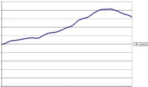
Figure 3: US House Prices to Rents Ratio (Jan 2000- Aug 2007) (2000=100)

0 0,2 0,4 0,6 0,8 1 1,2 1,4 1,6 1,8 2 ja n-00 ap r-00 jul-0 0 okt-0 0 ja n-01 ap r-01 jul-0 1 okt-0 1 ja n-02 ap r-02 jul-0 2 okt-0 2 ja n-03 ap r-03 jul-0 3 okt-0 3 ja n-04 ap r-04 jul-0 4 okt-0 4 ja n-05 ap r-05 jul-0 5 okt-0 5 ja n-06 ap r-06 jul-0 6 okt-0 6 ja n-07 ap r-07 jul-0 7 TIME P /R R A T IO Series1

Sources: Standard&Poor’s Case-Shiller Index and U.S. Bureau of Labor Statistics CPI, Rent of Primary Residence (all urban consumers)

II.1.1.3. House Prices and Consumer Prices

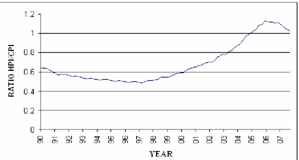
Former to the housing bubble, it has been said that house prices and inflation tended to move parallel. However, the dramatic increase in the house prices has broken down this relationship between consumer prices and house prices. Figure 4 depicts the monthly trend of the ratio between the house price index to the consumer price index, for the period between January 1990 and September 2007.

(20)

Figure 4: Ratio of Case & Shiller House Price Index to Consumer Price Index (January 1990-September 2007)

Sources: Standard&Poor’s Case-Shiller Index and U.S. Bureau of Labour Statistics CPI (all urban cons)

It can clearly be seen from this figure that after 2000, the increase in house prices outweighed the increase in consumer prices. The house prices doubled the consumer price index in 2005, when the house prices reached the peak. Further empirical focus is given to this relationship in the succeeding chapters.

Consequently, these indicators precisely suggest that there have been fundamental misalignments in the US real estate market.

(21)

II.2. Second Phase of the Real Estate Crisis: The Peak and Burst of the Bubble

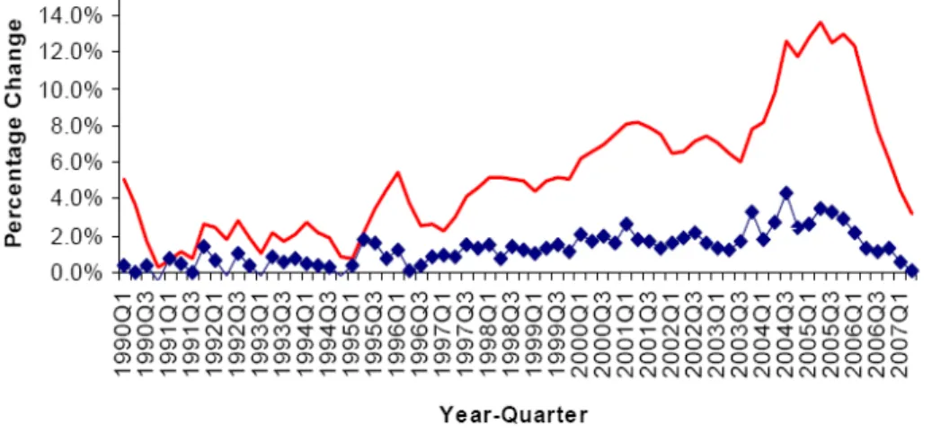
Office of Federal Housing Enterprise Oversight (OFHEO) conducts various researches on the house prices and publishes house price index for the U.S.A. every quarter7. According to the report of OFHEO the house prices in the United States has increased by 50.76% in five years as of June 2007. The yearly appreciation of the house prices was 10%. For second quarter of 2005, where the appreciation reached its peak, the annualized growth of the prices was 14.05 %.

As credit becomes more freely available, there is a positive wealth effect: if lenders increase their loans relative to house values and borrowers’ incomes, the negative effect of rising property prices on first-time buyers’ spending will fall. Homeowners can borrow or refinance non-housing debts using the increased collateral value of their property.

Figure 5: OFHEO House Price Index History for the USA (1990 Q1-2007 Q2)

Source: Office of Federal Housing Enterprise Oversight (OFHEO)

7

(22)

The increase in the prices led to huge gains in the US economy until its rapid burst. Despite the sharp fall in share prices and a worldwide plunge in industrial production, business investment and profits, consumer spending has held up relatively well, supported by low interest rates and the wealth-boosting effects of rising house prices. Boosting wealth not only increased spending, but also allowed owners to borrow more against the rising value of their homes (The Economist, 2002).

The number of housing starts jumped from 1.5 million at an annual rate in August 2000 to a peak 2.3 million in January 2006. In 2005, housing construction accounted for 6.2% of GDP which was the highest rate since 1950 (The Economist, 2007). This has also led to increasing employment rates in the real estate market. Real estate, residential construction and three other housing related Labor Department job categories together add up to 6.6% of U.S. employment. They accounted for 46% of the new jobs created in the U.S. between January 2001 and May 2006 (Fox, 2007).

Also, financial markets gained a lot from the housing bubble. According to Wall Street Journal, from 2004 to 2006, more than 2500 banks, thrifts, credit unions and mortgage companies made a combined $1.5 trillion in the risky high-interest-rate mortgage loans.

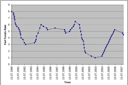
This positive image, however, did not last long. In 2004, Federal Reserve started to increase its short term funds rate gradually from 1%, until it reached to 5.25% in June 2006 (see Figure 6). As Shiller (2000) argued, tightened monetary

(23)

policy, which was the rise in the interest rates, is associated with the bursting of the bubbles.

Figure 6: Federal Reserve Short Term Funds Rate (1990-2007)

0 1 2 3 4 5 6 7 8 9 1 3 .0 7 .1 9 9 0 1 3 .0 7 .1 9 9 1 1 3 .0 7 .1 9 9 2 1 3 .0 7 .1 9 9 3 1 3 .0 7 .1 9 9 4 1 3 .0 7 .1 9 9 5 1 3 .0 7 .1 9 9 6 1 3 .0 7 .1 9 9 7 1 3 .0 7 .1 9 9 8 1 3 .0 7 .1 9 9 9 1 3 .0 7 .2 0 0 0 1 3 .0 7 .2 0 0 1 1 3 .0 7 .2 0 0 2 1 3 .0 7 .2 0 0 3 1 3 .0 7 .2 0 0 4 1 3 .0 7 .2 0 0 5 1 3 .0 7 .2 0 0 6 1 3 .0 7 .2 0 0 7 Time F e d F u n d s R a te

Source: Federal Reserve

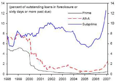
With the slow-down in the increase of the house prices and the upward movement in the interest rates on both fixed and adjustable rate mortgages in 2006, there has been a rapid deterioration in the mortgage loans originated in 2006. Formerly, rising house prices combined with low interest rate levels made prepayment easy for distressed borrowers since their equity had an increasing value. However, increased monthly payments and decreased equity value forced subprime borrowers to default on their payments. The rise in deliquencies has led to the rise in the foreclosures. In the fourth quarter of 2006, about 310,000 foreclosure proceedings were initiated. However the quarterly average for the previous two years was 230,000. In the second quarter of 2007, almost 3% of subprime loans entered foreclosure (The Economist, 2007).

(24)

Figure 7: Adjustable-Rate Mortgages Delinquencies and Foreclosures (1998-2007)

Source: Citigroup

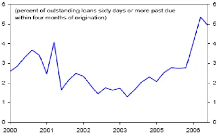
As the underlying pace of mortgage originations began to slow, but with investor demand for securities with high yields still strong, some lenders evidently loosened underwriting standards. So-called “risk-layering”, combining weak borrower credit histories with other risk factors, such as incomplete income documentation or very high cumulative LTV, became more common. These looser standards were likely an important source for the rise in "early payment defaults"(see Figure 8)--defaults occurring within a few months of origination--among subprime ARMs, especially those originated in 2006 (Bernanke, 2007).

(25)

Figure 8: Early Payment Defaults

Source: Credit Suisse and Loan Performance

The improvements in the mortgage market that are mentioned before has also increased the rates of deliquencies in the market. With securitization assesing the risk was particularly difficult when risky mortgages were packed into securities that combined other types of risk profiles. Hence, lenders have bought mortgage-backed securities not knowing the risk they entailed. Mostly banks with subprime-specialist subsidiaries and speciality finance companies have adversely affected from subprime crisis. Since mid-2006, some non-depository, poorly capitalized firms representing 40% of 2006 subprime originations have closed down operations, declared bankruptcy or been bailed out (Kiff and Mills, 2007).

Foreclosures have led to an increase in the vacancy rates because owners have had to leave their properties. As can be seen from the Figure 9, the housing vacancy rate for the US has started to rise sharply since the second quarter of 2006, with the increase in the delinquency rates.

(26)

Figure 9: Quarterly Housing Vacancy Rate for the US (1995 Q1-2007 Q3) 0 0,5 1 1,5 2 2,5 3 1995 Q1 1995 Q3 1996 Q1 1996 Q3 1997 Q1 1997 Q3 1998 Q1 1998 Q3 1999 Q1 1999 Q3 2000 Q1 2000 Q3 2001 Q1 2001 Q3 2002 Q1 2002 Q3 2003 Q1 2003 Q3 2004 Q1 2004 Q3 2005 Q1 2005 Q3 2006 Q1 2006 Q3 2007 Q1 2007 Q3 TIME V A C A N C Y R A T E Series1

Source: U.S. Census Bureau (Based on current population survey)

II.3. Third Phase of the Real Estate Crisis: The Impacts on the Economy

The rise in the demand on houses, forced the supply side of the market to become active. New constructions have increased rapidly until 2006. While demand was beginning to decline, homebuilders were still running at a high speed. Because of the time lag between demand and supply in the real estate industry, the slowing down in construction, which can be clearly seen from the decline in the number of housing starts (the number of new constructions), in Figure 10, has started in the second quarter of 2006.

(27)

Figure 10: New Housing Units Started in the U.S.A. (Jan 2000- Aug 2007)

Source: U.S. Census Bureau

The impact of the diminished demand on the supply side of the economy can also be observed by the decrease in the construction expenses (Figure 11). The hit in construction also hit the labor market. According to the Labor Department (2007), job creation had lurched into reverse after four years of gains.

Figure 11: Construction Expenditures in the US (1993-2007)

(28)

The defaults on the subprime mortgages have decreased the reliability of the mortgage backed securities. Major lenders as Countrywide Financial have tightened the credit conditions and avoided sub-prime lending. Overall sub-prime originations were down by 50 percent from the second quarter of 2007. Not only mortgage lenders and thrifts as Washington Mutual have incurred considerable losses, but also major banks such as Citigroup, brokerage firms such as Merrill Lynch, the two government sponsored mortgage-finance firms Fannie Mae and Freddie Mac have been severely hit by the mortgage crisis (Isidore, 2007).

Banks raised 3-month interbank rates, because they lack the confindence to loan money to one another. The credit squeeze has raised market interest rates which made harder for distressed borrowers to finance. Since August 2007, Fed has injected liquidity to the markets to ensure their smooth functioning. Besides this, Fed has also decreased the short-term fed funds rate by 0.75% to 4.50% to overcome the adverse affects of the credit crunch.

The tighter credit conditions leads to a deeper and more protracted housing downturn then assumed. This would extend the decline in the residential investment and put great downward pressure on the household finance and consumption.

Consequently, the reduction in household and construction spending and the increase in the unemployment, has been rising from 4.4% in April 2007 to 4.7% in September 2007, will further weaken the growth of GDP, which had grown only by 0.9% in the first quarter of 2007. In addition, RealtyTrac, a company that tracks foreclosures, has estimated up to 1.5 million households has entered the foreclosure

(29)

process in 2007, double 2006's figure, and with some 2.5 million adjustable-rate mortgages resetting to higher rates before the end of 2008 (The Economist, 2007).

Rising delinquencies on these so-called sub-prime home loans in the US were infecting a broad swathe of markets around the world at an alarming pace. Northern Rock and the Clemos were swept up in the global credit crisis. The reason of this widespread effect of mortgage crisis is the securitization that has made trading the mortgages easily while spreading their risks all over the world to prevent major financial institution from collapsing. It has also tied far-flung markets more closely together. That means a crisis in a niche market in one country can contaminate lots of other markets that at first glance have little to do with each other. Technology transfers information in seconds, giving the infection a more potent scope (Barr, 2007). For instance the M&G Investment Management, which is a London-based investment firm, expects $400 billion andScottish Widows Investment Partnership, with almost $200 billion in assets, experienced that blow-up firsthand on 20th of August 2007.

The first effect of the sub-prime mortgage backed securities on the overseas emerged in July 2007 when German bank IKB Deutsche Industriebank AG was bailed out by state-owned KFW Group. Three months later German savings banks rescued Sachsen LB. In addition to these incidents some of the world’s most known banks (besides Citigroup) as HSBC and ABN Amro has lent huge amounts of money to money market managers who have been trying to fight with the sub-prime crisis. In the UK the situation was not different Barclays PLC had to finance Cairn High Grade Funding, an investment vehicle and HBOS PLC lent a huge amount of money

(30)

to Grampian. The Bank of England had given billions of pounds in emergency loans to Northern Rock to keep it afloat.

(31)

CHAPTER III

LITERATURE REVIEW ON BUBBLES

In regard to property bubbles Robert Shiller is one of the major researchers in this area. He made his name in the 1980s by attacking the notion that “the stock market rationally reflects the true value of the companies whose shares are traded on it” (Fox, 2007). In March 2000, he analyzed the stock market bubble in his book “Irrational Exuberance”. “Irrational Exuberance” which means wishful thinking on the part of investors is often used to describe a heightened state of speculative fervor. The phrase was first used by Alan Greenspan at the Annual Dinner and Francis Boyer Lecture of The American Enterprise Institute for Public Policy Research in December 5, 1996. His words were

...sustained low inflation implies less uncertainty about the future, and lower risk premiums imply higher prices of stocks and other earning assets. We can see that in the inverse relationship exhibited by price/earnings ratios and the rate of inflation in the past. But how do we know when irrational exuberance has unduly escalated asset values, which then become subject to unexpected and prolonged contractions as they have in Japan over the past decade?”

These words indicate that there could be speculative bubble in the stock market and a possibility of a decline in stock prices.Immediately after those words, the stock market in Tokyo, which was open as he was giving this speech, fell sharply,

(32)

and closed down 3% and Hong Kong fell by 3%. Then markets in Frankfurt and London fell by 4%. The stock market in the US fell by 2% at the open of trade. The strong reaction of the markets to Greenspan's seemingly harmless question was widely noted, and made the term irrational exuberance famous.

Shiller (2000), mentions psychological factors that affect people’s decisions: “People do not even know to any degree of accuracy what the “right” level of market is: not many of them spend much time thinking about what its level should be or whether it is over/under priced today.” There is a “money illusion” in the markets that people take into account nominal interest rates rather than real interest rates as happened in the real estate market. In addition he also indicates that speculative bubble cannot grow forever, when demand decreases then the growth in the asset prices stop.

These psychological factors were also apparent in the mortgage market. Because of the bubble concerns in the media, Case and Shiller (2000)8 conducted a survey in several cities of the US and found out some interesting results about the homeowners point of views regarding the housing market. 90 percent of the homeowners expected an increase in the future house prices and they did not perceive themselves in the middle of bubble even at the height of the bubble. In addition, homeowners indicated that they have found investment on house is safer than investing on stocks and they have changed their portfolios from stock market to real estate markets. They indicated that nominal interest rates are the most important reason for them to decide on buying the house. Economists have been arguing on this

8_{Survey has been done on 2000 individuals, who bought new houses between March and August}

(33)

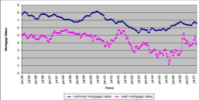
issue, because although nominal interest rates were low, since the inflation level was also low, real interest rates on mortgages were high. However, as this survey suggests while borrowing, households take nominal interest rates into consideration. Figure 12 shows the movement of monthly nominal and real average contract mortgage rates for the years between 1995 and 2007. Although the nominal rates have followed a stationary path during this period, the real mortgage rates were highly volatile and they have increased dramatically in the last two years. Thus the “money illusion” clearly showed itself in the mortgage market.

Figure 12: Nominal and Real National Average Contract Mortgage Rates (January 1995- September 2007) 0 1 2 3 4 5 6 7 8 9 ja n -9 5 ju l-9 5 ja n -9 6 ju l-9 6 ja n -9 7 ju l-9 7 ja n -9 8 ju l-9 8 ja n -9 9 ju l-9 9 ja n -0 0 ju l-0 0 ja n -0 1 ju l-0 1 ja n -0 2 ju l-0 2 ja n -0 3 ju l-0 3 ja n -0 4 ju l-0 4 ja n -0 5 ju l-0 5 ja n -0 6 ju l-0 6 ja n -0 7 ju l-0 7 Time M o rt g a g e R a te s

nominal mortgage rates real mortgage rates

Sources: Mortgage-X and Inflationrate.com

Other major studies in these fields are the ones conducted by Case, Quigley and Shiller (2001) and Case and Shiller (2003). Case, Quigley and Shiller (2001), looked at the relationship between increases in housing wealth, financial wealth, and consumer spending. They have conducted a panel data analysis firstly with 14 countries using annual data in the years between 1975 and 1999 for various periods.

(34)

Secondly they used a panel with quarterly data of US states for the years between 1982 and 1999. The estimation has been done by relating consumption to income and wealth measures. The results suggest that mainly for the United States, the real estate market is more important in determining the consumption behavior of households than the stock market. Accordingly, wealth effect is stronger in real estate market. This suggests that when the house prices increase consumers increase their spending much more than the effect of an increase in the stock prices.

The study by Case and Shiller (2003) has also related house prices with income. They have done empirical research and conducted a questionnaire survey to find out the symptoms of the bubble. Their empirical research was based on defining house prices by looking at the major economic indicators as population, employment, number of housing starts, income per capita, mortgage rate and unemployment rate. Their research focused on prices – volatile states for the period 1985-2002. They have found that income explains the changes in the house prices and during the period 2000-2002 they could not reject the null hypothesis that a bubble existed in the states that they have studied.

On the other hand, McCarthy and Peach (2005) arrived to the conclusion that there was no bubble in the housing market in United States. The main argument that they have based their reasoning was that OFHEO house price index is not a truly “constant quality” index which means that the increases in this index could have been caused by the increase in the quality of the houses. Thus, although they have found an increase in the price/rents ratio, they argued that, OFHEO index was misleading. Besides this, they also argued that the decrease in the interest rates has

(35)

created a doubt of bubble. Thus without taking into account the other considerations, as the dramatic increase in the mortgage lending, in house prices in major states, in the construction expenditures and expectations, and basing their reasoning on a not supported argument, they came in to the suspicious conclusion that there was no house price bubble.

(36)

CHAPTER IV

EMPIRICAL ANALYSIS: The Relation Between House Prices and

Consumer Prices

It has unambiguously been observed in various empirical papers that the increase in house prices tended to move parallel with the increase in consumer prices, prior to 1999 (Lansing, 2008). However, the dramatic rise in the house prices from 2000 onwards ceased this parallel relationship. To analyze this refraction, an empirical analysis is conducted in this chapter.

IV.1. Model

The analysis of this thesis is based on the study by Case and Schiller (2003). In an attempt to ameliorate their model, several modifications have been made. First of all, instead of using quarterly data, monthly data is employed. In search of the relation between house prices and consumer prices, the monthly percentage change in consumer prices is included. Furthermore, the variable employment has been eliminated from the model. Lastly, the entire period is divided into two time periods

(37)

in order to capture the structural break in the end of 1999. The first period runs from January 1990 until December 1999, and the second period starts from January 2000 and lasts until December 2006. This break follows logically from the fact that the bubble has started in the beginning of 2000.

The model that is analyzed is denoted by equation (1):

(1) t t t t t t t

ntRate

Unemployme

gStarts

Hou

te

MortgageRa

Population

come

PersonalIn

CPI

HPI

ε

β

+

∆

=

∆

5 4 3 2 1 0

sin

%

It is hypothesized that a positive correlation exists between the increase in the house prices and consumer prices in the first period, January 1990 - December 1999, that the expected coefficient for the change in the CPI is positive and significant. In the second period, from January 2000 until December 2006, it is expected this relationship to break, meaning that previously positive and significant coefficient becomes insignificant in the second period. This will indicate that the consumer prices do not have any influence on the movement of house prices. Additionally, it is expected that the macroeconomic indicators also will fall short in explaining the house price growth for the second period analysis. The rationale for this expectation is to prove the movement in the house prices was solely directed by speculative and psychological factors rather than by the movement in the economic indicators.

IV.2.Data

In order to estimate the model (1), monthly data is employed for the time period from January 1990 until December 2006. The total number of observations is

(38)

204. The dependent variable is measured as the monthly percentage change in the house prices which are taken from the Standard & Poor’s Case-Shiller Index.

One independent variable is the percentage change in the Consumer Price Index, which is taken from U.S. Department of Labor Bureau of Labor Statistics. The data reflects all urban consumers and is seasonally adjusted. Another regressor is the variable Personal Income and Its Disposition, which is seasonally adjusted at annual rates and is measured in billions of dollars. The data is from the National Accounts provided by the Bureau of Economic Analysis, U.S. Department of Commerce. Thirdly, population data are retrieved from the U.S. Bureau of Economic Analysis, measured in thousands of individuals. Fourthly, the Civilian Unemployment Rate is collected from the U.S. Department of Labor: Bureau of Labor Statistics. The data is seasonally adjusted, and is measured in months in percentages, for individuals of age 16 and older. Fifthly, seasonally adjusted at annual rates data on Housing Starts is taken from the U.S. Department of Commerce: U.S. Census Bureau. Lastly, our measure for the mortgage rate as expressed in percentages is the National Average Contract Mortgage Rate which is taken from the Mortgage-X, Mortgage Information Website.

IV.3.Results

Empirical analysis departed from employing an OLS regression measuring the percentage change in house prices using the fundamentals mentioned above (and denoted in equation 1). First, in order to verify the assumption of the existence of the

(39)

structural break, a representative regression of the model for the whole sample period, between 1990 and 2006 has been conducted. (Appendix Table A1). Chow Breakpoint test is done for the first month of 2000 in order to clarify the structural break (can be seen in the Appendix, Table A2) The P-value of the test is 0.00 indicating that the null hypothesis of no structural change in the house price changes before and after January 2000 is rejected.

Second, since the analysis involves time series, at this point it is important to test for serial correlation. The Durbin- Watson test statistic from the representative regression shows a low value (0.30) indicating that there exists first-order autocorrelation in the model. In order to test for higher order correlation, Breusch-Godfrey Serial Correlation LM test is conducted with including lags up to 2. The test rejected the null hypothesis of no serial correlation. Table A3 in Appendix depicts the correlogram of squared residuals, from which it can be seen that there is autocorrelation and partial correlation. Following these indications, the analysis on two different periods is done with second order autoregressive process and second order moving average error processes, i.e. ARMA (2,2). Before analyzing the results, it is crucial at this point to test the structural break with Wald test by using the regressions of two different time periods.

The validity of the Chow test is limited because it assumes the variances of residuals in two sub-samples are equal. Thus it is convenient to conduct the structural break test with Wald test in case the residual variance is different. The null hypothesis is no structural break with a Chi-square distribution.

(40)

The Wald test is constructed as:

(2) W =

(

b₁−b₂

) (

' V₁+V₂

) (

−1 b₁ −b₂

)

Where b₁ and b₂ are coefficient vectors for two estimated models and V₁and V₂ are the covariance matrices for the models. Using E-views, Wald test is 56.69, the probability of Chi-square distribution with eleven degrees of freedom is 0.00 suggesting that the null hypothesis of no structural break is rejected. In the next sub-sections the results of the two regressions are going to be analyzed in detail.

IV.3.1. Results for the period 1990 – 1999

The OLS regression results for the period 1990-1999 have been tested for the existence of heteroskedasticity. White-test rejected the null hypothesis of homoskedasticity with a P-value of 0.003. Accordingly the regression is done by controlling both for heteroskedasticity and autocorrelation –using Newey-West Errors. Because of the change in the method, it is crucial to conduct the Wald-test for structural break for the heteroskedasticity and autocorrelation consistent regression results, the test again has been conducted in the same way as before and the P-value again rejects the null of no structural break for the results between two regressions. The results thereof for the first sub-sample are depicted in Table 1.

(41)

Table 1: Heteroskedasticity and Autocorrelation Consistent OLS for 1990-1999 Dependent Variable: PERHPI

Method: Least Squares

Sample (adjusted): 1990M03 1999M12 Included observations: 118 after adjustments Convergence achieved after 27 iterations

Newey-West HAC Standard Errors & Covariance (lag truncation=4) MA Backcast: 1990M01 1990M02

Coefficient Std. Error t-Statistic Prob.

PERCP 0.241077 0.138367 1.742292 0.0843 INCOME 0.196018 0.043923 4.462767 0.0000 POP -5.342663 3.565874 -1.498276 0.1370 RNMAR 0.042684 0.062966 0.677892 0.4993 START -1.30E-05 0.000249 -0.052378 0.9583 UNEMP 0.067321 0.073281 0.918661 0.3603 C -4.011484 1.895126 -2.116738 0.0366 AR(1) 1.666425 0.050323 33.11455 0.0000 AR(2) -0.915740 0.047538 -19.26326 0.0000 MA(1) -0.824079 0.125567 -6.562835 0.0000 MA(2) 0.270024 0.152405 1.771759 0.0793

R-squared 0.882377 Mean dependent var 0.164080

Adjusted R-squared 0.871384 S.D. dependent var 0.547250

S.E. of regression 0.196260 Akaike info criterion -0.330164

Sum squared resid 4.121439 Schwarz criterion -0.071880

Log likelihood 30.47970 Hannan-Quinn criter. -0.225293

F-statistic 80.26874 Durbin-Watson stat 2.003309

Prob(F-statistic) 0.000000

Inverted AR Roots .83-.47i .83+.47i

Inverted MA Roots .41+.32i .41-.32i

The adjusted R-squared of the regression is 0.87, which indicates a reasonable fit. The table reveals that the percentage change in consumer prices is significant at 10% level and has a positive coefficient indicating that a 1% increase in the consumer prices increases house prices by 0.24%. This result supports the expectation that prior to the rapid increase in the house prices, consumer prices and house prices were positively correlated. Personal Income has highly significant and positive coefficient indicating an increase in the income increases house prices since it increases the demand for houses. Other fundamentals do not prove to have significant effects on house prices. Population variable has a negative and

(42)

insignificant coefficient which does not give a rational interpretation. Mortgage rate as well has insignificant and wrong signed coefficient since it is expected that an increase in the mortgage rate would decrease the house prices instead of increasing them. Housing starts do not have a coefficient significantly different from zero, thus the influence of this variable on house prices do not exist. The unemployment rate has a low coefficient which is insignificant. Positive and significant AR(1) suggests an increase in house prices mostly depends on the previous periods. AR(2) is significant but has a negative coefficient. Additionally, both of the moving averages are significant, although the first moving average has a negative sign. Thus, the percentage increase depends on both first and second past errors. This shows an important characteristic of the house price changes: one can explain house prices by looking at the previous pattern of the house prices besides income and the percentage increase in the consumer prices.

IV.3.2 Results for the period 2000 – 2006

The regression for the second sample period has been conducted again using the Newey-West Error corrected regression since the White-test for this sub-period again represented heteroskedasticity (Table A4; Appendix). The performance of the regression for this time period is depicted in Table 2.

(43)

Table 2: Heteroskedasticity and Autocorrelation Consistent OLS for 2000-2006

Dependent Variable: PERHPI Method: Least Squares Sample: 2000M01 2006M12 Included observations: 84

Convergence achieved after 31 iterations

Newey-West HAC Standard Errors & Covariance (lag truncation=3) Backcast: 1999M11 1999M12

Coefficient Std. Error t-Statistic Prob.

PERCP -0.171559 0.117465 -1.460513 0.1484 INCOME -0.082342 0.054533 -1.509939 0.1354 POP 18.08159 8.530006 2.119763 0.0374 RNMAR -0.139839 0.108134 -1.293200 0.2000 START -0.000160 0.000168 -0.953437 0.3435 UNEMP 0.297155 0.156899 1.893925 0.0622 C 1.495635 1.953847 0.765482 0.4465 AR(1) 1.388923 0.164839 8.425929 0.0000 AR(2) -0.581516 0.153438 -3.789921 0.0003 MA(1) -0.085163 0.176717 -0.481919 0.6313 MA(2) 0.315298 0.152851 2.062775 0.0427

Sum squared resid 3.319449 Schwarz criterion 0.187085

Log likelihood 16.51191 F-statistic 60.95796

Durbin-Watson stat 1.927873 Prob(F-statistic) 0.000000

Inverted AR Roots .69-.32i .69+.32i Inverted MA Roots .04+.56i .04-.56i

In this regression adjusted R-squared is 0.88, which represents same level of goodness of fit with the first sub-sample regression. As was expected, the positive and significant coefficient of the percentage change of the CPI is replaced by a negative and insignificant coefficient in this period. This shows that the behavior of the house price increase cannot be explained with the increase in the consumer prices. Additionally the positive coefficient of income becomes insignificant and negative. Thus this variable falls short in explaining the pattern of the house prices. In this regression, population has a significant effect, 5%, on the change of the house prices

(44)

indicating that an increase in the population increases the house prices. However the other variables cannot explain the change in the house prices. Mortgage Rate has negative and insignificant coefficient; the coefficient of Housing Starts is insignificant and close to zero. The unemployment rate, however, has a significant coefficient at 10% level but has a positive sign, which does not make sense in explaining house prices. Furthermore, it is found that AR(1) and AR(2) are significant, suggesting that an increase in the house prices cannot be explained by any fundamentals ( except population), but its previous realizations.

Thus, the empirical analysis represented in this part proves the hypothesis that the increase in consumer prices cannot explain the increase in the house prices after 2000, after the housing bubble started. The positive and significant coefficient of CPI for the first sub-period becomes negative and insignificant in the second period. Furthermore, it has been found that the following independent variables do not have the expected influence house price increases; unemployment rate, mortgage rate, and housing starts. Consumer prices and income per capita influence the housing price increase before the bubble; population influences the increase in the house prices after the bubble. The influence of income has also been encountered in the study done by Case and Shiller (2003). However, they have found that only income explains the trend in the house prices, whereas in this study the influence of the consumer prices has also been apparent. Since Case and Shiller (2003) do not include CPI in their analysis the findings regarding CPI cannot be compared9.

9

In order to see the relationship between the change in the house prices and consumer prices, a regression has been conducted with using only inflation rate as the independent variable explaining the percentage change in the house prices. That analysis shares the same conclusion with the regression conducted in this thesis that the positive coefficient of inflation rate in the first sub-period becomes negative and insignificant in the second sub-period.

(45)

CHAPTER V

POLICY IMPLICATIONS

Based on the empirical results, one can derive a number of policy implications to attempt to accommodate the negative effects of the mortgage crisis. To begin with, the market turbulence has caused investors to lose their confidence in financial markets. Additionally, banks have increased inter-bank rates, because they fear the exposure to risks on the sub-prime mortgage market. In order to change these developments, one has to reestablish the confidence of investors. Although this is an uncontrollable factor, the Fed attempts to regain trust by liquidity injections and interest rate reductions. Additionally, one would be able to regain trust by enhancing the transparency of financial institutions.

To alleviate the individuals who are negatively affected by the current crisis, a program of loan restructuring has been designed. However, some critics have argued that this would worsen the crisis by artificially propping up the home prices. If foreclosures occur without intervention, the market would recover faster, since decreasing house prices make them affordable to buyers. If instead the adjustable mortgage rates are shifted to prime mortgage rates -which are much lower than

(46)

ARMs-, then the interest payments will become more affordable to sub-prime borrowers. According to the Federal Reserve Bank of Boston, half of the sub-prime borrowers have the adequate credit scoring for a prime mortgage loan. Thus, shifting the qualified borrowers to prime rates will reduce the amount of foreclosures (Calbreath; 2007).

The current mortgage crisis has also provided policy insights that could be employed to limit the effects of any future mortgage crisis. First, in dealing with the burst of the housing bubble, one could design better forms of social insurance that allow one to manage real risks more effectively. Second, financial regulators should protect customers by imposing rules to prevent abusive practices. These arise through the intricate contracts that misinform potential customers of the payment conditions of the mortgages. Additionally, many borrowers relied on their brokers who were earning higher commission rates from sub-prime contracts (Calbreath, 2007). Financial regulators could also support potential customers through counseling and financial education for potential borrowers (Bernanke, 2007). Other protections include greater mortgage disclosures of payments over the lifetime of a loan and a greater prohibition of deceptive advertising (Sahadi, 2007).

(47)

CHAPTER VI

CONCLUSION

Although the debate on the housing price bubble has shifted to another debate concerning increasing regulation in financial markets, it is crucial to analyze the causes of the financial crisis and how the house prices started to show bubble symptoms. To this aim, the progress of the crisis has been outlined by dividing the periods of the crisis as the way it is described by Allen and Gale (2000). During the first phase, Fed’s low interest rate policy led to increased credits and demand on real estates which led to the increase in house prices. The indicators have pointed that house prices cannot be explained by any other parameters than people’s expectations. A considerable portion of the increase in house prices can be explained by psychology as Shiller (2000) pointed out. In the second phase positive effects of bubble and the burst of the bubble has been explained. Third phase has showed the crash in the financial market because of the tightening in the lending. Focusing on the bubble literature, the regression model by Case and Shiller (2003) has been ameliorated and employed. The monthly data for the period 1990-2006 is divided into two periods, before and after housing bubble, to indicate the break of the relation between house price increase and consumer price increase. The results have suggested that for the first period -besides income and the past realizations of the

(48)

lagged dependent variable and error terms- the inflation rate has a positive and significant effect on the house price increase. The second period analysis has showed the break in this relationship and led one to conclude that except population, none of the fundamentals can explain the sudden growth rate in the house prices.. Consequently, the results of the thesis confirm the findings by Case and Shiller (2003) and Case, Quigley and Shiller (2001) that the increase in the US housing prices was indeed a real estate price bubble which busted in the first months of 2007, leading to a mortgage crisis and credit crunch, whereof the effects are still spreading throughout the world.

(49)

SELECTED BIBLIOGRAPHY

Allen, F. and Gale, D. January, 2000. “Bubbles and Crises,” The Economic Journal Vol: 110: 236-255

Baker, Dean. June, 2006. “Is the Housing Bubble Collapsing?: 10 Economic

Indicators to Watch,” Center of Economic and Policy Research, Issue Brief, Washington D.C.

Barr, A. November 17, 2007. “Toxit Export,” Market Watch.

Belke, A. and Wiedmann M. September/October, 2005. “Boom or Bubble in the US Real Estate Market?,” Intereconomics 40, 5; ABI/INFORM Global, p:273.

Bernanke, Ben. May 17, 2007. “The Subprime Mortgage Market”, Board of Governors of the Federal Reserve System, Speech.

<http://www.federalreserve.gov/newsevents/speech/bernanke20070517a.htm>

Calbreath, D. December 9, 2007. “Bush’s plan on mortgage problems isn’t enough,” Sign on San Diego.com.

Case, K.E., Quigley, J.M., and Shiller, R.J. November, 2001. “Comparing Wealth Effects: The Stock Market versus The Housing Market”, NBER Working Paper 8606, JEL No. E2,G1.

Case, K.E. and Shiller, R.J. 2003. “Is There a Bubble in the Housing Market?”, Brookings Papers on Economic Activity. ABI/INFORM GLOBAL No.2: 299-362.

Case&Shiller Home Price Index. August, 2007 Standard and Poor’s.

<http://www2.standardandpoors.com/portal/site/sp/en/us/page.topic/indices_c smahp/2,3,4,0,0,0,0,0,0,3,1,0,0,0,0,0.html>

(50)

Civilian Unemployment Rate. September 29,2008. Federal Reserve Bank of St. Louis.

<http://research.stlouisfed.org/fred2/series/UNRATE/downloaddata?cid=12 >

Consumer Price Index. 2008. U.S. Department of Labor Bureau of Labor Statistics. <http://www.bls.gov/cpi/>

Economic Indicators. 2007. U.S. Census Bureau.

<http://www.census.gov/cgi-bin/briefroom/BriefRm> Federal Reserve Fed Funds Rate. 2007. <www.federalreserve.gov>

Fox, J. September 13, 2007. “Coping with a Real-Estate Bust,” Time.com

Greenspan, A. December 5, 1996. “The Challenge of Cental Banking in a Democratic Society,” Federal Reserve Board.

Housing Affordability Index. August, 2007. National Association of Realtors. http://www.realtor.org/Research.nsf/Pages/HousingInx

Housing Starts. 2007. U.S. Census Bureau Economic Indicators. < http://www.census.gov/cgi-bin/briefroom/BriefRm>

Inflation Rates. 2007, www.inflationrate.com.

International Monetary Fund. May, 2000. “Asset Prices and the Business Cycle,” IMF World Outlook pp: 77-112

International Monetary Fund. October, 2007. “Globalization and Inequality,” IMF World Outlook pp: 69-104

Isidore, C. December 11, 2007. “Americans split on mortgage bailout,” CNNMoney.com.

Kiff, J. and Mills P. July, 2007. “Money for Nothing and Checks for Free: Recent Developments in U.S. Subprime Mortgage Markets,” IMF Working Paper WP/07/188.

(51)

Kindleberger, C.P. 1987. “Bubbles,” in J. Eatwell, M. Milgate, P. Newman: The New Palgrave: A Dictionary of Economics, Volume 1, London, Maruzen

Lansing, K. June 20, 2008. “Speculative Bubbles and Overreaction to Technological Innovation,” FRBSF Economic Letter.

McCarthy, J. and Peach R.W. October, 2005. “Is there a “Bubble” in the Housing Market Now?,” Networks Financial Institute at Indiana State University, Policy Brief.

National Average Contract Mortgage Rate. 2007. Mortgage-X. <http://mortgage-x.com/x/indexes.asp>

News Release. August 30, 2007. Office of Federal Housing Enterprise Oversight. <http://www.ofheo.gov/media/hpi/2q07hpi.pdf>

Personal Income & Population. 2008. U.S. Department of Commerce Bureau of Economic Analysis.

<http://www.bea.gov/national/nipaweb/TableView.asp?SelectedTable=75&V iewSeries=NO&Java=no&Request3Place=N&3Place=N&FromView=YES& Freq=Month&FirstYear=1979&LastYear=2008&3Place=N&Update=Update &JavaBox=no#>

Sahadi, J. September 20, 2007. “Congress warned: Easy on loan fix,” CNNMoney.com

Shiller, R.J. 2000. “Irrational Exuberance,” Princeton University Press, U.S.A.

?March 28, 2002. “Going through the Roof,” the Economist. Economist.com.

?March 6, 2003. “Betting the House,” the Economist. Economist.com.

?May 29, 2003. “Castles in the Hot Air,” the Economist. Economist.com.

?October 4, 2007. “The Hammer Drops,” the Economist. Economist.com.

(52)

APPENDIX 1

Table A1: Representative Regression Results

Dependent Variable: PERHPI Method: Least Squares Sample: 1990M01 2006M12 Included observations: 204

Variable Coefficient Std. Error t-Statistic Prob.

PERCP -0.066498 0.167767 -0.396372 0.6923 INCOME 0.005257 0.018073 0.290876 0.7715 POP 8.105672 3.609613 2.245579 0.0258 RNMAR -0.135618 0.070531 -1.922806 0.0559 START 0.001183 0.000321 3.683080 0.0003 UNEMP -0.108831 0.052828 -2.060090 0.0407 C -0.656625 1.224834 -0.536093 0.5925

S.E. of regression 0.523294 Akaike info criterion 1.576365

Log likelihood -153.7893 F-statistic 26.94667

Durbin-Watson stat 0.302800 Prob(F-statistic) 0.000000

Table A2: Chow Breakpoint Test Chow Breakpoint Test: 2000M01

F-statistic 16.90083 Probability 0.000000 Log likelihood ratio 99.24161 Probability 0.000000

(53)

Table A3: Correlogram of Squared Residuals

Sample: 1990M01 2006M12 Included observations: 204

Autocorrelation Partial Correlation AC PAC Q-Stat Prob

.|***** | .|***** | 1 0.670 0.670 92.807 0.000 .|*** | *|. | 2 0.368 -0.145 121.01 0.000 .|* | *|. | 3 0.127 -0.107 124.39 0.000 .|. | .|. | 4 -0.012 -0.024 124.42 0.000 *|. | .|. | 5 -0.059 0.013 125.16 0.000 .|. | .|. | 6 -0.040 0.034 125.50 0.000 *|. | *|. | 7 -0.073 -0.117 126.66 0.000 *|. | .|. | 8 -0.087 -0.008 128.29 0.000 .|. | .|* | 9 -0.043 0.081 128.69 0.000 .|. | *|. | 10 -0.043 -0.075 129.09 0.000 .|. | .|. | 11 -0.047 -0.026 129.57 0.000 .|. | .|. | 12 -0.041 0.002 129.94 0.000

(54)

Table A3:White Heteroskedasticity Test for Period 1990-1999

F-statistic 2.199152 Probability 0.003026

Obs*R-squared 46.90476 Probability 0.010148

Dependent Variable: RESID^2 Sample: 1990M03 1999M12 Included observations: 118

C -1.356748 13.92173 -0.097455 0.9226 PERCP -3.916091 2.403387 -1.629405 0.1067 PERCP^2 0.289478 0.197908 1.462687 0.1470 PERCP*INCOME 0.085446 0.054293 1.573800 0.1190 PERCP*POP -3.850133 3.384482 -1.137584 0.2583 PERCP*RNMAR 0.192425 0.088308 2.179010 0.0319 PERCP*START 0.000195 0.000416 0.469543 0.6398 PERCP*UNEMP 0.108928 0.113552 0.959275 0.3400 INCOME -0.190831 0.682603 -0.279563 0.7805 INCOME^2 0.004439 0.009082 0.488763 0.6262 INCOME*POP -0.049382 0.653461 -0.075570 0.9399 INCOME*RNMAR 0.002708 0.020857 0.129832 0.8970 INCOME*START -6.11E-05 0.000108 -0.565252 0.5733 INCOME*UNEMP 0.009634 0.029794 0.323334 0.7472 POP -23.57301 26.07665 -0.903989 0.3684 POP^2 -48.35282 40.35480 -1.198193 0.2340 POP*RNMAR 2.237869 1.114500 2.007957 0.0476 POP*START 0.009342 0.006332 1.475543 0.1436 POP*UNEMP 0.967470 1.274543 0.759072 0.4498 RNMAR 0.484340 0.952459 0.508515 0.6123 RNMAR^2 -0.021683 0.023021 -0.941872 0.3488 RNMAR*START -0.000211 0.000171 -1.232798 0.2209 RNMAR*UNEMP -0.037987 0.043013 -0.883146 0.3795 START 0.003472 0.003925 0.884565 0.3787

START^2 -1.32E-07 4.66E-07 -0.283291 0.7776

START*UNEMP -0.000248 0.000184 -1.346376 0.1816

UNEMP 0.365511 1.226055 0.298119 0.7663

UNEMP^2 -0.006355 0.026513 -0.239678 0.8111

Sum squared resid 0.134187 Schwarz criterion -2.809302

(55)

Table A4: White Heteroskedasticity Test for Period 2000-2006

F-statistic 1.747401 Probability 0.039377

Obs*R-squared 38.40970 Probability 0.071612

Dependent Variable: RESID^2 Sample: 2000M01 2006M12 Included observations: 84

C 5.431773 72.71647 0.074698 0.9407 PERCP -9.224197 11.91504 -0.774164 0.4421 PERCP^2 0.842215 0.783053 1.075553 0.2867 PERCP*INCOME -0.013582 0.124206 -0.109348 0.9133 PERCP*POP 6.296606 33.39568 0.188546 0.8511 PERCP*RNMAR 0.695337 0.892876 0.778760 0.4394 PERCP*START 0.000342 0.001239 0.275591 0.7839 PERCP*UNEMP 0.875210 0.724916 1.207325 0.2324 INCOME 0.333150 2.360522 0.141134 0.8883 INCOME^2 -0.009806 0.028531 -0.343710 0.7324 INCOME*POP -0.501822 5.277661 -0.095084 0.9246 INCOME*RNMAR 0.012501 0.128860 0.097010 0.9231 INCOME*START -0.000132 0.000229 -0.574626 0.5678 INCOME*UNEMP 0.091310 0.130342 0.700542 0.4865 POP 250.0187 304.3254 0.821551 0.4148 POP^2 -3013.414 873.8816 -3.448309 0.0011 POP*RNMAR 35.16994 21.78616 1.614325 0.1121 POP*START -0.030385 0.050111 -0.606347 0.5467 POP*UNEMP 15.42516 15.96818 0.965994 0.3382 RNMAR -7.681548 8.864404 -0.866561 0.3899 RNMAR^2 0.250664 0.332914 0.752940 0.4546 RNMAR*START -0.000311 0.001075 -0.289391 0.7734 RNMAR*UNEMP 0.413501 0.474883 0.870743 0.3876 START 0.017949 0.017592 1.020329 0.3120

START^2 -1.29E-06 1.78E-06 -0.724742 0.4716

START*UNEMP -0.001011 0.001013 -0.998715 0.3222

UNEMP -5.234676 7.561370 -0.692292 0.4916

UNEMP^2 0.073662 0.266263 0.276650 0.7831

S.E. of regression 0.282782 Akaike info criterion 0.572923