New signal representation based on the
fractional Fourier transform:
definitions
David Mendlovic, Zeev Zalevsky, Rainer G. Dorsch, and Yigal Bitran Faculty of Engineering, Tel Aviv University, 69978 Tel Aviv, Israel
Adolf W. Lohmann
Department of Physics of Complex Systems, Weizmann Institute of Science, 76100 Rehovot, Israel
Haldun Ozaktas
Faculty of Electrical Engineering, Bilkent University, Turkey
Received January 25, 1995; revised manuscript received June 7, 1995; accepted June 27, 1995 The fractional Fourier transform is a mathematical operation that generalizes the well-known Fourier trans-form. This operation has been shown to have physical and optical fundamental meanings, and it has been experimentally implemented by relatively simple optical setups. Based on the fractional Fourier-transform operation, a new space-frequency chart definition is introduced. By the application of various geometric op-erations on this new chart, such as radial and angular shearing and rotation, optical systems may be designed or analyzed. The field distribution, as well as full information about the spectrum and the space – bandwidth product, can be easily obtained in all the stages of the optical system. 1995 Optical Society of America
1.
INTRODUCTION
The name of this paper was originally “Linear phase-space representation based on the fractional Fourier transform”; however, we changed the title because the term phase space means different things to different people. We did not want to create wrong expectations, yet we feel that the main concept is still best explained if we use the loosely defined term “phase space,” taking into account that, in the text below, phase-space repre-sentation means space-frequency reprerepre-sentation.
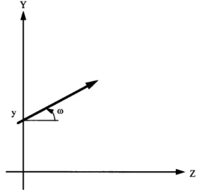
Phase-space representations are useful tools for dual time-frequency analysis, image compression, data pro-cessing, and also designing and analyzing optical systems. For optical implementations, the well-known Yv repre-sentation considers light as a bunch of rays, although each ray has a spatial location and direction (see Fig. 1). These two parameters are represented as a coordinate in the Yv plane. Thus the Yv chart has two axes, one for presenting the spatial coordinate y and the other for the angle of the ray’s propagation v, i.e., the derivation of the first coordinate. Note that two-dimensional rays are translated to a four-dimensional Yv chart. One of the greatest disadvantages of such a representation is that the ray model does not take into account the diffraction effects; thus the output result is only a ray approxima-tion of the light propagaapproxima-tion.
Another type of phase-space representation is the Wigner transform.1 The Wigner transform is a
mathe-matical operation applied to the input field distribution
fsxd: Wf fsxdg Wsx, nd Z ` 2` f √ x 1x 0 2 ! f p √ x 2x 0 2 ! 3 exps22pinx0ddx0. (1)
This transform represents the spatial and the spec-tral properties of the function simultaneously, taking into account diffraction phenomena as well. However, this transform suffers from the fact that it is not linear (but bilinear). Thus sometimes it is not convenient to use this transform with linear systems.
Reconstruction of a function from its Wigner chart can be done with fsxd 1 f ps0d Z ` 2` W √ x 2 , n ! exps2pinxddn . (2) However, there is an uncertainty factor of a phase co-efficient when the inverse Wigner transformation is performed.
For analyzing and synthesizing optical systems, the Yv and the Wigner representations provide various promis-ing properties. The elementary optical operators, free-space propagation and multiplication with a lens, are expressed as X-shearing and Y -shearing transforma-tions (see Fig. 2), respectively, applied on the input field displayed in one of these phase-space representations. Thus these tools may overcome the intensive use of com-plicated chirp integrals in the optical design process, and both the field distribution and its spectrum can be obtained immediately from the phase-space presentation. Below we present a novel phase-space representation that may be advantageous in various cases. We call this representation thesr, pd chart. This representation can be used for designing optical systems and provides prop-erties similar to those of the Yv and Wigner representa-tions. Also the field and its spectrum at different planes can be easily extracted, and elementary optical systems, such as free-space propagation or a lens, cause simple op-erations that we call radial shearing or angular shearing
Fig. 1. Schematic illustration of the Yv representation.
Fig. 2. Schematic illustration of X- and Y -shearing.
of the new representation. Because it is a linear repre-sentation, it is easily reversible and it takes into account diffraction effects. As is shown in Section 2, this repre-sentation involves the fractional Fourier transform (FRT ), a linear transformation that generalizes the conventional Fourier transform and that was recently introduced to the optics community.
Section 2 gives the relevant details about the FRT. Section 3 introduces the exact definition of the new rep-resentation, and Section 4 gives some of its mathematical properties, including the definition of the radial- and the angular-shearing operations.
An important note that is related to digital image pro-cessing and tomography applications of the FRT is the fol-lowing. Recently, a new time-frequency analyzing tool, the Radon – Wigner transform, was suggested2,3 and used
for the time-frequency representation of signals.4,5
With-out being named, this approach led exactly to a chart that contains a continuous representation of the FRT of a signal as a function of the fractional Fourier order. As we mention below, we call this representation thesx, pd chart, and it may also be useful in optics because it
ex-plicitly shows the propagation of a signal inside a graded-index (GRIN) medium.
2.
FRACTIONAL FOURIER TRANSFORM
The FRT is a new mathematical tool to be used, for ex-ample, in spatial filtering operations. The Fourier trans-form of fractional order p is defined in such a manner that the common Fourier transform is a special case with order
p 1. An optical implementation of the FRT is provided
in terms of quadratic GRIN media or in a setup that in-volves free-space propagation – lens – free-space propaga-tion or lens – free-space propagapropaga-tion – lens.
There are two common definitions for the FRT. Both definitions were proven to be identical, as shown in Ref. 6. The first optical FRT definition7 – 9is modeled as the
vari-ation of the field during propagvari-ation along a quadratic GRIN medium by a length proportional to p, where p is the FRT order.
The second definition is based on the Wigner distribu-tion funcdistribu-tion.10 This is a complete signal description
that displays time and frequency information simul-taneously.1,11
Both definitions were generalized through a transfor-mation kernel, as illustrated in Ref. 12:
hFpfusxdgjsxd Z
` 2`
Bpsx, x0dusx0ddx0, (3)
where Bpsx, x0d is the kernel of the transformation, and
it is equal (according to the first definition) to
Bpsx, x0d p 2 expf2psx21 x02dg ` X n0 i2pn 2nn! 3 Hns p 2p xdHns p 2p x0d , (4) where Hnis a Hermite polynomial of order n, or, according
to the second definition,
Bpsx, x0d exp 8 < :2i " p sgnssin fd 4 2 f 2 #9= ; j sin fj1/2 3 exp √ ipx 21 x02 tan f 2 2ip xx0 sin f ! . (5)
3.
DEFINITION
The Fourier transform of fractional order p is defined in a manner such that the classical Fourier transform is a special case with order p 1. An optical implementa-tion of the FRT is possible with quadratic GRIN media and bulk optics implementation (see Section 2 for further details). The integral definition of the FRT is
upsxd C1 Z ` 2` usx0dexp " ip tan fsx0 2 1 x2d # 3 exp √ 22pi sin fxx0 ! dx0, f pspy2d , (6)
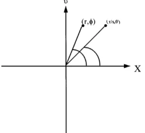
Fig. 3. Illustration of thesx, pd chart.
where p is the fractional order and C1 is a normalizing
constant that is given by
C1 exp 8 < :2i " p sgnssin fd 4 2 f 2 #9= ; j sin fj1/2 . (7)
One approach for presenting the different FRT orders with respect to the GRIN definition is a graphical chart that we call ansx, pd chart. For a one-dimensional ob-ject this plot contains two axes. The vertical axis x is the spatial one-dimensional light distribution upsxd of the
FRT order p of the original function u0sxd [as given in
Eqs. (6)]. The horizontal axis is the FRT order p (see Fig. 3 for a graphical illustration). More explicitly, one can write
Fsx, pd upsxd . (8)
As a result, in this plot all the fractional Fourier orders of the original function u0sxd are calculated and displayed
in one chart. Another point of view is that the sx, pd chart explicitly shows the propagated light distribution within a GRIN piece.7 – 9 Note that thesx, pd chart
pro-vides several interesting applications that will be de-scribed in a sequel to this paper.
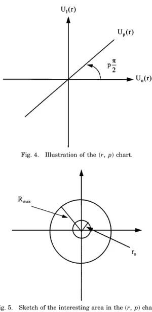
The next step for obtaining what we call ansr, pd chart is to perform a Cartesian-to-polar-coordinate transform of thesx, pd chart. Here, all the fractional Fourier orders of the function are drawn as angular vectors. Each FRT order is drawn along the r axis in specific angular ori-entation of f pspy2d, where p is the fractional order. Implicitly, one can write thesr, pd representation as
Fsr, pd upsrd . (9)
Figure 4 gives a graphical illustration of thesr, pd chart representation. It is important to note that r may get negative values. The r coordinate negative values are a by-product of thesr, pd chart definition. However, dis-cussing negative values for r does not conflict with the polar-coordinate definition because
up12srd ups2rd . (10)
Another note is connected with r 0. This singu-lar point contains no relevant information and should be avoided when the chart is used. As a polar representa-tion, the required spatial resolution for a lower r value is higher. Thus, practically, a certain area of jrj , r0is
not able to carry the necessary information (because of the limited spatial resolution of every plot) and must be avoided too. Figure 5 shows a schematic sketch of the in-teresting area of thesr, pd chart. In this figure, Rmaxis
the radius that confines the information of the fractional plane of the input object. Thesr, pd chart is our candi-date for serving as a phase-space representation. It con-tains full information about the object (along f 0) and about its spectrum [along f spy2d]. Additional infor-mation regarding the mixture space-frequency informa-tion is given along with other values of f. The inverse transformation is trivial:
upsrd Fsr, pd , (11)
and, for the object itself,
u0srd Fsr, 0d . (12)
In Section 4 several properties of the sr, pd chart are analyzed and demonstrated.
Fig. 4. Illustration of thesr, pd chart.
4.
MATHEMATICAL PROPERTIES
A. MotivationLet us recall from Lohmann10 that the FRT can be
achieved by the following two algorithms: Algorithm 1:
usx0d ) W fusx0dg Wsx, nd ) RotfWsx, ndg
) Inverse Wigner upsxd . (13)
Algorithm 2:
usx0d ) Wsx, nd ) XshearfWsx, ndg ) YshearfWsx, ndg
) XshearfWsx, ndg ) Inverse Wigner upsxd , (14)
where Rot is the rotation operation in the plane. The shearing operations are defined as
Xshearf fsx, ydg fsx 1 ay, yd ,
Yshearf fsx, ydg fsx, y 1 axd . (15)
Because the lens operation in the Wigner plane is a Yshear
and a free-space propagation is an Xshear, the procedure
described in Eq. (14) is in fact a FRT operation.
Note that similar properties are relevant also for the
Yv diagram. The fact that the common optical opera-tions (free-space propagation, lens, Fourier transform, and FRT) affect the Wigner and the Yv in relatively simple geometric transformations increased the use of these charts for analyzing and synthesizing optical systems.
Our motivation is to show that the sr, pd chart has similar properties and might be more suitable than the Wigner and the Yv charts for some applications.
B. Full Mathematical Definition
The explicit mathematical definition of thesr, pd chart is based on Eqs. (6) and (10) as follows:
Fsr, pd upsrd C1 Z` 2` usx0dexp √ pir 21 x 02 tan f ! 3 exp √ 22pi rx0 sin f ! dx0. (16)
For obtaining the conventional Fourier transform s p 1d, one should examine the distribution on the axis of f spy2d on the sr, pd chart. More generally, to obtain any other FRT order p, one should examine the chart angular distribution at an angle ofsppdy2.
Note that because the FRT definition is general enough to deal with all types of signal (complex as well), the information contained in thesr, pd chart is not restricted to the type of signal.
C. Fractional Fourier Transform Operation
Assume a function usx0d and its sr, pd chart Fsr, pd. The
sr, pd chart of uqsx0d [FRT of order q of usx0d] is
Fqsr, pd su
qdpsrd uq1psrd Fsr, p 1 qd . (17)
One can note that Fqsr, pd is a spqdy2 angular rotation
of Fsr, pd.
Thus one can conclude that performing a FRT means rotating the sr, pd chart. Algorithm (13), based on the sr, pd representation, is thus
usx0d ) Fsr, pd ) RotfFsr, pdg
) Inversesr, pd chart ) upsxd . (18) D. Lens Operation
One of the most common optical operators is a multipli-cation with a chirp function that represents a field dis-tribution of u0sx0d that passes through a lens. It can be
written as u0sx0dexpsia0px02d when a0 is related to the
lens focal length f as a0 21
l f
, (19)
where a0is a physical parameter given in units of inverse
square meters. Because the mathematical formulation has no unit, in order to use the parameter a0 there we
define a na0, where n 1 sm2d.
Our interest is to find the effect on thesr, pd chart with respect to the original chart Fsr, pd. Let us denote the new sr, pd chart as Flenssr, pd. From Eqs. (6) one can
note that Fslensdsr, pd C1 Z ` 2` u0sx0dexpsiapx02d 3 exp √ ipx0 21 r2 tan f ! exp √ 2i2p rx0 sin f ! dx0 C1exp √ ip r 2 tan f ! Z ` 2` exp 2 4ipx02 √ 1 tan f 1 a !3 5 3 exp √ 2i2p rx0 sin f ! dx0. (20)
For simplicity, let us denote b 1
tan f 1 a 1 tan u
. (21)
From well-known trigonometric equations, one obtains 1
sin u p
b21 1 . (22)
Thus, based on the scale factor
s sin u sin f, (23) Eq. (20) becomes Fslensdsr, pd C1exp √ ip r 2 tan f ! Z ` 2` u0sx0d 3 exp √ ip x0 2 tan u ! exp √ 2i2px0 rs sin u ! dx0 cuusrsd , (24)
where c is the quadratic phase factor outside the integral, and uusrsd is the s2udyp FRT order of the input function
with a scale factor of s. As a result, one can note that the effect of a lens on the sr, pd chart is a coordinate transformation. Each point inside the original chart is angularly rotated and radially scaled. The rotation u – f
Fig. 6. Schematic illustration of the shear operation in polar coordinates.
and the scale s are tan u tan f 1 1 a tan f , s 1 sin f " √ 1 tan f 1 a !2 1 1 #1/2. (25)
We call this coordinate transformation a radial-shearing transformation. The motivation for this nickname is as follows. Let us examine what a conventional X-shearing is. Graphically, according to Eqs. (15), Fig. 6 represents an X-shearing operation example. After transformation to polar coordinates, Eqs. (15) become
u tan21 √ r sin f r cos f 1 ar sin f ! , s r
fsr sin fd21sr cos f 1 ar sin fd2g1/2. (26)
A division of the first equation of Eqs. (26) by r cos f and the second by r leads to
u tan21 √ tan f 1 1 a tan f ! , s 1 sin f " 1 1 √ 1 tan f 1 a !2#1/2. (27)
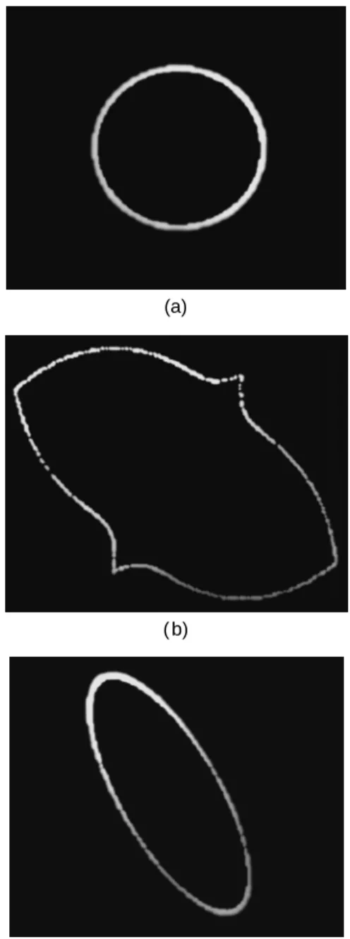
By inspection one can note that Eqs. (25) and (27) are exactly the same except that Eq. (25) relates to the scaled radius of rs [Eq. (24)], and Eqs. (27) relate to rys (Fig. 6). Those rotation and scale factors are called the radial-shearing operation. Figures 7 and 8 are com-puter simulations that illustrate this new transforma-tion operated on a square and on a circle, respectively. The radial-shearing transform was applied on two simplesr, pd charts, a square and a circle. In Fig. 7(a) the original square is shown. Figures 7( b) and 7(c) show the transformed square according to regular X-shearing and radial-shearing operations, respectively. Figure 8(a) is a circled Fsr, pd. Figures 8(b) and 8(c) show again the
regular X-shearing and the radial-shearing operations applied over this chart.
The regular X-shearing operation applied over a square turns the square into a parallelogram. When applied over a circle, the X-shearing operation turns the circle into an ellipse.
E. Free-Space Propagation
Another important optical operation is free-space propa-gation. According to the Fresnel integral, a signal u0sx0d
that propagates through the free space along a distance
z is uisx, zd exp √ i2p l z ! ilz Z ` 2` u0sx0dexp " ip lzsx02 xd 2 # dx0. (28) One can note that the propagation integral is fully equivalent to a multiplication of the spectrum of u0sx0d
by exps2iplzn2d, where n is the frequency coordinate.
Thus the free-space propagation is visualized as a rotation by 90±of thesr, pd chart, then a lens operation with a
2mlz [where m 1 s1ym2d because in our mathematical formulations we want a to be without units] is obtained, and then the sr, pd chart is rotated back by 290±. As
a result, because we have already proved that the lens operation is analogous to an X-shearing operation and is called radial shearing, the 90±rotation will force the
free-space propagation to be analogous to the Y -shearing operation of thesr, pd chart. This operation is called an angular-shearing operation.
F. Space– Bandwidth Product Calculation
So far we have investigated the effect of various optical op-erations on thesr, pd chart. In this subsection we show another piece of information that can be extracted from the sr, pd chart: the space–bandwidth product (SW) of the signal. In many cases, the knowledge of the SW is critical for the analysis and the design of optical systems. In general, obtaining the SW is relatively complicated and contains space and frequency calculations. Using the ef-fect of a lens and free-space propagation on the sr, pd chart, one can obtain the field distribution and the SW in every plane in the optical system. This ability gives the engineer a powerful tool for designing and analyzing optical systems.
The SW may be defined as
SW sDF0dsDF1d , (29)
where DFp is the second moment of the function Fsr, pd
at a specific value pspy2d, which is defined as
DFp Z` 2` r2jFsr, pdj2dr Z ` 2` jFsr, pdj2dr . (30)
Hence, after each optical element, the Fsr, pd is recalcu-lated (by the application of the radial- and the angular-shearing and rotation operations), and with Eq. (29) the SW can be easily estimated, that is, the SW can be cal-culated at every plane of the optical system. The above
(a)
( b)
(c)
Fig. 7. (a)sr, pd chart of a square, (b) its X-shearing transfor-mation, (c) its radial-shearing transformation.
definition is for the SW of the signal itself. For finding the SW of other FRT orders, one can use the following equation:
SWs pd sDFpdsDFp11d . (31)
In several optical systems it is not necessary that SWs pd SWs0d.
G. Linearity
The Fsr, pd chart is linear, which means that for two (or more) different signals u0sx0d and v0sx0d, the associated
Fsr, pd charts may be added:
Ftotalsr, pd aFusr, pd 1 bFvsr, pd , (32)
where Ftotalsr, pd refers to the chart of au0sx0d 1 bv0sx0d.
This property does not exist in the Wigner transformation chart.
H. Mathematical Validity
In this subsection, several simple optical systems are tested with thesr, pd chart in order to test the validity of the representation. We intend to show that elementary optical systems applied in cascade are equal to the rele-vant radial- or angular-shearing operation applied several times.
1. Two Lenses in Cascade
It was proved that a lens operation is a radial-shearing operation. Thus two lenses in cascade are equal to two radial-shearing operations applied one after the other. Let us assume that a lens with coefficient factor of a1
is applied. It has a certain radial-shearing effect on the sr, pd chart. Then a second lens with another coefficient factor, a2, is applied, and again another radial shearing of
thesr, pd chart is obtained. Here we prove that applying one lens with total coefficient factor of a11 a2 causes a
(a)
( b)
(c)
radial shearing that is equal to the overall radial shearing obtained above in the two-stage operation.
A lens with a chirp factor of a11 a2provides a radial
shearing of u tan21 " tan f 1 1sa11 a2dtan f # , s 1 sin f (" 1 tan f 1sa11 a2d #2 1 1 )1/2. (33)
On the other hand, applying two lens operations in cas-cade gives sr, fd ) ss1r, u1d , ss1r, u1d ) ss2s1r, ud , (34) where u1 tan21 √ tan f 1 1 a1tan f ! , s1 1 sin f "√ 1 tan f 1 a1 !2 1 1 #1/2, u tan21 √ tan u1 1 1 a2tan u2 ! , s2 1 sin u1 " √ 1 tan u1 1 a2 !2 1 1 #1/2. (35)
After applying simple trigonometric equations such as sin2
b tan
2b
1 1 tan2b, (36)
and after substituting them into Eqs. (35) one obtains exactly Eqs. (33) from expressions (34) and Eqs. (35) when
s s1s2.
2. Rotation
As was mentioned above, FRT ’s may be obtained by the use of a bulk optics system that contains lens – free-space – lens operations. We intend to show that applying the three relevant shearing operations provides exactly a rotation10of thesr, pd chart. This may be expected from
Subsection 4.C in which we show that a FRT means a rotation of the sr, pd chart.
A regular shearing operation applied over x, then over
y, and again over x, with factors of A, B, and C, is equivalent to
sx0, y0d ) sx02 Ay0, y0d sx1, y1d ,
sx1, y1d ) sx1, y11 Bx1d sx2, y2d ,
sx2, y2d ) sx22 Cy2, y2d sx3, y3d . (37)
For obtaining a rotation by g, the shearing coefficients should be
A C tan g
2, B sin g . (38) Now let us perform three modified shearing operations with factors of a, b, and again a, assuming that the same
relation as in Eqs. (38) should be kept between the factors of the modified shearing, i.e., between a and b.
A modified shearing operation that is performed three times means that
sr, fd ) ss1r, u1d , ss1r, u1d ) ss1r, u2d , ss1r, u2d ) ss2s1r, u3d , ss2s1r, u3d ) ss2s1r, u4d , ss2s1r, u4d ) ss3s2s1r, u5d , (39) where u1 tan21 √ tan f 1 1 a tan f ! , u2 u11spy2d , u3 tan21 √ tan u2 1 1 b tan u2 ! , u4 u32spy2d , u5 tan21 √ tan u4 1 1 a tan u4 ! , s1 1 sin f "√ 1 tan f 1 a !2 1 1 #1/2, s2 1 sin u2 " √ 1 tan u2 1 b !2 1 1 #1/2, s3 1 sin u4 " √ 1 tan u4 1 a !2 1 1 #1/2. (40)
Note that one performs the angular-shearing operation by first rotating the chart by 90±, then applying the
radial-shearing operation, and finally again rotating the chart by 290±. a is the radial-shearing factor, and b is the
angular-shearing factor. According to Eqs. (38) and to the trigonometric relation of
tan g 2 sin g 1 1s1 2 sin2 gd1/2 , (41) one can obtain that
b 2a a21 1. (42) Because 1 tan u4 2 tan u3, sin u4 2 cos u3, 1 tan u2 2 tan u1, sin u2 cos u1, (43)
and using the relations of Eqs. (40) – (42) and the trigono-metric relation
tansg11 g2d
tan g11 tan g2
1 2 tan g1tan g2
, (44)
one obtains that
u5 f 2 tan21
2a 1 2 a2,
s3s2s1r r; (45)
thus the radius r is unchanged, and the angle is changed by 2 tan21s2ay1 2 a2d, which is exactly the definition of
rotation.
5.
CONCLUSIONS
A novel, FRT-based, phase-space representation has been introduced. It was suggested as a powerful tool for de-signing and analyzing optical systems. The representa-tion was coined thesr, pd chart. This stage of drawing the sr, pd chart involves several heavy calculations, but after this stage, the design information is complete, and in order to design or to analyze the optical system, the calculations that one should perform are negligible, be-cause the shearing operation can be ultrafast when cal-culated by the computer (the amount of calculations is much smaller compared with the amount of calculations involved in algorithms such as fast Fourier transforms).
The system we design or analyze may consist of ele-mentary optical elements such as free-space propagation, lenses, GRIN media, etc. Each such element causes a simple operation on thesr, pd chart. The operation is a radial or an angular shearing. The calculation time re-quired for obtaining such an operation is negligible. Us-ing the inverse formula [Eq. (12)], one can easily obtain the field distribution at every stage of the optical system. Moreover, at each plane, the SW or the total energy of that plane can be calculated. All this can be done by the use of only thesr, pd chart.
Because the novel phase chart representation is linear, is reversible, takes into account the diffraction effects, and delivers such useful information required for optical sys-tem design and analysis, we believe it can be a commonly used tool in electro-optics.
ACKNOWLEDGMENT
A. W. Lohmann acknowledges support from the Weiz-mann Institute of Science as a Michael visiting profes-sor. A. W. Lohmann and R. G. Dorsch are on leave from Physikalisches Institute, Erlangen University, Erlangen, Germany.
REFERENCES
1. E. Wigner, “On the quantum correction for thermodynamics equilibrium,” Phys. Rev. 40, 749 (1932).
2. J. C. Wood and D. T. Barry, “Radon transform of the Wigner spectrum,” in Advanced Signal Processing Algorithms, Ar-chitectures, and Implementations III, F. T. Luk, ed., Proc. Soc. Photo-Opt. Instrum. Eng. 1770, 358 – 375 (1992). 3. A. W. Lohmann and B. H. Soffer, “Relationships between the
Radon – Wigner and fractional Fourier transforms,” J. Opt. Soc. Am. A 11, 1798 – 1801 (1994).
4. J. C. Wood and D. T. Barry, “Linear signal synthesis using the Radon – Wigner transform,” IEEE Trans. Acoust. Speech Signal Process. 42, 2105 – 2111 (1994).
5. J. C. Wood and D. T. Barry, “ Tomographic time-frequency analysis and its application toward time-varying filtering and adaptive kernel design for multicomponent linear-FM signals,” IEEE Trans. Acoust. Speech Signal Process. 42, 2094 – 2104 (1994).
6. D. Mendlovic, H. M. Ozaktas, and A. W. Lohmann, “Graded-index fibers, Wigner distribution functions, and the frac-tional Fourier transform,” Appl. Opt. 33, 6188 – 6193 (1994). 7. D. Mendlovic and H. M. Ozaktas, “Fractional Fourier transformations and their optical implementation: part I,” J. Opt. Soc. Am. A 10, 1875 – 1881 (1993).
8. H. M. Ozaktas and D. Mendlovic, “Fractional Fourier trans-formations and their optical implementation: part II,” J. Opt. Soc. Am. A 10, 2522 – 2531 (1993).
9. H. M. Ozaktas and D. Mendlovic, “Fourier transforms of frac-tional orders and their optical interpretation,” Opt. Com-mun. 101, 163 – 165 (1993).
10. A. W. Lohmann, “Image rotation, Wigner rotation, and the fractional Fourier transform,” J. Opt. Soc. Am. A 10, 2181 – 2186 (1993).
11. M. J. Bastiaans, “ The Wigner distribution function applied to optical signals and systems,” Opt. Commun. 25, 26 – 30 (1978).
12. H. M. Ozaktas, B. Barshan, D. Mendlovic, and L. Onural, “Convolution, filtering, and multiplexing in fractional Fourier domain and their relation to chirp and wavelet transforms,” J. Opt. Soc. Am. A 11, 547 – 559 (1994).