Some heuristics as preprocessing for 0-1 integer programming

ϊ ) fifí Νβκί<· · « i λβ» M P I ^ S Q T ^ f-i 4 MiM* « t» á ’Cw'î ¿ i Λ; « >: " Г <· » à M Λ A _{4 w} > Ί ! _; ' И V_{¿ i} •j.wJ p ó D r p V*sÇ ···«>' 'У, '» j Ч · Λ ñ • ¿ ^ ·* ■* SrtJ< ’· fc V '* rt * ; « Λ « : '*'·, T W; Ji'^ '·'^·* '· ^ 4 ‘ : i .·*'; ‘f, ,t.‘ ' _{>.A i :,.} ί: ;*Л'.. J W' WЛ Γ',·> *' Wií- - ;· ^ í.'W'^'.’íVw'^ «. ·, л* J t.>i . . .—. 4· . ^ Л -Jii W ' i V à . - V » W . ) . , *' ‘ V S S / 9 9 S

SOME HEURISTICS AS PREPROCESSING FOR

0-1 INTEGER PROGRAMMING

A THESIS

SUBMITTED TO THE DEPARTMENT OF INDUSTRIAL ENGINEERING AND THE INSTITUTE OF ENGINEERING AND SCIENCES

OF BILKENT UNIVERSITY

IN PARTIAL FULFILLMENT OF THE REQUIREMENTS FOR THE DEGREE OF

MASTER OF SCIENCE

By

t a r a f bil'. > '■

iir.

T

I certify that I have read this thesis and that in my opinion it is fully adequate, in scope and in quality, as a thesis for the degree of Master of Science.

''L , / ' ? . I ) "

Assoc. Prof. Bela Vizvari(Principal Advisor)

I certify that I have read this thesis and that in my opinion it is fully adequate, in scope and in quality, as a thesis for the degree of Master of Science.

Prof. Halim Doğrusöz

I certify that I have read this thesis and that in my opinion it is fully adequate, in scope and in quality, as a thesis for the degree of Master of Science.

Assoc. Prof. Osman Oğuz

I certify that I have read this thesis and that in my opinion it is fully adequate, in scope and in quality, as a thesis for the degree of Master of Science.

Assoc. Prof. Peter Kas

Approved for the Institute of Engineering and Sciences:

Prof. Mehmet BatSay

Director of Institute of Engineering and Sciences

ABSTRACT

S O M E H E U R IST IC S AS P R E P R O C E S S IN G F O R 0-1 IN T E G E R P R O G R A M M IN G

Fatili Y ılm az

M .S . in Operations Research Supervisor: Assoc. Prof. Bela Vizvari

June, 1991

It is well-known that 0-1 integer programming is one of the hard problems to solve other than special cases of constraint set in mathematical programming. In this thesis, some preprocessing will be done to get useful informations, such as feasible solutions, bounds for the number of Ts in feasible solutions, about the problem. A new algorithm to solve general (nonlinear) 0-1 programming with linear objective function will be devoloped. Preprocessing informations, then, are appended to original problem to show improvements in enumerative algorithms, e.g. in Branch and Bound procedures.

K e y w o r d s : 0-1 Programming, Heurictic algorihm, Preprocessing.

ÖZET

0-1 T A M S A Y IL I P R O B L E M L E R IC IN B A Z I s e z g i s e l y ö n t e m l e r

Fatih Yılm az

Y öneylem Araştırması Yüksek Lisans Tez Yöneticisi: Doç. Bela Vizvari

Haziran. 1991

0-1 tamsayı programlamaları, genelde çözümlenmesi zor problemlerdir. Eğer sınır kıımesi özel bir hal gösteriyorsa, bu problem polinom zamanda çözen algorithmalar vardır. Bu tezde, problemin zorluğunuda düşünerek bazi ön işlemler yapılacaktır. Sırasi ile, olurlu çözümler, herhangi bir olurlu çözümdeki 1 lere alttan ve de üstten sınır vermek gibi. Daha sonra, genel 0-1 programlamayı çözecek yeni bir algoritmanın tanıtımı yapilacaktır. Bu ön işlemlerden çıkan sonuçları kullanarak, bırerleme algoritmalarında, örneğin dal ve sınır algorithmasında, yapılabilinecek iyileştirmelerden bahsedilecektir.

A n a h ta r kelim eler: 0-1 Programlama, Sezgisel algoritma, Ön işlem.

ACKNOWLEDGEMENT

I would like to thank to Assoc. Prof. Bela Vizvari for his supervision, guidance, suggestions, and patience throughout the development of this thesis. I am grateful to Prof. Halim Doğrusöz, Assoc. Prof. Osman Oğuz and Assoc. Prof. Peter Kas for their valuable comments.

Also, I would like to thank to my love Yıldız, and members of my parents, Abdulkadir (father), Ayşe (mother). Deniz (sister) and Murat (brother) for their piitience and love throughhout this thesis.

Special thanks are for my friends both in life and not in life.

TABLE OF CONTENTS

1 IN TR O D U C TIO N 1

2 GENER ATION OF FEASIBLE SOLUTIONS 3

2.1 Background r e v i e w ... 3 2.2 A Combined Heuristic 5 2.3 Computational results I4 3 B O U N D IN G N U M B E R OF I ’s IN FEASIBLE SOLUTIONS 16 3.1 Bounding Schemes 3.2 An E xa m p le... 23 3.3 Experimental R e su lts... 25 4 IM PR O VEM EN TS ON BOUNDS 26 4.1 A Feasibility T e s t ... 26 4.2 Application of T e s t ... 28 4.3 Computational results 3q

5 A N E W A LG O R ITH M TO SOLVE GENERAL (non-linear) 0-1 PRO­

G R A M M IN G 32

5.1 Boros’ I d e a ... 34

5.2 The Tree Representation of the Ordering of the Binary V ectors... 34

5.3 An E x a m p le ... 42

6 CONCLUSIONS ₄₅

7 REFERENCES ₄₆

LIST OF TABLES

1.1 Importance of Preprocessing... 2

2.1 Result of Combined Heuristic

4.1 Lower and Upper Bounds

. 15

31

5.2 The Tree Representation of the Ordering of the Binary V ectors... 34

5.3 An E x a m p le ... ^2

6 CONCLUSIONS ₄₅

7 REFERENCES ₄₆

LIST OF TABLES

1.1 Importance of Preprocessing... ... 9

2.1 Result of Combined Heuristic ₁₅

4.1 Lower and Upper Bounds ₃₁

1. INTRODUCTION

A wide class of practical problems can be modelled using integer variables and linear constraints [6,7,12,15,17,19,21,30]. We can think of sitiuations where it is only meaningful to take integral quantities of certain goods such as cars, aeroplanes, cities or use of integral quantities of some resource such as men.

Most of the practical integer programming models restrict the integer variables to two values 0 or 1. For instance. Travelling Salesmen Problem, Matching problem, and so on. Such 0-1 variables are used to represent ’ yes or no ’ decisions.

In this thesis, we shall deal with these kind of pure 0-1 integer programming problems which can be formulated as:

max z = cx

A'x < h' {B P )

X e {

0

1

It is well-known that unless the constraints have a special structure, (BP) is a hard problem to solve, because the problem is NP-complete in general. While linear program­ ming problems involving thousands of constraints and variables can almost certainly be solved in a reasonable amount of time, a similar situations does not hold for integer programming problems.

To attack these problems, one can need preprocessing. It means to collect as much useful information about the problem as possible. These kind of information can be :

• Generations of feasible solutions,

• Calculation of bounds for objective function value,

• Generation of laew constraints, which either contains aggregated informa­ tion of the original constraints or is algebrically independet from them.

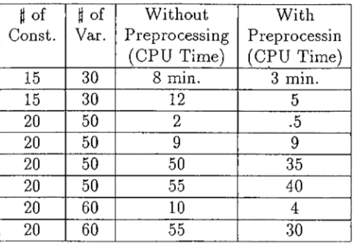
« o f Const. « of Var. Without Preprocessing (CPU Time) With Preprocessin (CPU Time) 15 30 8 min. 3 min. 15 30 12 20 50 .5 20 50 20 50 50 35 20 50 55 40 20 60 10 20 60 55 30

Table 1.1: Importance of Preprocessing

• Estimation of number of I ’s in feasible solutions, • Obligatory fixing of variables, e.t.c.

Any kind of enumeration method can be accelareted by these informations. The following computational results have been obtained with LINDO packages on a PC. In ’With Pre­ processing’ step, we append results of preprocessings to original problem such as objective function constraint, surrogate constraint, lower and upper bounds for the number of I ’s in any feasible solution of (BP). It can be seen that, except one problem, improvements are significant.

In Chapter 2, a combined heuristic method to generate feasible solutions is devoloped. Lagrange problem, surrogate constraint problem and some heuristics will be combined to find feasible solutions eflSciently in this algorithm. It will be shown that these solutions are reached in a very short time. And an algorithmic optimality test will be given. In Chapter 3, new bounding schemes for the number of I ’s in feasible solutions of (BP) is discussed. The calculation of these bounds takes polynomial number of iterations. In Chapter 4, a feasibility test for a special system of 3 linear inequalities with 0-1 variables is constructed. Then, this test is applied to improve bounds given in Chapter 3. In Chapter 5, a new algorithm to solve general (non-linear) 0-1 programming with linear objective function is discussed. Finally, some conclusions are made.

2. GENERATION OF FEASIBLE SOLUTIONS

There are several ways for the use of Lagrange Multipliers (LM) in mathematical pro­ gramming. Most of them is based on the paper, H.Everett [3]. The LM method is very simple, especially, in integer programming. A lot of papers are considering LM as a way to find a dual program for integer programming [22]. But LM is very useful algorithmic tool as well. It is used to decompose a large scale problem [6], or to reduce the number of variables [4]. The application of LM to generate feasible solutions and reduce the feasible region is discussed in [24].

In section 1, Lagrange problem, surrogate constraint problem and their relations are introduced [5,14]. In section 2, a combined heuristic to generate feasible solutions is de- voloped, and an optimality test will be discussed. Some test problems which are randomly generated are devoted to see that how these feasible solutions are good.

2.1

Background review

Relaxation methods in integer programming are very important. Two of them, Lagrange relaxation and surrogate constraint problem, are discussed here.

Consider (BP), its Lagrange Relaxation Problem (LRP) is given as L{\') = max a:g{o,i}n { ( c - A'A)a; + X'b'} where A' > 0 is a fixed vector, and optimal solution can be found as:

Xi = <

1 if Cj — X'a'j > 0 1 or 0 if Cj — X'a'j = 0 0 if Cj — X'a'j < 0 where a) is the column of A'.

Hence,

l ( y ) = Y ,\ c i - \ 'a 'i h + n '

(

.

,

)

where I7I+ = max {0,7} for any arbitrary real number 7.

L e m m a 2.1 [2] VA' > 0, (LRP) is an upper bound fo r (BP).

II.Everett [3] gave in 1963 the main theorem of LM method, and then Nemhauser and Ulman [20] generalized his result a bit more.

T h e o r e m 2.1 If x* solves problem (LRP) fo r a given A' > 0 and x ' is feasible in (BP) and

X f b - A ' x * ) = 0

then X * solves problem (BP).

The surrogate constraint problem [8] is defined as: max cx X'A'x < X'h'

X € {0,1) ” where A' > 0 is a fixed vector.

It can easily be seen that SP{X') is a relaxation of (B P).

L e m m a 2.2 L{X') is an upper bound o f SP(X').

(

.

.

)

(S P (\ '))

P r o o f : Let x* be an optimal solution of (LRP) for a given A'. Then L { y ) > c x + X ' ( b ' - A ' x ) V x G { 0 , l } " In addition,

Vx € 5 'P (A '), X ' { b ' - A 'x) > 0 . □

Although SP{X') is a good relaxation to (B P), computationally, solving (LRP) is much more easier than SP(X'), because SP(X') is a knapsack problem, therefore it is NP-hard.

2.2 A Combined Heuristic

The followings are some important properties of relaxation methods :

• solving relaxation problems are much more easier than original problem, these prob­ lems give an upper bound to original problem,

• if the optimal solution of these problems satisfying certain conditions is a feasible solution of the original problem, then it is optimal, too. E.g. in the case of (LRP), this extra condition is (2.1.2), as it can be seen from Theorem 2.1

Assume that a feasible solution, say, x° is known. Then we can add (BP) the following objective function constraint :

cx > Zo + I where Zo is the appropriate objective function value.

(2.2.1)

Then, it is enough to restrict ourselves to looking only for these feasible solutions, which have a better objective function value, i.e. the set of feasible solutions can be substituted by P = { x : A x < 6, X 6 { 0 ,1 } " } where and instead of A = b = A' —c b' -Zo — 1 P' = { x : A'x < 6', X G { 0 ,1 } " } .

It is obvious that if the optimal solution is better than the given feasible solution, it is in P.

If we have initially no feasible solution, then without loss of generality we can assume that cx > —1, i.e. it is no restriction. Later on, if a feasible solution is found, the objective function constraint can be updated. The set P is used instead of P', i.e. the problem is considered in the form

max cx X e P and (LRP) becomes, L{X) = max {(c — AA)x + A6} ( M B P ) ( M L R P ) where A = (A', A,ri+i) > 0.

In addition, S'P(A') turns out to be

max cx XAx < Xb X e {0,1}".

(,?P(A))

In [24], a new optimality criterion was given. It defines the optimality region of a feasible solution, say, x* generated by solving (MLRP), i.e.

arq max {(c — Ay4)a;} = x*. ®€{0,l}n

Then, the optimality region of x* is given as:

H {x \ X) = { x e {0,1} " I AAa:* - AAx > 0}

L em m a 2.3 [24] y4n optimal solution of the following system max cx X E P D H{x' ‘, A) is X*.

(

.

.

)

Lemma 2.3 is a good algorithmic tool for dividing feasible region in order to find optimal solution.

Let X* generated by (M LRP) for a given A 6 , be a feasible solution to (M BP). and let define

P ” = P n ii(a;*,A )^ (2.2..5)

where

H {x \ X y = { x e { 0 ,1} " 1 AAt* - AAx < 0}.

Since all coefficients are integer, therefore if A is an integer vector, then it is equivalent to H ( x \ x y = {x 6 { 0 ,1} " I XAx* - XAx < - 1}. (2.2.6)

T h e o r e m 2.2 Let x* be the point generated by (M LRP) fo r a given A > 0 and assume that it is a feasible solution o f (MBP). If there is a feasible solution having better objective function value, then it is in P ” .

P r o o f : By lemma 2.3, it is obvious. □

Surrogate constraint problem is used to generate binary vectors. The following lemma contains optimality criterion of S P {\) for (M BP).

L e m m a 2.4 Let x* be the optimal solution o f SP{ \) . If x* is in (MBP). then it is an optimal solution, too.

^ ^ (A ) is a hard-problem to solve. Therefore a greedy algorithm is used to find a feasible solution of SP{\). One can write SP{X) more explicitely as

max CjXj

AojXj < A,6,· a : j G { o , i } V i e J . To simplify the following steps, let us define

m 0 = a,-6,-i= l and aj = Xaj. (2.2.7)

Then, S P {\ ) becomes max i=i ajXj < ^ j=i X,· € {0.1}, Vi G J.

In addition, without loss of generality we may assume that there is an index p, such that <^j E 0 if i < p and aj > 0 ii j > p and furthermore

Cp+l/^p+l ^ C-p-\-2! ^ (^n· (2.2.8)

In this ordering, aj for some j can be equal to zero. But without losing this index ordering we can add a small quantity to denominators. Then, the following algorithm finds a feasible solution to SP{X).

A lg o rith m 1: A g re e d y a lg o rith m fo r SP {\) 1. b eg in 2. fo r j := 1to p d o 3. begin 4. Xj :== 1; 5. 15 : = 15 - aj] 6. end; 7. fo r j := p + 1 to n d o 8. if aj < 15 9. th en 10. begin 11. Xj : = 1; 12. 13·.- (5 - aj] 13. end; 14. end;

W ith this algorithm, we have x* solution to SP{X) for a given A > 0. Here the following question arises.

A r e th e re Lagrange m u ltip liers such th a t x* is th e o p tim a l solu tion o f the a p p r o p r ia te L agrange p r o b le m ?

If the answer is yes, then all of the properties of points generated by Lagrange multi­ pliers, e.g. the existence of the optimality region, can be preserved.

We will modify the result of [24], in such a way that A vector which is used to find x* is preserved here. In [24], A = 0.

Let’s extend (M BP) into

max z = cx

A : Ax < b p. : Ex < e

X e {0,1}

(2.2.9)

where E is the appropriate identity matrix and A and ¡x are respective Lagrange multi­ pliers. Let i > 0 be a real number. Consider the following (MLRP) :

maa;j;g{o,i}n {(c — t\A — ix)x}.

(

.

.

)

A r e th e re t and ¡x such th a t

arg max a:e{o,i}" {(c — tXA - i.i)x] = x ’ w h ere x* is th e any feasible solu tion o f S P {\ ) ?

Let k be defined as follows :

k = max = 1, and aj > 0}. (2.2.11)

If such k does not exists then there are two cases. The first one is that Vj aj < 0. It means that all components of a:* is 1 . Due to cost coefficient, it is the optimal solution if feasible. The second case is that 3p < n with ctp+i > 0. Then, \et k = p A 1 and we proceed as in the existence of k. So, choose

In addition. H = t = Ck/Xak Cj — tXaj ii j < k and Xj = 0 0 if not

(

.

.

)

L e m m a 2.5 For t and p chosen as above,

arg max a:€{o,i}n {(c - tXA - /x)x} = x*. 9

Cp+i/tAop+i > · · · > Ck-ilt\ak-i > 1 > Ck+i/tXak+i > ■■■> CnItXan. (2.2.14) Case 1: If i = k, then Ck — tXak — fj,k =

Case 2: if j > k and Xaj > 0, Cj — tXaj — ¡j.j = Cj — tXaj < 0,

Case 3: if j < k and Xj = 0, we have cj — tXaj — fXj = cj — tXaj — (cj — tXaj) = 0. Case 4 : if j < k and Xj = 1, then Cj — Xuj — m = Cj — Xaj > 0, due to (2.2.14).

□

Then, it follows that

cx* — cx > {tXA + ii)x* — (tXA + fj,)x, Wx G {0,1} " (2.2.15) In addition, the optimality region of x* is

7i(x * ,iA ,/z) = {a; G { 0 ,1 } " : (¿AA + /z)x* - (iAA + p)a: > 0} (2.2.16) Let us define

P ” = P f \ H { x ' ' , t X , n y (2.2.17)

where

H { x ‘ , tX, fiY = { x e { 0 , i y : {tXA + ij,)x^ - {tXA + fi)x < 0} (2.2.18) In the applications, instead of (2.2.18) the following is used

H { x y tX, nY = { x e { O A V ■■ {tXA + f i ) x , - { t X A + f i ) x < - e } (2.2.19) where e > 0 is a small number.

L em m a 2.6 If there exists a feasible solution better than x * , it is in P ''. O

These methods, i.e. solving the Lagrange problem or the surrogate constraint problem, does not guarantee that feasible solution will be found at the first run. If it is not found, then A vector will be modified. By these changes, the importance of constraints can be found. Importance means which constraints are much more difficult to satisfy. To collect this information, we can open an array such that each component of it corresponds the different constraint. Then if constraint i is infeasible for generated binary vector, then increase the vilolation number of this constraint by 1. The following modification of the Lagrange multiplier somehow reflect importance of the constraints.

Proof : If i = Ck/Xak·, then

Let X* be the generated binary vector and assume that it is not feasible to (MBP). Then, the following sets are introduced

and

Let us define

I{x*) — { i : aix* > bi}

J(x*)

=

:

Let r be a real number such that

¿2 — ^jbj·

s l + s 2 < tl + t 2

r > {t2- S2)/{Si - tl). Choose new Lagrange multipliers [8] as

vXk if A: G ^(x*) ^new _

Xk if not ( 2 .2 .20)

The idea behind that choice is as follows: Assume that all of the components of the vector A are positive and the vector x* is generated by A lg o r ith m 1. Then, x* satisfies constraint sets of SP{X). But,

^ Xidx* > Xibi ieiix") i€i[x*) and therefore

AjCjX < ^jbj.

j e J ( x * ) j ^ J { x * )

That kind of choice is a way to increase the weight of constraints which are not feasible. And the meaning of this kind of choice of r is described in the following lemma.

L em m a 2.7 I f r is chosen as in above and X is modified as in (2.2.20), then x* is not a feasible solution to 5'P(A” ®“').

r ♦ s i + s2 < r * tl + ¿2

Proof : If X* is a feasible solution, then

but this is a contradiction of

r > { t 2 - s2) / ( s l - i l ) . □

In [8], for a given A, SP(X) was solved optimally, and concentrated on the optimal solution of the (BP) because of Lemma 2.4. But, since S P {\ ) is a difficult problem, we are only concentrated on finding feasible solutions which are good and found in a short time.

Another heuristic to generate a feasible solution is as follows : Let x° be any start­ ing binary vector, e.g, choose x° as a binary vector generated by Lagrange problem or surrogate constraint problem. Then, let

n

5 (x °) = { i / € {0,1} " : = 1} 1=1

which is called the neighborhood set of x°. The following function, g measures infeasibility or objective function value, resp., of a binary vector x if it is infeasible or feasible, resp., where

cx if X is feasible

TaLi \^i - ■ if not

and the following set G contains all binary vectors in the neighborhood of x which are closer to be a feasible solution than previous ones;

g { x ) =

G{x) = { y e S{x) : g{y) > ^( x) }

Then we get the following heuristic method to generate feasible solutions.

(2.2.21) Algorithm 2 1. begin 2. k ■- 0; 3. Choose x°\ 4. while G(x^) 0 do 5. begin 6. Choose x*^+^ G G {x ’^)\ 7 . A::=fc + 1; 12

8. end; 9. end;

There are several ways to execute the choice described in Row 6. One possible way is to choose the first neighbor which better than a;*.

These heuristics can be combined. The following algorithm is a general scheme for this combination, and computational experiences show that it is very effective to find feasible solutions if there are any.

Algorithm 3: A combined heuristic 1. begin

2. A := A°

3. for A: := 1 to /

4. begin

5. Apply Algorithm ic G SP{\^) / * Binary Vector Generation * /

6. if G P 7. then 8. Put {2.2.1^) into P / * P := P D H {x'^ ,t\ ,p y */ 9. else 10. M o d i f y A vector as in (2.2.20); 11. end;

12. Apply Algorithm 2 with the starting point x ‘ ] 13. end;

Now, we will give an optimality test. The following statement is an immediate con­ sequence of the fact that the surrogate knapsack problem is a relaxation of the integer programming problem

i f S P {\) = 0, then P = ^.

For Algorithm 3, instead of arbitrary starting Lagrange multiplier, let us start with A° = (A ',0). Then, apply Algorithm 3 with the following rule :

RULE : Change the last component of A , which corresponds to objective function constraint, to positive quantity if and on ly if Algorithm 3 finds a feasible solution.

With this choice of vector A, the following theorem is valid: 13

T h e o r e m 2.3 With the. above R U L E , if S P {\) = 0 then, one o f the following statement is true: — i.e. original system is empty,

2) let Y be the set of feasible solutions obtained by the Algorithm 3. Then z = max cx.

xeY

P r o o f : If = 0, i.e, no feasible solution is found, it follows that S P{\) — SP{\'). It means iS'P(A') = 0. Therefore, P = 0, thus the problem is infeasible. On the other hand, if A,n+i > 0) then we have found a feasible solution. But, o P( A) = 0. Due to Lemma 7 and Algorithm’s property of adding constraint if we found a feasible solution, P” = 0. But, P ” is used whenever there is a feasible solution. This completes the proof. □

In this theorem, there are two test which are infeasibility test and optimality test.

T est : _n

rnin{0, Qfj} greater than (3 ? j= i

If the answer is yes and Am+i = 0, then original problem is infeasible, on the other hand, answer is yes and A„i+i > 0, then an optimal solution is found.

2.3

Computational results

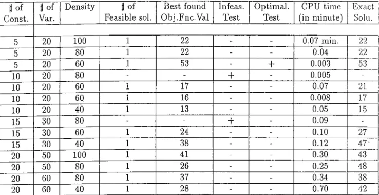
All problems are generated randorrily. To find exact value of problems, LINDO is used. Tableau 1 is for the comparison of generated feasible solution value and exact value.

Computational experiences show that, for some problems, feasible solutions that we found, are the optimal solution. If the problem is infeasible , it can be detected. For the third problem, algorithm concludes that optimal solution is found. In general, dif­ ference between exact values and objective values of feasible solutions are small, and in computational point of view, it runs in a short time.

H of Const. « o f Var. Density « of Feasible sol. Best found Obj.Fnc.Val Infeas. Test Optimal. Test CPU time (in minute) E.xact Solu. 5 20 100 1 22 - - 0.07 min. 22 1 5 ^ 20 ^ 80 1 22 - - 0.04 22 5 ^ 20 60 1 53 - + 0.003 53 10 20 80 - - + - 0.005 -10 20 60 1 17 - - 0.07 21 10 20 60 1 16 - 0.008 17 10 20 40 1 13 - - 0.05 15 15 30 80 - - + - 0.09 -15 30 60 1 24 - - 0.10 27 15 30 40 1 38 - - 0.12 47· 20 50 100 1 41 - 0.30 43 20 50 80 1 26 - - 0.25 48 20 60 80 1 37 - - 0.34 38 20 60 40 1 28 - - 0.70 42

Table 2.1; Result of Combined Heuristic

3. BOUNDING NUMBER OF I ’s IN FEASIBLE

SOLUTIONS

This part of the thesis refers to the set of the feasible solutions of 0-1 linear integer programming (M BP), i.e.

Ax < b

X G { 0 , 1 } ” (3.0J)

Generation of feasible solutions by heuristics are discussed in Chapter 2. This part of the thesis is to give bounds to the number of ones in feasible solutions [26,27,29].

In Section 1 of this chapter, two lower and upper bounds for the number of I ’s in any feasible solution are discussed. Section 2 contains a numerical example. Then, in Section

3, experimental analysis is provided.

3.1

Bounding Schemes

The detailed form of (3.0.1) is

n bi J=1 X j G { 0, 1} where / = {1, · · ■, m } and J = { l , · · · , n } . Wi e l Vi G J.

Define TTj to be a permutation over the set J for a given iGl in which the coefficients of constraint i are sorted in nondecreasing order i.e

^!7ri(l) — ^tV,'(2) ^ ^ ^17r,(n) (3.1.1)

There are three cases for any given constraint i e I 16

1. if bi > 0, then the origin 0 is a feasible solution for that particular constraint, 2. if ^ where N = {k : aik < 0 }, then there is no feasible solution for

constraint i, therefore (BP) is infeasible.

3· — ^'1 where N — {k : aik < 0}, then there is at least one feasible solution for constraint i.

Further developments requires some definitions.

D e fin itio n 3.1 pi{j) is the largest lower bound of the number o f 1 ’s that must he contained in any feasible solution of constraint i, if it exists with Xj = 1.

D e fin itio n 3.2 qi{j) is the smallest upper bound o f the maximal number of I ’s that can be contained in any feasible solution of constraint i, if it exists with xj = 1.

Assume that the indicies 7 and 0 defined by the following inequalities exist; Vi < 7, t 7 - 1 7 ^ ^ (3.1.2) k=l^k^j k=l^k:^j Vto > 0, w 0-{-l 9 ^iTTi(j) + ^ > CLiT^-[j) + <^17T,(/c) (3.1.3) k=\,k^j k=\,ki^j k=\,k^j

i.e. 7 .is the smallest and 0 is the greatest index i, such that t

<^t7r,(/c) + ^t7Tt(i) ^ ^i· k=ly k:ff:j

The shape o f function f { t ) = <3tir,(yt) is illustrated in Figure 1:

In figure 1

... represents a constraint i with positive coefficients, represents a constraint i with nonnegative coefficients,

--- represents a constraint i with negative, zero and positive coefficients. The possible values of p fij) and qfij) in (3.1.2) and (3.1.3) are

7 if a feasible solution with X7r,(j) = 1 exists

and

P.(7r.-(i)) =

;? .(7 r .(i)) =

n + 1 if not

9 if a feasible solution with = 1 exists — 1 if not

Hence, for a given constraint i, we have pi{j) = n + 1 i f f qfij) = - 1. Thus, if Vi e J, Vz G I. Pi{j) ^ n + 1, then p ,(i) < qfij).

The following statements are consequences of definitions; for any i €: I, li j < k then ^ i ’»(^t(^))· follows that for the same indices, <7i(7rt(i)) > g,(7r,(A·)).

The following figures are showing all of the possible cases of constraint i with x^d) = 1· In fact, these figures are conceptual figures, but they give a good idea about pfiirfij)) and

values.

f i r t /N - · « r I 9 I 9 > / • I / I t \ / i

Figure 2: Possible values of pi{TTi{j)) and qi{'Ki{j)).

Let l{j) be the number of I ’s which must -be contained in any feasible solution of (3.0.1) if such exists with Xj = 1. Then

Vj e J, p (j) = max i pi{j) < l{j). Hence, for any feasible solution x with Xj = 1, we have

(3.1.4)

pU) < (3.1.5)

k=l

Let u{j ) he the maximal number of I ’s that can be contained in any feasible solution vs that

Vi e J, u( j ) < q{j) = min .· qi{j). (3.1.6)

X with Xj = 1. It follows that

and

Y ^ X k < q{j).

19

(3.1.7)

Further on we use only numbers p{ j ) and q{j), instead of l{j) and u{ j ) respectively. Consider the index set

J{ x) = { j : Xj = 1} (3.1.8)

where a; is a feasible solution. It follows that |J(a:)| is the number of I ’s in a:, i.e

n

' ^ X j = l·^(2:)|■ i=i

L e m m a 3.1 For any given feasible solution x ^ 0 to (3.0.1),

y j e J { x ) , p ( i ) < |J(a:)|.

P r o o f : By definition of p (j), it is obvious. □

The next theorem is the generalization of Lemma 3.1. It gives a lower bound for the number of I ’s in any given feasible solution. We will call it as a trivial lower bound in the sense that only definition of p{ j ) is used.

T h e o r e m 3.1 Let x ^ 0 be any feasible solution. Then,

n

> min ,■ p (;). (3.1.9)

J=1

P r o o f : Let P be the set of feasible solutions of (M BP) By lemma 3.1, we have that Va: € P \ {0 }, Vi G J{ x) , p{j) < |J(a:)|.

Since I J(a;)| = h follows that n

min j p{ j ) < ^ X j , V.a: 6 P \ {0 }. □ i=i

The next lemma is for upper bound which is also called trivial.

L em m a 3.2 For any feasible solution x,

q{j)>\J{x)\

if jeJix).

P r o o f : The statement follows immediately from the definition of ? ( i ) ’s. □ 20

n

' ^ X j < max j q{j). j=i

Theorem 3.2 For any feasible solution to (MBP),

(3.1.10)

P r o o f : The proof is similar to the proof of the previous theorem. □

Now, we will give second lower and upper bounds for any feasible solution. These bounds are at least as good as obtained from Theorem 3.1 and Theorem 3.2.

Let’s define Li as the set of variables which can be contained with Vcilue 1 in at least one feasible solution if it exists with at most I I ’s. In other words,

v /e { l,··■,..),

i, = {; : i(i) < (}

It follows from (3.1.6) that,

Li C { j : p { j ) < l } = T,.

It is obvious that

C T2 C . . . c

T h e o r e m 3.3 For any feasible solution, x ^ Q, we have

n ^ X j > UJx i=l where (3.1.11) (jj\ — m in{/ : |T/| > I, I > 1}.

P r o o f : Let us consider a feasible solution x with exactly I I ’s in it. Then Vj E J{x), p{ j ) < 1. Hence, J{x) C T/. Now, I — |J(a:)l < |T/| and thus the statement

follows. □

For a given / € { I , ·' ‘ define Ui such that it contains only variables which could be with value 1 in a feasible solution which solution contains at least I I ’s, i.e.

It follows from (3.1.6) that

It is obvious that

U l = { j : u U ) > / )

Ui 5 0 : iO') > l ) = S,.

Si 5 «2 3 ■ ■ ■ 3

n

< L02 j=l

Theorem 3.4 For any feasible solution x , we have

where

u>2 — m ax{/ : \Si\ > I, I > 1}.

(3.1.12)

P r o o f : The proof is similar to the proof of the last theorem. □

The following two algorithms are constructed to determine the values u>i and u>2.

A lg o r ith m a>i 1. b eg in 2. count \= —1; 3. / := 0; 4. w h ile count < I d o 5. b eg in 6. / : = / + !; 7. count := 0; 8. fo r j := 1 to n d o 9. _{if V{i) < ^} 10. then 11. count = count 12. end; 13. LOl = 1] 14. end; 1. b e g in 2. count := 0; 3. 1 n \ 4. w h ile count < I d o 5. b e g in Algorithm CU2 22

6. 7. count := 0; 8. fo r j := 1 to n d o 9. _{i f} q { j ) > ^ 10. th en 11. count ·.— count 12. en d; 13. CU2 := 1 14. end;

The following theorems and corrolaries are the consequences of the previous theorems and lemmas.

T h e o r e m 3.5 I f uji > u>2, then (MBP) is infeasible. □

T h e o r e m 3.6 I f p{ j ) = n then for any feasible solution x, xj = 0. □

C o r r o la r y 3.1 { j : q{j) = - 1 } = { j : p{j) = n + 1}. □

C o r r o la r y 3.2 If there exists an index j with q[j) = n, then e is a feasible solution,xohere e is all 1 vector.

P r o o f : By definition of q{j), Vi G / , qi{j) = n, i.e. Vz G / , the vector consisting of n I ’s is feasible. □

C o r r o la r y 3.3 If fo r an index j, q[j) < p{j), thenxj = 0 in any feasible solution. □

3.2

A n Example

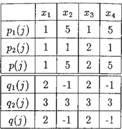
Consider the following system of linear inequalities:

—3xi + 4x2 — 2x3 + 5x4 < —2 2xi — X2 + 4x3 — 2x4 < 2

x. G {0 ,1 }, z = 1 ,2 ,3 ,4 23

a;i X2 X3 X4 P i(i) 1 5 1 5 P2{j) 1 1 2 1 pU) 1 5 2 5 9 i(i) 2 -1 2 -1 92 (i) 3 3 3 3 9 (i) 2 -1 2 -1

Tableau 1: Results of computations

If we analyze Tableau 1, we can say that X2 = X4 = 0 due to Theorem 3.6. Moreover, cui = m inj p{j) = 1 and u>2 = maxj q{j) = 2. Therefore, by Theorem 3.3 and 3.4, we have

. Hence,

1 < j=i

\ < X\ -r X:i < 2

If we rewrite P with X2 = X4 = 0, nothing is lost in the sense of feasible points. Then, new system is given by :

—3xi — 2x3 < —2 2xi T 4x3 ^ 2 X\) X3 € {0,1}

Then if the algorithm is applied again, then the following results are obtained.

X l _{a ; 3} P i(i) 1 1 P2U) 1 5 pU) 1 5 9 i(i) 2 2 9 2 ( i ) 1 - 1 9 (;) 1 - 1

Tableau 2 : Result of second iteration of algorithm

Hence, X3 = 0. The final result is that, the only feasible solution is (1,0,0,0). 24

3.3

Experimental Results

In this section, computational experiences are discussed. Tableau in Chapter 4 provides informations about coi, cu2, exact lower and upper bounds. All of these problems are generated randomly. To find exact lower and upper bounds for the number of I ’s that must be satisfied by any feasible solutions other than 0, LINDO package is used.

The calculation of uji and u>2 takes polynomial number of iterations, p and q vectors can be used in any enumeration algorithm for bounding number of I ’s in an}' subset of feasible solutions within a verv short time.

4. IMPROVEMENTS ON BOUNDS

This part of the thesis is devoted to improve bounds discussed in the previous chapter. In Section 1 of this chapter, a feasibility test for 3Tinear constraints of 0-1 variables is given. Then, in Section 2, this test, for a special system, is going to be applied for sharpening the upper bound and improving the lower bound. One of these constraints is the objective function constraint, the second one is the surrogate constraint with special choice of Lagrange multipliers, and the third one is the constraint of the number of I ’s that can be contained in some feasible solution. The last constraint has varying right hand side, say a;, such that co G [101^0^2]· In Section 3, computational experiences will be discussed. Finally, some conclusions are obtained.

4.1

A Feasibility Test

Let us consider the set of binary vectors

n n n

P{uj) = {x e { 0 ,1 } " : Y^dj Xj > T], < p, ^ X j = w}.

j = l j - l j = l

where the two inequalities are consequences of the constraints of the (M BP) problem. If P{u>) is empty, then the (M BP) problem has no feasible solution with exactly lo I ’s.

An easy test to check this is developed here. First of all, some preliminaries are required. Let us define

n n

P

{

)

u}.

}=1 j = l

It is obvious that P {oj) C Po(u>). The following lemma will be called ’main lemma’ .

L em m a 4.1 I f 3 y G Po{^) with djyj > t], then P {uj) 7^ 0. □ 26

Let us consider the following 0-1 Integer Programming problem:

Su) — max ^j^'j

X e Po{<^) (4.1.1)

The following lemma is equivalent to Lemma 4.1 in the sense that if one of them has a positive result, so has the other one. Positive result means P{u>) ^ 0.

Lemma 4.2 6^^ > r] iff P(u>) ^ 0 . □

Thus

P(oj) = 0 i f f < rj.

But (4.1.1) is a diffucult problem. Let us consider the LP relaxation of P{u>) and Po{>^) as P'{oj) and i.e.

n n n P'{oj) = { x : ' ^ d j X j > T j , ' ^ a j X j < p, ' ^ X j = cu, 0 < a; < e} j=l j=l j=l a.nd n n P'o{>^) = < p, 0 < .T < e} i=i j=\

where e is the all 1 vector.

It is clear that P{uj) C P'(cu) and Pq C Pffu>). Then, instead of (4.1.1), the following LP problem can be solved :

61 = max djXj

x e P'(cu)

(4.1.2)

(4.1.2) is an easy problem to solve. Its constraint set has special structure and upper bounding version of simplex method can be applied as a solution scheme very efficiently. Then, the following lemma arises :

L e m m a 4.3 I f 8'^ < t], then P{u)) = 0.

P r o o f : If (5^ < 7], P'{u>) = 0, but P(tu) C P'{u)). □

Thus, a feasibility test is obtained for a system of 3 linear inequalities with 0-1 vari­ ables.

4.2

Application of Test

In Chapter 2, a combined heuristic which generate feasible solutions to (M BP) have been developed.

The following problem is identical to (M BP) :

(4.2.1) // > 0 are problem : max z = cx A : A x < b /.I : E x < e x G { 0 ,1 } ’^

where E is the appropriate identity matrix, e is the all 1 vector, A > 0, and appropriate Lagrange multipliers. Consider the following surrogate constraint

SP{X,iJ,) : max Z = cx (AA + fi)x < \b + /j.e

X e { 0 ,1 } ” . Let x° be a feasible solution of S P { X ,0) i.e.,

max Z = cx XAx < Xb X G { 0 ,1 } ”

and assume that x° is also a feasible solution of (MBP). Then, there exists t and /i (2.2.12-13) such that

argmax { { c — tXA — ii)x : a: 6 {0 ,1 }” } = x,.o in other words

max { { c — tXA — ix)x] = {c — tXA — f.i)x°. Then, we have the following surrogate constraint :

{tXA -f fi)x < tXb -1- ¡.LC (4.2.2)

It can be seen that Vx G P, x satisfies (4.2.2) . In addition, optimality region of x° is defined as

{tXA -f fi)x° — {tXA + [Pjx > 0.

It can be seen that if x° is not an optimal solution of (M BP), then it must satisfy

{tXA + ¡j,)x° — (tXA + n) x < —e (4.2.3)

where e > 0 is the appropriate small number. The objective function constraint with this feasible solution, is defined as

cx > Zo + I (4.2.4)

where Zo = cx°.

If there is a feasible solution having better objective function value then Zo, it must satisfy (4.2.4). Furthermore, assume that we have an upper (lower) bound, say, lo, for the

number of I ’s in feasible solutions of P is known, i.e.

< ( > V · j=i

Consider the following sets of binary vectors defined by linear inequalities :

(4.2.5)

P i ( u ) ) = { a : G {0, !}"■ : c x > Z o + l, (tXA + n) x < tXb + jj,e, = (4.2.6)

J = 1

= {x e {0 ,1 }" : cx > Zo + 1, {tXA + fi)x° - {tXA + fi)x < - e , ^ xj = u;](4.2.7) J = 1

P\o{p) = {a: G {0, !}"■ : {tXA + n)x < tXb + ^e, ^ Xj = a;} (4.2.8) i=i

and

P2o{(^) = {a: G {0 ,1 } ” : {tXA + n)x° - (tXA + fj,)x < - e , ^ xj = a;} (4.2.9) J = 1

L e m m a 4 A If Pi(u>) = 0, or P2{u>) = 0, then in any feasible solution with cx > Zo we have Xj < w (X^”=i > ac).

P r o o f : Since we assumed that 3 x* such that it is feasible to P and ex" > Zo + 1· D Let us modif}' problem (4.1.2) for these new constraints as

Si = max

x e P /o H 29

= max YTo=\

(4.2.11)

where Plo(<^) and P^oi^)^ resp., are the LP relaxations of Pxo((^) and Pio(o;), resp.

Then, the following algorithm gives sharpened upper bound of the number of I ’s in any feasible solution.

A lg o r ith m : S h arpen in g 1. b e g in 2. / := true·, 3. to := u>2] 4. w h ile / do 5. if SI, (5") < Zo + 1 6. th en 7. u> u> — 1 8. else 9. / := false·, 10. end;

As a result of this algorithm and Lemma 4.4, the following corrolary is valid. It is a test for a given arbitrary u> that no need to search for larger lo values.

In above algorithm, if we choose u> as u>i at step 3 and cu = iu + 1 at step 7, lower bound cji can be improved.

4.3

Computational results

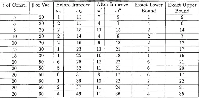
All of the problems are generated randomly.. ’Before Improve.’ column values are results of the algorithm that are found in Chapter 3. Last two columns is for the exact lower and upper bounds of some problems calculated by LINDO. Computational experiences shows that improvement are significant. Objective function and surrogate constraint are very effective over the upper bound, lo^. Diference between exact upper bound and uj" are,

in general, very small. Only one problem has diference value as 4. Surrogate constraint, upto finding feasible solution to (M BP), collects aggregate information about the problem.

D of Const. (t of Var. Bef CUi ore Improve. CJ2 Aft . cu' er Improve. co" Exact Lower Bound Exact Upper Bound 5 20 1 11 7 9 1 9 5 20 2 11 4 7 4 6 5 20 2 15 11 15 2 14 10 20 2 14 4 8 2 7 10 20 2 16 6 13 2 12 15 30 1 23 11 21 1 17 15 30 1 25 10 18 1 16 20 50 6 25 12 22 6 21 20 50 5 32 11 21 6 20 20 50 6 31 8 17 . 6 17 20 60 1 36 10 22 2 22 20 60 2 37 11 24 3 21 20 60 4 49 11 36 4 35

Table 4.1: Lower and Upper Bounds

Special choice of Lagrange Multipliers, until generation of feasible solution, makes this information more compact.

Due to special structure of the constarint set of (4.2.10), computation of 8'^ consumes very low CPU time, and above algorithm runs at most u>2 — U times in which U is the exact upper bound.

5. A NEW ALGORITHM TO SOLVE GENERAL

(non-linear) 0-1 PROGRAMMING

In this chapter, a new algorithm to solve general 0-1 programming problems with linear objective function is developed. Furthermore, this algorithm is adopted to solve linear 0-1 programming problems. The solution of the original problem, is equivalent with the solution of a sequence of set packing problems with special constraint sets. The solution of these set packing problems is equivalent with the ordering of the binary vectors according to their objective function value. An algorithm is developed to generate this order in a dynamic way. The main tool of the algorithm is a tree which represents the desired order of the generated binary vectors.

General 0-1 programming problem with linear objective function can be stated as: max cx

x e S C {0 ,1 }" ( G B P )

where c G and without loss of generality it is assumed in the whole chapter that Cl > C2 > · · · > Cn > 0. (5.0.1) It is well-known that the above problem (GBP) is a hard problem to solve if S has no special properties. If 5 is a set of linear inequalities with 0-1 variables, then it is (BP).

In [11] and [17], the following scheme is applied to solve the problem :

li ¡3i = e E. S , then it is optimal where e is the all 1 vector. If e ^ S', then the optimal solution of (G BP), if it exists, must satisfy the following inequality

n

X j < n — \.

i=l

/?2i =

Let us consider the following problem : Z-i — max cx

(5.0.2) X e {0 ,1 }"

and assume that its optimal solution is /32- Then, it is obvious that if /?2 6 S, then it is an optimal solution of (GBP). It can be seen that

1 i f j e {1,...,72 - 1} 0 i / i = n

Now assume that ^2 ^ S, it follows that optimal solution of original problem must satisf}^

n

X j < n —

1

< 7^26 — 1

X e (0,1)"

If we continue this procedure, the following generalization is obtained.

Assume that /?i = e,y02, ···, have been generated so far and none of them was feasible to (G B P). Then, solve the following set packing problem :

Zk+i = max cx

x e P k = { a ; G { 0 , l } " : - 1, / = 1, .·., ^^} { S P P ) and assume that the optimal solution of { SPP) is

L em m a 5.1 Assume that /3i,...,Pk ^ S. Then S C P^.

P r o o f: Let us assume that y G {0 ,1 } " , y ^ {^x, ...,^/.}, but y ^ Pk- Consider the following index r such that

r = min {I : ¡3iy > 0ie — l } . It is obvious that r > 2. Otherwise, ?■ = 1, y = ^1. It follows that

fSry = Pre i.e.,

y > ^T-Hence, it follows from (5.0.1) that

cy >

c^r-This is a contradiction to optimal property of /?r, because y G P r-i· 33

Lemma 5.2 (SPP) is a relaxation o f (G B P ).

P r o o f: By previous lemma, Va; G -S', a; G Pr-. □

T h e o r e m 5.1 Let k be the minimal index of iterations, such that ^ -S'. Then it is optimal to (GBP).

P r o o f : It follows from previous lemmas. □

5.1

Boros’ Idea

It was Boros [1] who made the following observation in 1985. This solution scheme of sequence of set packing problems is equivalent to the ordering of the binaiy vectors in decreasing values of the objective function value. As it is stated in Lemma 1, the constraint set of the current set packing problem excludes only the points, generated so far. Therefore the optimal solution of next set packing problem is the best nongenerated binary vector.

Let L be the list that obeys above property. Then, the first feasible element of L is an optimal solution.

E x a m p le : let c be the following decreasing vector : c = (6 ,4 ,3 ,3 ) Then, L contains

T = {(1,1,1,1), (1,1,1,0), (1,1,0,1), (1,0,1,1), (0,1,1,1). (1,1, 0,0),

(1 ,0 ,1 ,0 ),....,(0 ,0 ,0 ,0 )}.

5.2

The Tree Representation of the Ordering of the Binary

Vectors

In this section the following problem is discussed ;

H ow can a seq u en ce o f th e b in a ry v e cto rs b e gen era ted in w h ich th e values o f th e lin ear fo rm cx are in a d e cre a sin g o rd e r ?

First of all, the subproblem is solved, where only the vectors having exactly in k components the value 1, i.e.

j=i

(5.2.1)

are ordered. Let u and v be two binary vectors satisfying (5.2.1). Let {¿i, *2, and resp., the set of indices of the I ’s in the vector u and v, resp. It follows immediately from (5.0.1) that if

^ jpt P — ' ' ' 1 k (5.2.2)

then cu > cv.

D e fin itio n 5.1 Let {¿i, ...,u } be the set of indices o f I ’s in the binary vector u. Assume that fo r some index p the inequality

ip “h 1 ^p+i

holds, where ik+i = n + 1. Then an immediate successor of u is the vector u', if /

j 7^ ”1" 1 = < 0 i f j = ip

I 1 i f j = ip + 1

Any vector V satisfying (5.2.2) is a successor of u.

It is obvious from previous remarks, that u is an immediate successor of u, then cu > cu .

T h e o r e m 5.2 Let {ii,...,U -} and { j i , ■■■■¡jk}, resp., be the sets o f indices of the I ’s in the binary vectors u and v, resp. Assume that (5.2.2) holds. Then there is a-sequence of binary vectors

Wo = U, W i , . . . , W i — V, such that wi is an immediate successor o f wi-\ (/ = 1, ...,t).

(5.2..3)

P r o o f : Assume that u ^ v, otherwise t — 0 and the statement holds. Let p = m ax {q : i, <

Hence = 0, otherwise

*p + 1 = ip+i ^ jp < ip+i 35

and this contradicts the maximal property of p. Let

{

i / i 7^ ip,

1

0 i / i = ip

1 i / i = ip + 1 Then the set of the indices of I ’s in Wi is

— '{il,···, ^p—1 j^pT 1,···,^/:}· It is obvious that

ill < ji, I — 1,

Then either wi — v, or the process can be repeated for wi. □

It is trivial that all of the binary vectors containing exactly k I ’s is the successor of the vector x, where Xi = ... = a:^ = 1, Xk+i = .·· = a;„ = 0. Therefore all of these vectors can be enumerated with the following algorithm, where L is the list of binaiy vectors to be enumerated. Algorithm 4 1. B egin 2. L : = {x = (1, ...,1,0, ....,0 )}; 3. w h ile L 0 do 4. b e g in 5. choose u ^ L] 6. L (L U {v : V is an immediate successor o f u }) 7. end; 8. en d

Without any deeper organization this algorithm will work unnecessarily too much, because the sequence (5.2.3) is not unique, i.e. a binary vector can be generated several times as the immediate successor of different vectors. This phenomena is illustrated with the following example. Let k = 2, n = A. Then Algorithm 4 starts from the point X = (1 ,1 ,0 ,0 ). In the first iteration it has only one immediate successor, which is Ui = (1 ,0 ,1 ,0 ). The immediate successor of ui are «2 = (0 ,1 ,1 ,0 ), and 113 = (1 ,0 ,0 ,1 ). The only immediate successor of U2 is 114 = (0 ,1 ,0 ,1 ) which is at the same time immediate successor of «3, too. To avoid this disadvantageous effect the following ordering of binary vectors is introduced.

D e fin itio n 5.2 The vector u is ’greater’ than v, denoted u t> v if either

• cu > cv or

• cu = cv and u is lexicographically greater than v which is denoted by u y v.

It is obvious that any two distinct vectors are comparable by this ordering, i.e. in any set of binary vectors there is a unique maximal element in this ordering. Thus the choice of the vector u in the 5-th row of Algorithm 4 can be executed in the following way

5' u := ?nax ^ {u E X}.

It follows from (5.0.1), that if u' is an immediate successor of u, then u t> id. Hence the following statement is obtained.

L em m a 5.3 If in Algorithm Jf. the choice of the vector u is done according to 5 ’, then, no vector can be chosen twice.

P r o o f : Assume that the vector u was chosen in iteration t. Then it was the maximal vector in ordering > which was contained in L and it was substituted by a set of smaller vectors. If it returned to L then at least one vector had to be substituted by a greater vector, which is impossible. □

Hence the following algorithm is obtained to enumerate all of the binary vectors. The vector 6j is the j-th unit vector.

Algorithm 5 1. B e g in 2· L : = : k = l,...,n }·, 3. w h ile T yi 0 do 4. b e g in 5. u := max^ {v € L }; 6. L := (L U {v : V is an immediate successor o f u }) \ {u ); 7. end; 37

8 . e n d

T h e o r e m 5.3 All o f the binary vectors are chosen in row 5 o f Algorithm 5 exactly once.

P r o o f : It follows from lemma 5.3 that it is enough to prove that all of the points are chosen at least once. Assume that the vector v containing exactly k I ’s is not chosen. Let us consider a sequence (5.2.3) from the point to v. Without loss of generality we may assume that in this sequence only v was not chosen. Then wt — v an immediate successor of which was chosen in an iteration. When in row 5 xi was Wt entered to L according to row 6. If u is in L and v has been never chosen then L has become never empty. Thus it follows from Lemma 5.3 that it should be infinite many binary vectors being greater in the ordering > than v, which is a contradiction. □

For the sake of convenient handling of the list L it is organized as a rooted tree. The root contains always the greatest point. All of the nodes of the tree, except the root, can have two children, a left and a right one. The root has only a left child. All of the binary vectors of the left (right) subtree of a node are less (greater) than that of v according to the relation t>. Thus it is very easy to find the appropriate position of a newly generated binary vector in the tree. This is done by Algorithm 6.

Algorithm 6

1. b e g in

2. {* Let L be the current tree *)

3. (* S := Set o f all immediate successor o f x *) 4. X := Binary vector in the root]

5. w h ile 5 7^ 0 d o 6. b e g in 7. y e S] 8. 2: := cy] 9. p := root''.left] 10. / := true]

11. w h ile p 7^ nil and f d o

12. b e g in 13. Temp := p] 14. if z > p^.obfv 15. th en p := p^.rightnode 16. else if z < p^.obfv 17. then p := p^.leftnode 18. else if y >- p^.BVector] 19. th en p := p^.rightnode·, 20. else if p^.B Vector >>- y 21. th en p^ .leftiiode 22. else 23. b egin 24. / := false·, 25. S : = S - { y } · , 26. end; 27. end; 28. i f f 29. th en 30. begin ; 31. 5 : = S \ W ; 32. if z > Temp^.obfv 33. th en Temp'^.rightnode := y 34. else if 2T < Temp^.obfv 35. then Temp'^.leftnode ·.— y

36. else if Tem p^.BVector >- y

37. th en Temp'^.leftnode :■

3 8 .

3 9 . e n d ;

4 0 . e n d ;

else Temp'^.rightnode := y;

In the row 6 of Algorithm 5, the point contained in the root is omitted from the tree. Therefore a method is needed to find the point, which must go into the root, i.e. the maximal binary vector in the tree. But, notice that this is always the most right point of the (left) subtree of the root.

As a implementation of the above algorithm, let Lk be the current tree at step k, and assume that Xk, binary vector in the root, is not feasible to (GBP), otherwise it is optimal, and S is the set of immediate successor of Xk- Then

Lk+i := Lk U S \{a;A;} (5.2.4)

E x a m p le : Assume that = 6, c = (7 ,5 ,4 ,3 , 2,1) and the current tree Lk consists of the following binary vectors

X k = ( 1 , 0 , 1 , 0 , 1 , 0 ) y i = ( l , 0 , l , 0 , 0 , 0 )

y2 = (1,1,0,0,0,0)

ya = (0,1,0,1,1,0)

y4 = ( l , 0 , 0 , 0 , 0 , 0 ) and the tree representation is

then immediate successor of Xk are

u = ( 0 , l , l , 0 , l , 0 )

u = ( l , 0 , l , 0 , 0 , l ) 40

u; = (1 ,0 ,0 ,1 ,1 ,0 ) then tree becomes

r- -'L

V X

Then point j/2 goes into the root and the shape of tree is

V

In Chapter 3 and 4, the lower and upper bounds were given for the number of I ’s in any feasible solution of 0-1 integer programming. If (GBP) is assumed to be 0-1 linear integer programming, these bounds can be used to make improvements in the algorithm.

5.3

A n Example

Consider the following problem

max 2xi -f X2 + 3xa + 4x4 3xi + 2x2 + + 4x4 < 3

then

2xi 4x2 "t" 2x3 4" 3x4 ^ 6 Xi, X2, X3, X4 G {0, 1}.

C4 > C3 > Cl > C2

(P)

Therefore, index set used to generate immediate successors of binary vector in the root is (4,3,1,2). So, for the initial tree (To)» the following binary vectors is used.

{ (1,1,1 ,1 ), (1 ,0 ,1 ,1 ), (0 ,0 ,1 ,1 ), ( 0 ,0 ,0 ,! ) } = {x o ,x i,X2,X3} cind tree becomes

Xo

(1,1,1,1) ^ P then tree turns out to be

Binary vector in the root is (1 ,0 ,1 ,1 ) ^ P and its ordering with respect to objective function value is (1,1,1,0). Immediate successor of it in this ordering is (1 ,1 ,0 ,1 ) and corresponding binary vector is X4 = (0 ,1 ,1 ,1 ). If we append it to the current tree, then tree becomes

Xv

L,

The binary vector in the root is (0 ,1 ,1 ,1 ) ^ P and its ordering is (1,1,0,1). Then the immediate successor of (1,1,0,1) is (1,0,1,1) and corresponding binary vector is

X5 = ( 1 ,1,0,1). If it is put in tree, tree becomes

The following iterations is similar and these are shown without explanations

L, L 5 K1 u .. ■'> ■T

8

8

8

Now, we shall use informations, the bounds for the number of I ’s , found in Chapter 3 and 4. The followings are the p and q vectors (see. Chapter 3)

p = ( l , 1,1,5), g = ( 2 , 2 , 2 , - l ) It follows that a;4 = 0 by Theorem 3.6. Then S (x4 = 0) is

3a;i + 2x2 + xa < 3 2a:i + 4x2 + 2xa < 6

so if we calculate p and q vectors, then p = (1 ,1 ,1 ), q = (2 ,2 ,2 ). Then, no need to search for the subproblems having total number of I ’s greater than two I ’s. In addition,