SI:M:PLiX.mBLHÄÜ SÄSSG
РВШ ІШ О Ш
. ' ' Ш , :ÂÀilMSJlXAIt'S . ДіЗОЕЛГШіІ ' .
. ' ^
f.ii J'ιΓ’ζ -■¡2ı,-·. ... S :U 3 J v n T T £ D ’ T O T N E 0 £ Р Д й Т ? ^ £ Ж , O r Ifc& U S T ^^ . Áu'“;D· ■ ^0 İ!E:’- C£-S' D'·^ '¿¿'^ :.XS1îT .’•Jы ιί . І ч ^ α . й - : ''· ·ν · » . V « . · · Ѵ Ч м Л 4 L ’ W··—*', W"·'·.. ■· ^ '» ·«»! я—1, ,■ і· щ»ш » '■«■■» λ :' Ч $ -Г: ■!,>* » · . V"*т:ьг‘? ;р ,;^.п :н іАѵ ·-«· W н ««Я· 'H.··. ·<λΤ* i .« І* í w áwW '■- « Vt·» ІІГ.ГХ"·?-· ’-Г -С^:‘С '-Ζ· ,··*■·.·■“ ' ч *;^-g* ч .. ·*■ U; ¡ ·Ζκ· 'фм^ '«Μ» •■^ V ·; !^ц· U« . ‘*Α .·*** ·.'"i-İî ·£;■ !*Ч.* ·'* 'V!^·'' ,i*~-^}p^. .!іц*.і}·. * •.|· -im :"ν; İÇ ** i* . .
/9 9 0
. /· .(♦ j Λ . !ti _ n * .; ■
SIMPLEX TABLEAU BASED APPROXIMATE PROJECTION
IN
KARMARKAR’S ALGORITHM
A T H E S IS S U B M I T T E D T O T H E D E P A R T M E N T O F I N D U S T R I A L E N G IN E E R IN G A N D T H E I N S T I T U T E O F E N G IN E E R IN G A N D S C IE N C E S O F B IL K E N T U N I V E R S IT Y IN P A R T IA L F U L F IL L M E N T O F T H E R E Q U I R E M E N T S F O R T H E D E G R E E O F M A S T E R O F S C IE N C EBy
Yaviiz Giinalay
September, 1990
T
i 0
I certify that I have read this thesis and that in my opinion it is fully adequate, in scope and in quality, as a thejjs for theiaep;ree of Master of Science.
Assoc. Prof. Mus rincipal Advisor)
I certify that I have read this thesis and that in my opinion it is fully adequate, in scope and in quality, as a thesis for the degree of Master of Science.
Prof. Halim Doğrusöz
I certify that I have read this thesis and that in my opinion it is fully adequate, in scope and in quality, as a thesis for the degree of Master of Science.
Assoc. Prof. @gman Oğuz
I certify that I have read this thesis and that in my opinion it is fully adequate, in scope and in quality, as a thesis for the degree of Master of Science.
Assoc. Prof. Bela Vizvari
Approved for the Institute of Engineering and Sciences:
/1 1 A
Prof. MehmetiBciray
Director of Institute of Engineering and Sciences
ABSTRACT
SIMPLEX TABLEAU BASED APPROXIMATE PROJECTION
IN
KARMARKAR’S ALGORITHM
Yavuz Giinalay
M.S. in Industrial Engineering
Supervisor: Assoc. Prof. Mustafa Akgiil
September, 1990
In this thesis, our main concern is to develop a new implementation of Karmarkar’s LP Algorithm and compare it with the standard version. In the implementation, the “Simplex Tableau” information is used in the basic step of the algorithm, the projection. Instead of constructing the whole projection matrix, some of the orthogonal feasible directions are obtained by using the Simplex Tableau and to give an idea of its effectiveness, this approximation scheme is compared with the standard implementation of Karmarkar’s Algorithm, by D. Gay. The Simplex Tableau is also used to calculate a basic feasible solution at any iteration with a very modest cost.
K ey w o rd s: Karmarkar’s LP Algorithm, Simplex Tableau.
ÖZET
KARMARKAR’IN ALGORİTHMASINDA SIMPLEX TABLOYA
BAĞLI YAKLAŞIK İZ DÜŞÜM UYGULAMASI
Yavuz Günalay
Endüstri Mühendisliği Bölümü Yüksek Lisans
Tez Yöneticisi: Doç. Mustafa Akgül
Eylül, 1990
Bu çalışmada, Karmarkar’ın Doğrusal Programlama Algoritmasının yeni bir uygulaması geliştirilmiş ve bu uygulama standart algoritma ile karşılaştırılmıştır. Uygulamadaki yenilik “Simplex Tablo” bilgisin den yararlanılmasıdır. Her iterasyonda projeksiyon matriksinin hesaplanması yerine “feasible” yönler Simplex Tablodan yararlanılarak bulunmuş ve bu yönlerin bir bölümü kullanılarak değer vektörünün yaklaşık iz düşümü hesaplanmıştır. Ayrıca, herhangi bir iterasyonda Simplex Tablo kullanılarak bir köşe noktasının ziyaret edilmesi çok az bir extra çaba gerektirmektedir.
A n a lıta r k elim eler: Karmarkarhn Algoritması, Simplex Tablo.
ACKNOWLEDGEMENT
I would like to thank to Assoc. Prof. Mustafa Akgiil for his supervision, guidance, suggestions, and patience throughout the development of this thesis. I am grateful to Prof. Halim Doğrusöz, Assoc. Prof. Osman Oğuz and Asst. Prof. Bela Vizvari for their valuable comments.
My sincere thanks are due to all of my close friends, both from Bilkent and outside, even from US, for their valuable remarks, comments and encouragement.
T A B L E OF C O N T E N T S
1 IN T R O D U C T IO N 1 2 N O T A T IO N and L IT E R A T U R E R E V IE W 2 3 K A R M A R K A R ’S A L G O R IT H M 8 4 S IM P L E X T A B L EA U BA SED A P P R O X IM A T E P R O JE C T IO N AL G O R IT H M 10 4.1 Simplex T a b le a u ... 11 4.2 Projection onto N { A ) ... 12 4.3 Stopping Criteria ... 13 4.4 The A lg o rith m ... 14 5 C O M P A R IS O N an d RESU LTS 16 6 C O N C L U S IO N 18 A P R O O F O F P O L Y N O M IA L IT Y O F T H E K A R M A R K A R A LG O R IT H M 19 B S T O P P IN G C R IT E R IA 22 C R E S U L T S O F T H E T E S T PR O B L E M S 26 R E F E R E N C E S 31 viiLIST OF F IG U R E S
2.1 The projective transformation from the unit simplex S in onto itself.
C.l 29
C.2 29
C.3 30
C.4 30
LIST OF TABLES
C.l Results of the problems of small size (50 x 100) with density 10%... 27
C.2 Results of the problems of small size (50 x 100) with density 80%... 28
1. IN T R O D U C T IO N
Linear Programming is an optimization problem of a linear cost function over a convex polyhedra defined by a finite number of linear inequalities. The well known algorithm to solve the LP problems is the Simplex Method. Although Simplex Method is very efficient for the most real world problems, the worst case behavior is exponential, which makes it theoretically unsatisfactory. The recent polynomial time LP algorithm is demonstrated by N. Karmarkar [16] in 1984.
In this thesis, “Simplex Tableau Based Approximate Projection (STBAP) Algorithm”, an implementation of Karmarkar’s Algorithm, will be presented. Karmarkar’s algorithm is an interior point algorithm, and its most costly step is the calculation of a feasible decent direction in every iteration. In the STBAP Algorithm this direction vector is constructed approximately by projecting the cost vector over some of the orthogonal feasible directions. In most of the variants of the Karmarkar Algorithm approximate projection is utilized and the calculated vector may be an infeasible direction, because of the used approximate projection technique. But in the STBAP Algorithm the constructed direction is always feasible because it is the convex linear combination of some of the orthogonal feasible direction vectors. In order to calculate the orthogonal feasible directions, a Simplex Tableau of the problem is formed. But, in contrast to the Simplex Method it is not necessary to change it in every iteration. The tableau is changed in some iterations to keep the basis matrix well-conditioned. And these basis changes may cause an early termination of the algorithm with the optimum basis, instead of terminating due to the original stopping criteria which is very loose in most problems.
This thesis consists of 6 chapters. The next chapter contains the notation and litera ture review. In chapter 3, the Karmarkar Algorithm is discussed briefly. The suggested STBAP Algorithm is stated in chapter 4, and it is compared with the standard imple mentation of Karmarkar’s algorithm by D. Gay [10] in chapter 5. Last chapter is reserved for conclusion and further research suggestions.
2.
N O T A T IO N and L IT E R A T U R E R E V IE W
In this thesis the following notation will be used.
• ) Unless otherwise specified, the upper case letters (e.g. Á) define matrices, and lower case letters (e.g. x) define one dimensional vectors of appropriate sizes.
• ) N{A) represents the null space of matrix A.
• ) Superscript ”T ” is used to represent the transpose.
Since 1947, the most commonly used LP algorithm was the Simplex Method, which had been introduced by G.B. Dantzig [7]. Let P be a Linear Programming problem in canonical form;
P)
min c^xs.t. A X < b
where y4 is a m x n matrix, b G and c,x E R^· The Simplex algorithm starts at a vertex of V = {x G i?" : Ax < b}, the feasible region of the problem P and pivots
to a neighbor vertex of V until the optimal solution is reached or it is proven that the problem is unbounded. Any vertex of V can be defined by the intersection of n linearly independent hyperplanes. The number of vertices of V, i.e. the basic feasible solutions. is bounded above with number of such intersection points, which is equal to m
n
Since the maximum number of vertices is finite and pivoting requires O (n^) elementary arithmetic operations. Simplex Method is a finite algorithm if visiting a vertex twice (i.e. cycling) is avoided. But, it is not a polynomial time algorithm, which is also shown by Klee and Minty [19], Edmonds [8], Jeroslow [15] and many others, by generating special type of LP problems. Many scientists have worked on the variants of the Simplex algorithm to overcome the deficiency of this exponential running time complexity of the algorithm by applying different pivoting rules [4, 15, 12], using duality theory; Dual Simplex Method [23] or Primal-Dual Simplex Method [9]. Up to now, none of those studies have been succesfull.
In contrast to this exponential worst case behavior, the Simplex Method works very fast for most real world problems. A probabilistic analysis on Simplex Method was pre sented by K.H. Borgwardt [6] in his book. He proved that the expected number of the pivots is polynomial and this makes the Simplex Algorithm efficient in most real world problems. But, the idea of finding a polynomial algorithm to LP always attracted re searchers. In 1979 L.G. Khachian [18], a Russian mathematician, announced that the system of Linear Inequalities can be solved in polynomial time. His algorithm, which is named as “Ellipsoid Algorithm”, was designed to solve the feasibility problems, but it was easily modified to solve LP problems in polynomial time. The algorithm de pends on the idea of shrinking the ellipsoids. The problem is to search a feasible vector, X G V? = {x G jR" : Ax < 6 & — 2^ < Xi < 2^ i = 1,2, ..,n}, where b G and L is the bit size required to input the data. Initially, a large ellipsoid enough to contain the polyhedra (f is built. In each iteration, is shrinked such that the new ellipsoid, still contains y? and the volume of the ellipsoid is reduced at least a constant amount which does not depend on the problem data. If the center of E* is in <^, then the algo rithm terminates with the solution vector. Otherwise, the iteration are continued until the volume of the ellipsoid becomes less than a certain value with which one can claim that 9? is empty.
In 1984, a new polynomial time LP Algorithm was presented by N. Karmakar [16] at the Symposium on Theory of Computing, in Washington D.C. The algorithm was called the Projective Algorithm. He worked on the problem K P ;
K P ) min c^x
s.t. j4x = 0
e^"x = 1
X > 0
where A is a m x n matrix, b G , c, x G R”, and e G i?" is the vector of ones.
W ith the assumptions:
i) c^x* = 0, where x* is the optimum solution vector of KP. ii) KP has a nonempty and bounded feasible region, fCV. iii) A is full row rank.
iv) The center of the unit simplex S, ^e, is feasible.
The algorithm starts at an interior point, x° G /CP, and generates a sequence of new interior points, x^, x^, ...x*'. It stops when a stopping criterion is satisfied, c^x* < 2“^,
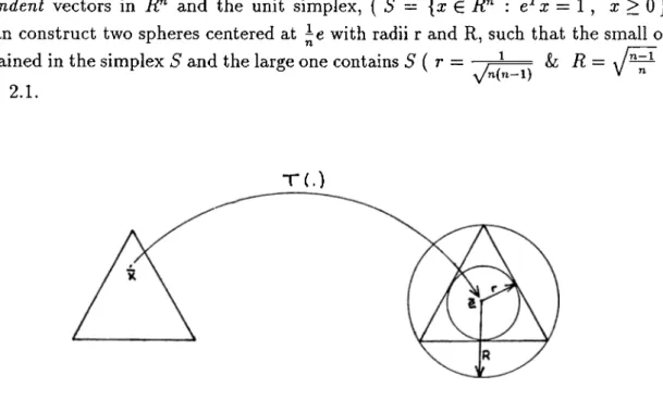
where L is the length of input data. In each iteration, the algorithm utilizes a projective transformation, r ( .) , from simplex S onto itself, such that the current interior point, x’, is mapped to ^e, the center of the simplex, S. Simplex is the polytope defined by n+1 affinely
independent vectors in i?" and the unit simplex, ( 5 = {x 6 jR" : e^x = 1 , a; > 0 } ) One can construct two spheres centered at with radii r and R, such that the small one is contained in the simplex S and the large one contains S i r — - , - — L· R = \ )
^ * '' V n (n -l) V n )
see fig. 2.1.
T ( . )
Figure 2.1: The projective transformation from the unit simplex S in i?" onto itself.
If the current point is the center of S', then feasibility is always preserved by moving at most r units along a feasible unit direction p, i.e. p satisfies Ap = 0 e^p = 0 || p ||= 1. Then the algorithm is given as follows:
0) Initialization, = 0 , x° = ^ e .
1) Optimality check. If c^x* < 2~^ STOP, otherwise continue. 2) Basic iteration.
i) B = AD
ii) Pn(b) = I - B ' ^ { B ' ^ B ) - ^ B
iii) p = Pn(b) Dc
iv) 2/ = i e + , where a < r.
v) x*'+^ = where T(x,x*') = jD is an n x n diagonal matrix with diagonal entries are; Du = xf.
Since our original cost function, c^x is not invariant under projective transformations, a somehow different cost function, named as “Potential Function”, /(c, x) = l o g ( ^ ) , which is invariant under such transformations is used. It is shown that, in every iteration at least a constant amount reduction, 6 which is independent from the problem data, in potential function is guaranteed. Using the stopping criterion which will be discussed in the next chapter, it is concluded that the number of iterations is O (nL). In each iter ation, 0 (n^) arithmetic operations is required to perform the matrix of projection onto the N{A). Those make the total time complexity of Karmarkar’s Algorithm o (tAL). In contrast to both, the Ellipsoid Algorithm and the Simplex Method, the round-off errors in each iteration is not accumulated in the Karmarkar algorithm, and this is a very good feature for the computer implementations.
After the presentation of Karmarkar, a large number of studies on the subject of the projective algorithm were published. Those studies can be classified in two groups : i) those taking the advantage of the sparseness of the large scale LP problems [1, 24], ii) those using approximate projection [3, 14, 21].
A well known variant of Karmarkar’s algorithm was reported by M.J. Todd L· B.P. Burrell [26], in 1985. They combined the duality theory with the interior point approach and used the dual variables to get an estimate for the optimum value, as a lower bound. This was a relaxation on the first assumption, and as a result of it, the variant could solve the problems with unknown objective values. Another practical improvement that they introduced was to generate the basic point solutions [not necessarily feasible) at any desirable iteration with a very modest extra cost.
A variant of the Karmarkar’s Algorithm for problems in standard LP form was intro duced by D.M. Gay [10], in 1987. The standard form LP is defined as;
S P ) min (Fx
s.t. A X = b X > 0
where A, b, c, and x have the same sizes as in P. The variant requires no apriori knowledge of the optimal objective function value. It uses a similar approach with Todd and Burrell [26] to compute the more strict lower bounds for the optimal value. Besides the elimination of the first assumption, the variant works exactly as the original algorithm. It utilizes the exact projection, and it stops when the “gap” between the current objective value and the lower bound is reduced to e = 2“^.
In 1988, D. Goldfarb L· S. Mehrotra [13] reported a relaxed variant of Karmarkar’s Al gorithm. They used the similar LP family L P (z) with Anstriecher [3], for the transferred problem formulations.
L P (z ) min (c — zdYX s.t. A X = 0
e^x = 1
X > 0
where d = the current iterate solution. The relaxed problem L P (z) is solved using approximate projection. The new iterate point is x^'^^ = T~^{y, d) where y = e +
0 < Q' < 1 and p € jR" is a decent direction. They called (p, z) as an admissible pair if the following conditions are satisfied; i) A'p = 0 , e^p = 0 and p ^ 0,
ii) { c — zd ) ( e + ) < 0, where A' = AD , c = Dc and Z) is a n x n diagonal matrix with D{i,i) = x,^ i = 1,2, ...,n . Using a Congugate Gradient (CG) technique p = Z' w{ c) , the decent vector, is generated approximately from the least square problem ||Z'te(c") — c’ll where c ” = {Dc — zd) , w{c) G BA and Z' is the basis matrix of N{A!). Basic linear algebra knowledge gives us a simple representation of the basis of
, where B and N are the partitions of the matrix A.. Therefore,
N{A) as Z =
Z' = - D b^B-^
I N Dn
where Db and Dn are the partitions of the diagonal matrix
D as D If the generated (p, z) pair is not admissible, then either a
/
Db 0
0 Dj^
more accurate projection vector p' is required, or a more strict lower bound z', where
z < z' < z* is needed. If a CG technique is used, the more accurate projection vector p ' can be easily obtained by continuing on iterations on least square problem from where
it was temporarily stopped, instead of recalculating it from scratch. Also, the updated lower bound z' = z A A , A > 0 can be calculated using the information of approximate CGLS solution.
Performance of the Karmarkar’s algorithm and its variants are highly dependent on the stopping criteria. One way of improving the stopping criteria is to identify the optimal basis as early as possible. Recent studies are mostly related with this early identification schemes. Gay [11], Kovacevic [22], Tapia [25] and Ye [28] use very similar techniques to form the optimal basis in their studies. The simplest one is due to Tapia and Zhang [2.5]. They define an indicator vector q, which is the diagonal entries of the matrix of projection to the row space of the constraint matrix, R(A). And it is stated that this indicator vector convergence to a 0 — 1 vector, which indicates whether the variable is nonbasic or basic at the optimum solution quadraticly faster than the convergence of the interior point solution to the optimum solution (i.e. — q*\\ < 0 (||.x^ — x’ lH ). These stopping rule implementations will be discussed in the Appendix B briefly. Also, in the late seventies M.C. Cheng presented an early optimum basis identification scheme for the Simplex Method [29].
In 1986, M. Kojima [20] reported that it is possible to determine the basis of the optimal solution before the algorithm satisfies the stopping criterion. This reduced the number of iterations in some problems, but he could not manage to put a limit to the number of iterations. In the same year, Kojima &: Tone published a modified version of the Karmarkar’s Algorithm [21]. Besides the optimum basic variable test, they presented a test for nonbasic variables at the optimum solution, as well. They used approximate projection in this variant and obtained some good results.
3.
K A R M A R K A R ’S A L G O R IT H M
The algorithm was announced at the Symposium on Theory of Computing by N. Kar- markar, in April 1984. In the worst case the algorithm requires o {n‘^L) arithmetic op erations, where n is the dimension of the problem and L is the input data length. The algorithm works on the special type of LP problems over rational data, call it K P (defined in Chap. II). After the projective transformation T{x,d) = gT£)-i^ iii the image space an equivalent problem K P is defined as;
K P ) min c^y-T
s.t. Ay = 0 e^y = 1
i/ > 0
where c = Dc , A = AD, and D is diagonal matrix with Da = d, and d € int(ICV), i.e. an interior point of the problem KP. The potential function which is invariant under projective transformation is defined
n
$(c, x) = n log c^x — ^ Iog(a;j) i=i
and in the image space $(c, y) = $(c, x)-\-\og[Det{D)], where y = T(x, d). This invariance will lead the number of iterations in the algorithm be polynomial, if at least a constant amount reduction in the potential function is guaranteed in the image space.
Theorem 1: For a G (0,1) , there exist a 8[a) > 0 such that.
$(c,?/) - $(c,e) < -8{a) , where e = -e and y = e — arn Pc
The proof of theorem 1 is given at the Appendix A in details. Using this main result, the following theorem concludes that the algorithm has a polynomial time complexity.
Theorem 2: Let n be the dimension of the problem K P and L be the input data length. Under the given assumptions in Chap. II, Karmarkar’s Algorithm will obtain an interior vector X satisfying
c^x < 2~^ ( 1)
in at most O (nL) iterations.
Proof: Let us start with the interior vector, a;° = e. After k iterations we get another interior point a;^, and a k8{a) reduction in potential function. So,
$ ( c ,x * ) - $ ( c ,e ) < -kS{a)
Using the definition of potential function
n log ^ log X* + n log n - kS{a) i=i
Or,
where Kq = nc^e = YJj-i cj and for k = o {nL) Equation 4 becomes, c^x^ < e~^ < 2~^
(2)
(3)
(4)
□ .
Moreover the stopping criterion guarantees us that any basic feasible x vector satisfies
c^x < c^x will be an optimal solution to the problem K P . It is a very well known fact
that calculation of the projection matrix P in each iteration is of O {n^). This concludes that the Karmarkar’s Algorithm is a polynomial algorithm, and its worst case bound is of the O {n*L). But in most variants this is reduced to O using approximation techniques in the step (2 ii). Depending on the implementation the algorithm could run even 50 times faster than the Simplex Method for large scale problem instances [1, 17, 24].
4. S IM P L E X T A B L E A U B A S E D A P P R O X IM A T E
P R O J E C T IO N A L G O R IT H M
In this chapter, a new variant of Karmarkar’s Algorithm, Simplex Tableau Based Ap proximate Projection (STBAP) Algorithm will be discussed. As its name implies, this variant uses approximation in calculating the projection matrix like many other variants of Karmarkar Algorithm. In STBAP Algorithm, the Simplex Tableau (ST) information is embedded into the approximation rule. Also, an early termination with an optimum ST is another advantageous feature of the algorithm.
Our algorithm works on the canonical form LP problems
L P min c^x
s.t. A x = h
X > 0
with the following assumptions:
i) LP has an optimum value of zero. ii) Constraint matrix, A is of full row rank.
iii) The center of the unit simplex in RP· is feasible.
In order to convert the problem L P into K P and be sure that it satisfies all the as sumptions, the A and c matrices change, and the new problem LP is:
L P min c^x
s.t. Ax = 0 X > 0
where = [c^, —z*], z* is the optimum objective value of L P , A = [A, —6] and x € with x\:n = X and x„+i = 1 (constant). Since x„+i has to be fixed to one, the inverse trans formation is defined as; T~^{y,d) = where d and D are defined in the previous
chapter. In L P , there is no constraint as e^x = 1, because after the transformation T(.), the equivalent problem K P in Y-space (image space of the transformation T(.)) always satisfies the constraint, e^y = = 1, and the optimum value of the problem LP
z* = 0). After the formation of the problem L P, the ST of the
is zero (c·“®* = c^x
(
problem is constructed by using a partition of constraint matrix, A = [jB, N] where B is a nonsingular square submatrix of A.
4.1
S im p lex T ableau
Since K P has a special structure, ST looks different than the ones in the Simplex Method. There is no need to carry the “rhs” vector and to calculate the objective value, since “rhs” is a vector of zeros and the basis is not necessarily feasible. Thus, the “rhs” column (i.e. the last column) of the original tableau can be eliminated. Therefore, the built ST occupies a place of (m + 1) X (n + 1) instead of (m + 1) x (n + 2) in the memory. Due to the construction of K P from L P , the first element of the last column of the ST gives the gap between the optimum value and current basic solution’s objective value, and the remaining elements in the last column represent the current basic solution in opposite sign.
S T )
cn — cbB —z* -|- cbB ^b B - ^ N - B - H
where cb and Cjv are the appropriate partition of the cost vector, c with respect to the
partition of A. R e su lts:
1. The current basis is feasible if and only if the last column of the ST is non-positive. 2. The current basis is optimal if and only if both:
i) the last column of the ST is non-positive, ii) the first row of the ST is non-negative.
which means, the last element of the first row is equal to zero. This makes sense, because if the basis is optimal then Xg = B~^b , cb^b ~ CBB~^b = z*.
In order to transform ST into the image space, Y-space, replace B by B Db , N by NDj\f, Cb by cbDb and cyv by cnD^. Since Xn+i = 1, there is no need to modify b. Then
STy looks somehow different but it gives exactly the same information, because both Db
and Dn are positive diagonal matrices.
S T y )
(cyv — cbB ^N)Dn Db^ B - ^ N Dn
- z · + CBB-'^b - D g ^ B - ^ b
Again the same results are valid for the STy. STy has the same space requirement and time complexity in build up as the original ST used in the Simplex Method; space(STy) is O (mn) and time(STy) is 0 {rn^n). STy has to be updated in each iteration due to the changes in matrices Db and and this updating is O (mn) simple multiplications.
Besides these regular updates, in some iterations the basis is changed to ensure the basis matrix, B Db be well-conditioned.
Since approximate projection is utilized, in some iterations the constructed direction is not admissible (i.e. it could not guarantee the minimum reduction 6 in potential function), and exact projection is required. In order to prevent the bad effects of the ill-conditioned basis matrix over the constructed decent direction, the basis representation of N(A) is changed (i.e. the basis of the ST), before the exact projection. This ST change means that a new basic feasible solution is reached. First, it is checked whether it is the optimum solution or not. If the optimum basic feasible solution is not reached, a new interior vector is found via line search over the potential function between the current solution and the new basic solution. This type of tableau update is O (n^m). For assuring the numerical stability the pivot rule used in finding the basic solution is different than the one in the Simplex Method.
T h e p iv o t ru le is:
Since the current solution is strictly positive, while entering a nonbasic variable into the basis it is possible to decrease it as well. Therefore, every nonbasic variable enters the basis ones, by increasing or decreasing its value. For the leaving variable, among the variables with non-zero entries in ST at the required column (i.e. the column of the entering variable) choose the one which has the smallest value in the current interior solution, so that the basis matrix will be kept well-conditioned.
4.2
P r o je c tio n o n to N{ A)
In each iteration of the Karmarkar’s algorithm, the transformed cost vector in Y-space have to be projected onto the null space of constraint matrices in Y-space to get an admissible moving direction, p — Pj^^^ad^Dc . If the exact projection is applied to the
vector D c the direction is:
P = I - D A ^ \ A D ^ A ^ ) - ^ A D - —ee
n Dc
Let M = DA'^(AD^A^)~^AD, then AIDc is the costly term of the calculation of the direction vector, p. It requires O (n^) arithmetic operations whereas the other terms require O (n).
Since in each iteration the D matrix changes, M has to be recalculated, and its time complexity directly effects the overall performance of the algorithm. Therefore several methods, like Least Square, Chelosky Factorization, etc... are used to calculate the M D c approximately, and reduce the time complexity of the algorithm.
The STBAP Algorithm also utilizes approximate projection, but contrary to most approximation techniques the scheme used causes only very small round-off errors, like the implementation of Goldfarb & Mehrotra [13]. Because the idea is not to approximate the space, A^(A), but to use a proper subsection of it, r)(A) C N{A).
Let p = ( I — M)Dc , then another representation of the direction vector is ;
p = ZZ^Dc^ where Z is n orthonormal basis of N{A). The simplex tableau basis of - D I ^ B - ^ N Dn
and it is orthonormalized by Gram-Schmidt tech-N(AD) is Z =
1
nique to form Z. One can calculate the exact projection over Dc using the whole nullspace basis, Z. In the case of approximate projection a subset of the basis vec tors is used. Basis vectors are the columns of Z i.e. z*. Then the approximate direc tion is; p = Zk ZjD c, where Zk = {z' : i £ Ik } , and 0 < < 1 is the approxima tion coefficient, and h C {1,2, ..,n — m}. In the implementation Ik is chosen such that ; I k = {i : i = i i , , \cji\ > \cj2\ > ... > |cj;| > ... > |cj(„_„,)| , I = [A:(n - m)J }, where
C{ denotes the reduced cost of variable i. Therefore, p = z'z''^Dc is the direction
calculated in a k-approximate projection iteration which has a time complexity of 0 {Pn).
4.3
S to p p in g C riteria
The STBAP algorithm terminates due to the “Simplex Tableau Test” (STT) or the orig inal stopping criteria which is also utilized in the standard Karmarkar Algorithm imple mentation as well.
The algorithm is stopped by STT if the current ST basis is the optimum basis. STT gives a positive answer if i) the first row of the ST is nonnegative, ii) the last column of the ST is nonpositive.
4.4
T h e A lg o rith m
In the previous section the termination of the algorithm is discussed. But in order to commence the iteration a strictly positive solution vector, x° is required. In the algorithm this difficulty is solved by using the “Big-M” method. First, the dimension of the problem,
n is increased by one. Secondly, the constraint matrix and cost vector are modified as; A = [A, b — Ae], c = [c, AI] where M e i? is very farge number. Then = e G is a strictly positive solution to the new problem, and it releases the assumption (iii). Since
AI is very large at the optimum solution, x*^j = 0.
After the conversion of the problem into LP, the algorithm starts with the initial interior point, x° = e and a partition of the constraint matrix, P A = [B, A^], where B is any nonsingular m x m submatrix of A and P is a permutation matrix, which will be ignored throughout the section. Using the partition initial ST is constructed and its optimality is checked by STT. Unless the optimum basis is attained the iterations are commenced. STy is built using the current interior solution, x*. Then, approximate projection scheme is applied to the Dc vector and a feasible direction, p in Y-space is calculated. The feasible direction is first tested if it is a decent direction by calculating the directional derivative of the potential function at the center of the simplex. If it is a decent direction, the step size, a along the direction via line search is found, and the reduction at the potential function due to the decent direction with the found step size is calculated. If the reduction is above a preset value, in the implementation it is taken
bmin = 0.1, the new iterate point in Y-space, y = e — arp a G (0 ,1) is back transformed to get the next interior solution, x*"*·^. Then the next iteration starts.
But, in the case where at least one of the two tests fail; i) the basis changes by means of the pivoting rule defined in the “Simplex Tableau” section and the new basis is checked for optimality by STT, ii) if the optimal basis is not achieved an exact projection scheme is done in the next iteration. Then the algorithm continues on iterations using approximate projection again.
The itemized structure of the STBAP Algorithm is given as follows:
0) Initialization. Choose a nonsingular basis of the constraint matrix, A. If it is the optimal basis, STOP
else, set A: = 0 , flag = 0 and start iterations.
1) Calculate the STy. If flag = 0 goto (2), else goto (3).
2) Approximate Projection. Using the reduced cost information, select a subset of feasible directions, and project the cost vector onto the subspace defined by the chosen directions, p = Papp Dc .
Goto (4).
3) Exact Projection. Using the ST calculate the orthogonal basis of the N(AD) and the projection matrix Pn(ad)· Project the cost vector onto N{AD), p = Pn(ad) Dc
4) Project p onto N ( e ^ ) , p = P;v(er)P and calculate the directional derivative due to
p at point ^e.
If the directional derivative is negative, goto (6).
5) Using ST find a basic solution (bfs) which has a better objective value than the current interior point, a:*'.
Apply STT; if it is the optimal basic feasible solution (bfs), STOP
else i) find a better interior point via line search between the current point and the found bfs; ii) set flag = 1 goto (1).
6) Calculate the step size, a and find the new interior point,
xkJrX _ ^ xky A: = + 1 and goto (1).
5. C O M P A R IS O N and R ESU LTS
In order to compare STBAP Algorithm with the standard version of Karmarkar’s Algo rithm, two computer programs were coded in C language. The implementation by D. Gay was chosen as the standard Karmarkar Algorithm. In both codes the same data struc tures were used (i.e. neither of them utilize the sparsity or structure of the problem and no preprocessing was done in both of them). Test problems are randomly generated in laboratory. The generated problems are in two different densities, 10% and 80%. First, A matrix is built via the given density by random numbers generated between —10 and 10. Then the rhs vector is calculated as 6 = Ae, so that problem is always feasible and satisfies the assumption (iii). The cost coefficients are calculated between the limits —99 and 99 with a density of 40%. In order to construct the L P problem, the value of the generated problems re calculated by using MINOS 5.0 on Data General MV 2000 mainframe. And for the computations the Sun Workstations were used.
The results of both algorithms are stated in the tables 1-2 and figures 1-4 at Appendix C. In the tables the following abbreviations are used. “App. Percent” : Percentage of approximation, lOOfc {k is the approximation coefficient). of ST change” : Number of basis changes during the algorithm. “7^^ of Exact Proj.” : Number of iterations that exact projection scheme is done. “Total iter.” : Total number of iterations. “Termination” : In termination the stopping criteria; CS means optimum ST cause the termination, G means the gap between the optimum and current objective value is less than e = 1 x 10~®, I L l & IL2 are used for termination due to iteration limit with a success or a fail to get the optimum, solution respectively. Where the iteration limit is taken as 51. The results due to the 100% approximation form the class of problems solved by the standard Karmarkar Algorithm.
If the completion times are compared (see the figures 1 L· 2), STBAP algorithm seemed to be advantageous for all the approximation schemes. This big difference is due to the time spend on calculation of the whole projection matrix in the standard implementation, whereas it is rarely calculated in the STBAP algorithm. In the last two figures, the total iterations and the number of iterations with exact projections (EP) are given. In terms
of the iterations, the low (10%) app. and the high (75%) app. schemes have closer total iterations to the standard implementation. As expected, the number of EP iterations de creased as the approximation coefficient k, increase. Because the approximated projected vector is closer to the exact projected vector as the approximation coefficient increases, of course the time per iteration increases as well. The best approximation scheme is seemed to use a low approximation coefficient (less than 20%, like 10%).
6. C O N C L U S IO N
In this study, it is tried to use the Simplex Tableau information in the implementation of Karmarkar Algorithm. Two computer programs are coded in order to compare this imple mentation with the standard implementation by D. Gay. The results of the comparison between the ST B A P Algorithm and the standard Karmarkar Algorithm implementation, shows that the idea of embedding the ST information into the interior point algorithms is promising. Therefore, a better computer code of the algorithm is needed to carry on the studies over the large scale problems. Also, the first assumption that the optimum value of the problem is zero has to be relaxed.
In the future, the possible research topics are:
• Investigate the best frequency of the basis changes in ST.
• Cooperate the stopping criteria discussed in App. B with the STRAP Algorithm and find the most compatible one with the algorithm. •
• Is it applicable to use a size reduction scheme in the STBAP Algorithm?
A . P R O O F OF P i;L Y N O M IA L IT Y OF T H E
K A R M A R K A R A L G O R IT H M
It is the bound on the number of iterations which makes the algorithm polynomial. In this section we will try to investigate why the algorithm stops in at most o{nL) iterations [2]. The stopping criterion is:
< 2 "^
For simplicity I will use c , e , P instead of c , , and projection onto the null space of B , Pn{b) matrices, through out this section.
Lemma 1: Let X = e + N{B) = { r 6 : Ax = 0 , e^x = 1}. Then G N{B) s.t.
G u ^ X , c^e ^ c^ti.
P roof:
Wx £ X X = e P Xo Xo ^ (1)
VXo G (? X = <F{PXo) = {(FP^)XoT dT \ = (Pc)^x (2)
Therefore,
X = c" e + {Pc)^x° 'ix £ X
(3)
Since the feasible region in the image space is contained by the ball B{e,R) in X , and
—Pc is the minimizing direction in Biß, R) projected onto X , for the function f ( x ) = c^x, Pc
/ ( e — Ru ) < f { x * ), where u =
Or, c^e — R(Pc)^u < c^x* = 0, by eqn. 3 . Since R = < 1 3.nd (Pc)'^u c^u > 0 ,
c^e — (p-u < c^e — Rc^u < 0
7^ — 7^
c e < c u
□ .
(4)
Lemma 2: For ||a;|| < /? < 1, we have the inequalities,
X —
2(1 -/? ) 2 < log (1 + x) < a: .
(5)
P ro o f: Let F[t) = log (1 + i) . By the Taylor’s theorem,
F(t) = F(0) + F '(0 )i + ^F"{0)F f o r some\e\ e (-/3,
Then
log(l + t) = t
-2(1 + 0)2
Since 1 + 0 > 1 — P and 2{i+e)'^ — from the equality
F t
-2(1 + 0)2 < log (1 + i) < t
□ .
Theorem 1: For a G (0,1), there exist a 0(a), depending only on a such that,
$(c,y) - $(c,e) < 0(a) (6)
Pc _ 1 .
P roof: Putting y = e — au , u = ---, e = - e into the LHS,
\\Pc\\
where a < r = ^ f o r n >> 1.
$(c, y) — #(c, e) = n log(c^e — 6t<Pu) — ^ log(e — au)j
i = i n 2 -n log c^e -j i n i = l = nlog < T - ^ T \ n e — ac^ u ' c^ e — ^ log(ne — nau)j i= i By lemma 1, nlog < T- A T > e — ac^ u P ' e < nlog(l — a)
(7)
(8)(9)
20^ log(ne - nau)j = log(l - ащ )
j=i j=i
Using lemma 2 and changing a by Equations 9 and 10 turn out to be;
fc^E — a c ^ u \
n log I --- 7WZ--- I < —Oi c^e
a^Uj - Y l o g ( n e - n a u ) j < Y ~o^uj + Л2
Since auj < and и G N (e^) is an unitary vector Equation 12 becomes,
^ < Y-OCUJ + a^Uj
4,2
< Q
2(1 — o:)^ Put Equations 11 and 14 into Equation 8,
Ф(с,?/) - Ф(с,ё) < -¿ (а ) where <5(a) = a - > 0. □ . (10) (11) (1 2) (13) (14) 21
B . S T O P P IN G C R IT E R IA
In this section, some of the stopping criteria rules by D.Gay [11], V.V.Kovacevic-Vujcic [22], Y.Ye [28] and Kojima [20] will be discussed. The rule by R.A. Tapia [25] was stated in chapter 4.
M. Kojima [20] stated a sufficient condition for a variable of a LP to be a basic variable at all optimum solution. He worked on the canonical LP for Karmarkar’s algorithm, K P . The proposed conditions are:
• rank = m + 1, for A
• a;* G int{}CV), where int(fCV) is used to indicate the set of interior points of problem KP.
• > 0.
• c^x* < 0.
where (x*) is a sequence of vectors in and x* is the optimum solution vector.
Indeed, these conditions are satisfied by the sequence of interior points (x*^), generated by any proper variant of the Karmarkar Algorithm. Then, the test is:
For i = 1,2, ..,n define the piecewise linear function g* : R ^ R
s.t.
g'{n) = m in |c^ + i ^
where P' denotes the column of the projection matrix, P and d’ = PDc.
Suppose that
g'{p) > 0 fo r some ^ > 0 , then X,· > 0 for any optimum solution.
The proof is given in the related paper by a contradiction. It is stated that the test is not effective for the first k iterations and the value of the k can be estimated by intuition.
V.V. Kovacevic-Vujcic [22] proposed a sequence of vectors (i*) related to the sequence (x^) generated by an interior point method have a higher degree of convergence to the optimum solution x* than the original interior point solution (x^). It is stated that different interior point methods share the same property that the normalized sequence of
lt+1 k
the search directions ^Txk+iZcTxk converges to the same direction.
Let us consider the Karmarkar’s canonical form problem, KP with his assumptions^ and a sequence of interior points, (x*). If (x*) satisfies the following conditions:
• x ’^ E int(fCV) A; = 1,2,... • x*·*·^ x^ A: = 1,2,...
• limfc_^oo 3;* = X, where x £ K P .
• limjt-fc->oo .*+1 -k = S
• 3 r > 0 s.t. X — ts > 0 , 0 < t < T
then the procedure of generating the auxiliary sequence (x*') is:
+ - I * ) ¿ = 0,1,...
where a* = m in ^ — xf < 0 i = 1,2, ..,n |.
D. Gay presented a method based on the “complementary slackness” idea for finding the optimum basis. Let P and D defines the primal aind dual problems respectively.
P = min{c^x : Ax = b , x > 0} D = {b'^y : A^y < c}
and the dual slacks are;
s = c — A^y > 0 .
Then the complementary slackness conditions imply for the primal and dual optimal solutions, X* and s*;
x*^s* = 0 .
The triple ( x, y, s ) is called “strict complementary triple” if x + s > 0, besides the third equation.
Using the above definitions, the stopping test for a primal-dual problem pair (P, D) which have a strict complementary triple is to search for a basis;
^In the original paper both the problem and the vector sequence are in general form
B = {1 < i < n : limyt_oo 7^ = °°} = ^ linifc—oo ^ = 0}. This test is very suitable for the primal-dual algorithms.
In the implementation a small enough threshold value, r > 0 has to be decided so that ^ B = {i : ^ "t} will give the optimum basis at iteration k. The crucial point is
the problem dependence of the the threshold value, r. This difficulty could be solved by rescaling the constraint matrix, A.
Y. Ye proposed a built-down scheme for both the Karmarkar Algorithm and the Sim plex Method. This is a size reduction procedure applied to the problem until the size reduced to rank(A) = m (in case of non degeneracy), i.e. the optimum basis is reached. The scheme commences with the “optimum basis candidate” set, which is all the columns of the constraint matrix, A at the beginning. Then the columns are monotonically elim inated via a special pricing rule. The pricing rule is based on the ellipsoid theory. The dual ellipsoid that contains all the optimal dual slacks is searched, and using the comple mentary slackness conditions:
s*x* = 0 Vi < n, one can identify the nonbasic variables at any optimal solution.
For the primal-dual pair (P — £>), with the assumptions of Karmarkar, let’s define the transformed primal problem, P;
P = r a i n { ^ x : Ax = 0 x > 0}
where A = [A, —6] and = [c^, —z*] with z* is the optimum value of the problem P. Thus, the optimum dual slacks set is defined as;
P * = {s* G : s* = c - A ^ y , y e R ^ }
M.J. Todd [27] derived that the ellipsoid that contains all the optimum dual slacks is;
||Ps*|p < (e^Ps*)2 = ( c V - z * ) 2
where D is the diagonal matrix defined by
diag(x^) 0 D =
0 1
We know that in any optimum dual solution the slack variable 5* > 0 implies that x* is nonbasic in any primal solution. Therefore, the minimum value of every slack variable has to be calculated. Indeed, one has to solve the following optimization problems for
i = 1,2, ..,n. E O P ) min. Si s.t. s = c — A^y
||Z)3|| <
where = (c^x* — z*). 24If the minimum value of the problem E O P is positive for some i, then the corresponding variable in primal problem, a;,· is nonbasic in any optimum solution. Thus the column of the constraint matrix can be eliminated from the “candidate” set.
C. R E SU L T S OF T H E T E ST P R O B L E M S
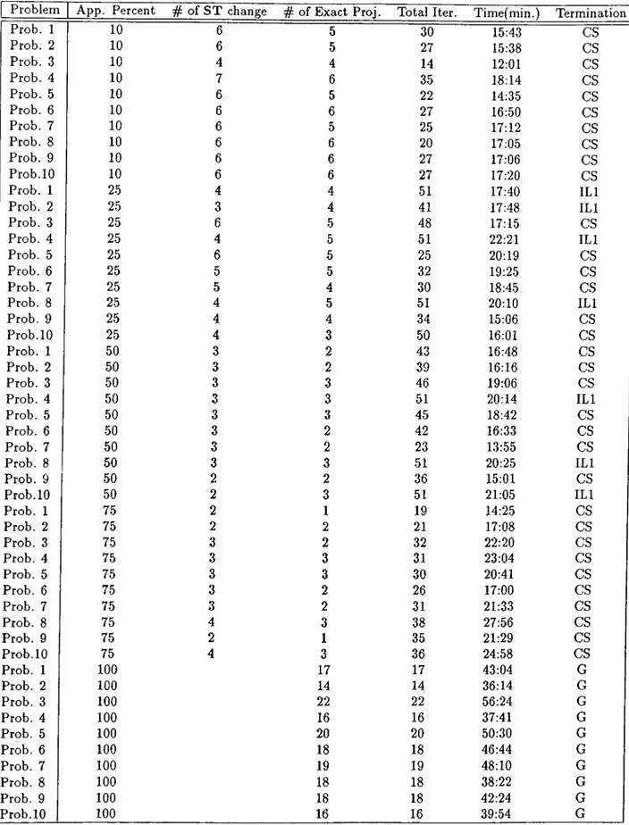
In this section the results of the both algorithms and the graphs demonstrating the per formance of different approximation schemes are given. In the tables the following ab breviations are used. “App. Percent” ; Percentage of approximation, 100^ (k is the approximation coefficient). of ST change” : Number of basis changes during the algorithm. of Exact Proj.” : Number of iterations that exact projection scheme is done. “Total iter.” ; Total number of iterations. “Termination” : In termination the stopping criteria; CS means optimum ST cause the termination, G means the gap be tween the optimum and current objective value is less than e = 1 x 10“®, I L l L· IL2 are used for termination due to iteration limit with a success or a fail to get the optimum, so lution respectively. Where the iteration limit is taken as 51. The results due to the 100% approximation form the class of problems solved by the standard Karmarkar Algorithm.
Problem App. Percent # of S T change Exact Proj. Total Iter. Time(min.) Termina 5 30 15:43 cs 5 27 15:38 cs 4 14 12:01 cs 6 35 18:14 cs 5 22 14:35 cs 6 27 16:50 cs 5 25 17:12 cs 6 20 17:05 cs 6 27 17:06 cs 6 27 17:20 cs 4 51 17:40 ILl 4 41 17:48 ILl 5 48 17:15 cs 5 51 22:21 ILl 5 25 20:19 CS 5 32 19:25 cs 4 30 18:45 cs 5 51 20:10 ILl 4 34 15:06 CS 3 50 16:01 CS 2 43 16:48 cs 2 39 16:16 cs 3 46 19:06 cs 3 51 20:14 ILl 3 45 18:42 CS 2 42 16:33 cs 2 23 13:55 cs 3 51 20:25 ILl 2 36 15:01 CS 3 51 21:05 ILl 1 19 14:25 CS 2 21 17:08 CS 2 32 22:20 CS 3 31 23:04 cs 3 30 20:41 cs 2 26 17:00 cs 2 31 21:33 cs 3 38 27:56 cs 1 35 21:29 cs 3 36 24:58 cs 17 17 43:04 G 14 14 36:14 G 22 22 56:24 G 16 16 37:41 G 20 20 50:30 G 18 18 46:44 G 19 19 48:10 G 18 18 38:22 G 18 18 42:24 G 16 16 39:54 G Prob. 1 10 Prob. 2 10 Prob. 3 10 Prob. 4 10 Prob. 5 10 Prob. 6 10 Prob. 7 10 Prob. 8 10 Prob. 9 10 Prob.10 10 Prob. 1 25 Prob. 2 25 Prob. 3 25 Prob. 4 25 Prob. 5 25 Prob. 6 25 Prob. 7 25 Prob. 8 25 Prob. 9 25 Prob. 10 25 Prob. 1 50 Prob. 2 50 Prob. 3 50 Prob. 4 50 Prob. 5 50 Prob. 6 50 Prob. 7 50 Prob. 8 50 Prob. 9 50 Prob.10 50 Prob. 1 75 Prob. 2 75 Prob. 3 75 Prob. 4 75 Prob. 5 75 Prob. 6 75 Prob. 7 75 Prob. 8 75 Prob. 9 75 Prob.10 75 Prob. 1 100 Prob. 2 100 Prob. 3 100 Prob. 4 100 Prob. 5 100 Prob. 6 100 Prob. 7 100 Prob. 8 100 Prob. 9 100 Prob.lO 100 6 6 4 7 6 6 6 6 6 6 4 3 6 4 6 5 5 4 4 4 3 3 3 3 3 3 3 3 2 2 2 2 3 3 3 3 3 4 2 4
Table C.2: Results of the problems of small size (50 x 100) with density 80%.
T 0 t. .1 1 ]' i ΙΤΙ t: íigqre C.l: figjæ С.2: 29
l n Figüre C-3: E P I t rî Figüre C.4: 30
R E F E R E N C E S
[1] Adler I., Karmarkar N., Resende M.G.C. and Veiga G., Data Structures and Program ming Techniques For the Implementation of Karmarkar’s Algorithm, Mathematical Programming 44, 297-335, 1989.
[2] Akgiil M., A Short Proof of Karmarkar’s Main Result, Doğa - Turkish Journal of Mathematics 14, 48-55, 1990.
[3] Anstriecher K.M., A Monotonic Projective Algorithm For Fractional Linear Pro gramming, Algoritmica 1, 483-498, 1986.
[4] Bland R.G., New Finite Pivoting Rules For the Simplex Method, Mathematics of Operation Research 2, 103-107, May 1977.
[5] Bland R.G., Goldfarb D., and Todd M.J., The Ellipsoid Method: A Survey, Opera tions Research 2, 1039-1091, 1981.
[6] Borgwardt K.H., The Simplex Method - A Probabilistic Analysis, Springer-Verlag, 1987.
[7] Dantzig G.B., Maximization of a Linear Function of Variables Subject to Linear Inequalities, Chap. XXI of Activity Analysis of Production and Allocation Codes Commission Monograph 13, T.C. Koopmer, John Wiley, New york, 1951.
[8] Edmonds J., Exponential Growth of the Simplex Method for Shortest Path Problems, University of Waterloo, 1970.
[9] Ford L.R.Jr. and Fulkerson D.R., Constructing Maximal Dynamic Flows From Static Flows, Operations Research Vol.6, 419-433, 1958.
[10] Gay D.M., A Variant of Karmarkar’s LP Algorithm For Problems in Standart Form, Mathematical Programming 37, 81-90, 1987.
[11] Gay D.M., Stopping Tests That Compute Optimal Solutions For Interior Point LP Algorithms, Numerical Analysis Manuscript 89-11, A T L· T Bell Laboratory, Dec. 1989.
[12] Goldfarb D. and Reid J.K., A Practical Steepest-Edge Simplex Algorithm, Mathe matical Programming 12, 361-371, 1977.
[13] Goldfarb D. and Mehrotra S., Relaxed Variants of Karmarkar’s Algorithm for Linear Programs With Unknown Optimal Objective Value, Mathematical Programming 40, 183-195, 1988.
[14] Goldfarb D. and Mehrotra S., A Relaxed Revision of Karmarkar’s Method, Mathe matical Programming 40, 289-315, 1988.
[15] Jeroslow R., The Simplex Algorithm With The Pivot Rule of Maximizing Criterion Improvement, Discrete Mathematics 4, 367-377, 1973.
[16] Karmarkar N., A New Polynomial Time Algorithm For LP, Combinatorica Vol.4, 375-395, 1984.
[17] Karmarkar N.K. and Ramakrishnan K.G., Implementation and Computational Re sults of the Karmarkar Algorithm for Linear Programming, Using an Iterative Method for Computing Projections, AT L· T Bell Laboratories, Research Report, 1988.
[18] Khachian L.G., A Polynomial Algorithm in LP, Soviet Mathematics Doklady 20, 191-194, 1979.
[19] Klee V. and Minty G.J., How Good is the Simplex Algorithm?, Mathematical Note no.643, Mathematics Research Laboratory, Boeing Scientific Research Laabs, Feb. 1970.
[20] Kojima M., Determinig Basic and Nonbasic Variables of Optimal Solutions in Kar markar’s New LP Algorithm, Algorithmica Vol.l, 499-515, 1986.
[21] Kojima M. and Tone K., An EfBcient Implementation of Karmarkar’s New LP Al gorithm, Technical Report No. B-180, Department of Information Sciences, Tokyo Institute of Technology, Japan, April 1986.
[22] Kovacevic V.V. and Vujcic , Improving the Rate of Convergence of the Interior Point Methods For LP, Faculty of Organizational Sciences, Belgrade University, 1989. [23] Lemke C.E., The Dual Method of Solving The Linear Programming Problem, Naval
Research Logistics Quarterly 1, 36-47, 1954.
[24] Oohori T. and Ohuchi A., An Efficient Implementation of Karmarkar’s Algorithm For Large Scale Linear Programs, Tech. Report, Hokkaido Istitute of Technology, Japan, Sept. 1988.
[25] Tapia R.A. and Zhang Y., A Fa^t Optimal Basis Identification Technique For Interior Point LP Methods, Technical Report No. 89-1, Department of Mathematical Sciences, Rice University, Oct. 1989.
[26] Todd M.J. and Burrell B.P., An Extension of Karmarkar’s Algorithm For Linear Programming Using Dual Variables, ALgoritmica 1, 409-424, 1986.
[27] Todd M.J., Improved Bounds & Containing Ellipsoids in K arm arkar’s Linear Pro gramming Algorithm, Mathematics of Operations Research 13, 409-424, 1988. [28] Ye Y., A Built-down scheme for Linear Programming, Mathematical Programming
Vol. 46, 61-73, 1990.
[29] Cheng M.C., New Criteria For The Simplex Algorithm, Mathematical Programming Vol. 19, 230-236, 1980.