On compact solution vectors in Kronecker-based Markovian analysis

(1)

Contents lists available atScienceDirect

Performance Evaluation

journal homepage:www.elsevier.com/locate/peva

On compact solution vectors in Kronecker-based Markovian

analysis

P. Buchholz

a

,

T. Dayar

b,

*

,

J. Kriege

a

,

M.C. Orhan

b a_{Informatik IV, Technical University of Dortmund, D-44221 Dortmund, Germany}

b_{Department of Computer Engineering, Bilkent University, TR-06800 Bilkent, Ankara, Turkey}

a r t i c l e i n f o

Article history:

Available online 24 August 2017 Keywords:

Markov chain Kronecker product

Hierarchical Tucker decomposition Reachable state space

Compact vector

a b s t r a c t

State based analysis of stochastic models for performance and dependability often requires the computation of the stationary distribution of a multidimensional continuous-time Markov chain (CTMC). The infinitesimal generator underlying a multidimensional CTMC with a large reachable state space can be represented compactly in the form of a block matrix in which each nonzero block is expressed as a sum of Kronecker products of smaller matrices. However, solution vectors used in the analysis of such Kronecker-based Markovian representations require memory proportional to the size of the reachable state space. This implies that memory allocated to solution vectors becomes a bottleneck as the size of the reachable state space increases. Here, it is shown that the hierarchical Tucker decomposition (HTD) can be used with adaptive truncation strategies to store the solution vectors during Kronecker-based Markovian analysis compactly and still carry out the basic operations including vector–matrix multiplication in Kronecker form within Power, Jacobi, and Generalized Minimal Residual methods. Numerical experiments on multidimensional problems of varying sizes indicate that larger memory savings are obtained with the HTD approach as the number of dimensions increases.

1. Introduction

Modelling and analysis of multidimensional continuous-time Markov chains (CTMCs) is an area with ongoing research interest. Handling of large state spaces is a major challenge in CTMC analysis approaches. When a system is composed of interacting subsystems, it may be possible to provide a state-based mathematical model for its behaviour as a multidi-mensional CTMC with each dimension of the CTMC representing a different subsystem and a number of transitions that trigger state changes at certain rates. The product state space size of such a model grows exponentially in the number of subsystems. In this kind of model, subsystems change state independently of states of other subsystems through local transitions, or they change state synchronously with one or more of the other subsystems through synchronized transitions. A subset of the Cartesian product of the subsystem state spaces forms the so-called reachable state space of the model. The reachable state space of such a model is determined by the combination of states in which the subsystems can be under local or synchronized transitions [1,2]. Usually not all states of the Cartesian product are reachable because transitions prohibit some specific combinations of subsystem states. However, in most models also the reachable state space grows quickly with an increasing number of subsystems. It is important to be able to represent this reachable state space and the transitions

*

Corresponding author.

E-mail addresses:peter.buchholz@cs.tu-dortmund.de(P. Buchholz),tugrul@cs.bilkent.edu.tr(T. Dayar),jan.kriege@cs.tu-dortmund.de(J. Kriege),

morhan@cs.bilkent.edu.tr(M.C. Orhan).

http://dx.doi.org/10.1016/j.peva.2017.08.002

(2)

among its states compactly and then analyse the stationary or transient behaviour of the underlying system as accurately and as efficiently as possible.

When the reachable state space at hand is large, the infinitesimal generator underlying the CTMC can be represented as a block matrix in which each nonzero block is expressed as a sum of Kronecker products of smaller rectangular matrices [3]. This is the form of the Kronecker representation in Hierarchical Markovian Models [1], where the smaller matrices can be rectangular due to the product state space of the modelled system being larger than its reachable state space [4]. When the product state space is equal to the reachable state space, the smaller matrices become square as in Stochastic Automata Networks [5,6].

For Kronecker-based Markovian representations, iterative analysis methods employ vector-Kronecker product multipli-cation as the basic operation [7]. The challenge is to perform this operation in as little memory and as fast as possible. When the factors in the Kronecker product terms are dense, the operation can be performed efficiently by the shuffle algorithm [8]. When the factors are sparse, it may be more efficient to obtain nonzeros of the generator in Kronecker form on the fly and multiply them with corresponding elements of the vector [2]. However, memory allocated for the vectors in these algorithms is still proportional to the size of the reachable state space, and this size increases exponentially with the number of dimensions.

The bottleneck of today’s numerical analysis methods for large CTMCs is the size of the vectors that need to be used. A more compact representation that avoids the complete enumeration of all reachable states would increase the size of solvable models significantly. An approach along this direction is the hierarchical Tucker decomposition (HTD) [9,10]. HTD was originally conceived in the context of providing a compact approximate representation for dense multidimensional data [11] in a manner similar to the tensor-train decomposition [12], but is more suitable to our requirements in that the decomposition is available through a tree data structure with logarithmic depth in the number of dimensions. Both decompositions have the special feature of possessing approximation errors that can be user controlled, and hence, approximations accurate to machine precision are computable using them. Clearly, with such decompositions it is always possible to trade quality of approximation for compactness of representation, and how compact the solution vector in HTD format remains throughout the solution process is an interesting question to investigate.

The tensor train decomposition has been applied in [13] to approximate the solution vector for models where the product space is reachable using an alternating least squares approach or the Power method. To the best of our knowledge, HTD was first applied to hierarchically structured CTMCs in [14]. Therein, it is shown that a compact solution vector in HTD format can be multiplied with a sum of Kronecker products to yield another compact solution vector in HTD format. Moreover, the multiplication of the compact solution vector in HTD format with a Kronecker product term does not increase the memory requirements of the compact vector, but the addition of two compact vectors does. This necessitates some kind of truncation, hence, approximation, to be introduced to the addition operation. To investigate the merit of the approach, the following analysis was performed in [14]. Starting from an initial solution, the compact vector in HTD format was iteratively multiplied with the uniformized generator matrix of a given CTMC in Kronecker form 1000 times. The same numerical experiment was performed with a solution vector the same size as the reachable state space size using an improved version of the shuffle algorithm [15]. For a fixed truncation error tolerance strategy in the HTD format, the two approaches were compared for memory, time, and accuracy, leading to the preliminary conclusion that compact vectors in HTD format become more memory efficient as the number of dimensions increases. We remark that compact representations for solution vectors in Markovian analysis have also been considered from the perspective of binary decision diagrams [16,17]. The proposed compact data structures therein have not been timewise competitive and do not allow the computation of truncation error bounds, whereas the approach investigated in [14] seems to be a step forward.

Here, we build on to the work in [14] by using the HTD format for solution vectors within the iterative methods of Power, Jacobi, and Generalized Minimal RESidual (GMRES) [7]. We are interested in observing how the memory requirements of the compact solution vectors in HTD format change over the course of iterations due to the sequence of multiply, add, and truncate operations in each iteration, together with the average time it takes to perform each iteration and the influence of the truncation error on the quality of the solution. Two adaptive truncation strategies for the HTD format are implemented and the performance of the resulting solvers compared on a large number of multidimensional problems with their Kronecker structured counterparts that employ solution vectors the same size as the reachable state space size. Results are encouraging, confirming the preliminary results in [14] and indicating that it is worthwhile to invest compact representations for solution vectors in higher dimensional systems.

Although we use in our research the basic algorithms from [9,10], we apply them in a different context. While [9,10] use simple and very regular examples, we apply the approach to Hierarchical Markovian Models with an irregular structure that are much more difficult to analyse. This implies that new strategies to perform truncation during the solution process need to be integrated into the iterative methods and new problems like the compact representation of the inverse of the diagonal of a matrix in Kronecker form need to be solved. Moreover, the original approach has been implemented as a MATLAB toolbox which is not geared towards the analysis of large hierarchically structured CTMCs. Therefore, we use a new implementation in C [18] as an extension of the NSolve package of the Abstract Petri Net Notation (APNN) toolbox [19,20].

The organization of the paper is as follows. In Section2, we provide background information on HTD and the related algorithms that are used in our setting. In Section3, we discuss the implementation framework and the iterative solvers used with the adaptive truncation strategies for the HTD format. In Section4, we present the results of numerical experiments with the NSolve package on a large number of multidimensional problems of varying sizes. Section5concludes the paper.

(3)

2. Compact vectors in Kronecker setting

Let

{

S(t)

=

(S1(t)

, . . . ,

Sd(t))

∈

R

,

t

≥

0

}

be the d-dimensional stochastic process associated with the evolution of a

system composed of d subsystems. Here,Shis the set of states that the hth subsystem (h

=

1

, . . . ,

d) can be in andRis

the reachable state space of the system satisfyingR

⊆

S, whereS

= ×

d_h₌₁Shis the product state space of the system. The

stochastic process

{

S(t)

,

t

≥

0

}

is said to be continuous-time Markovian if the memoryless property holds, which means that time to exit a state s

∈

Ris exponentially distributed with a rate that depends only on s and the transition probability to another state s′

_∈

Rdepends only on the source state s. WhenShcan be mapped to a subset of the set of integers for

h

=

1

, . . . ,

d, the reachable state spaceRbecomes denumerable and

{

S(t)

,

t

≥

0

}

is called a CTMC. The rate of a transition from state s

∈

Rto s′

_∈

Rcan be captured as the (s

,

s′

)th entry of an (

|

R

| × |

R

|

) matrix for s

̸=

s′

and s

,

s′

_∈

R. This matrix is called the infinitesimal generator of the CTMC and has off-diagonal entries that are nonnegative. The diagonal entries of the infinitesimal generator are equal to its negated off-diagonal row sums so as to represent the negated rates at which the CTMC remains in each state [7]. In the following we assume thatShis finite and defined on consecutive nonnegative integers

starting from 0 for h

=

1

, . . . ,

d.

WhenR

⊂

S, it becomes important to find a compact representation forRthat omits the states inS

−

R. Now, let

R(i)

= ×

d_h₌₁R(i)_h

,

whereR(i)_h is a partition ofS_hin the form of consecutive integers for i

=

1

, . . . ,

J. ThenR(1)

, . . . ,

R(J)is a Cartesian product partitioning [4] ofRif

R

=

J

⋃

i=1

R(i) and R(i)

∩

R(j)

= ∅

for i

̸=

j

,

i

,

j

=

1

, . . . ,

J

.

The (

|

R

|×|

R

|

) infinitesimal generator Q underlying the CTMC can be viewed as a (J

×

J) block matrix induced by the Cartesian

product partitioning ofS[3,4] as in Q

=

⎡

⎢

⎣

Q(1,1)

. . .

Q(1,J)

... ... ...

Q(J,1)

. . .

Q(J,J)

⎤

⎥

⎦ .

Block (i

,

j) of Q for i

,

j

=

1

, . . . ,

J is given by

Q(i,j)

=

⎧

⎪

⎨

⎪

⎩

∑

k∈K(i,j) Q(i_k,j)

+

Q(i)_D if i

=

j

,

∑

k∈K(i,j) Q(i_k,j) otherwise

,

where Q(i,_kj)

=

α

_k d

⨂

h=1 Q(i,_k_,_hj)

,

Q(i)_D

= −

J

∑

j=1

∑

k∈K(i,j)

α

k d

⨂

h=1 diag(Q(i,_k_,_hj)e)

,

⊗

is the Kronecker product operator,

α

kis the rate associated with continuous-time transition k,K(i,j)is the set of transitions

in block (i

,

j), e represents a column vector of ones, diag(a) denotes the diagonal matrix with the elements of vector a along

its diagonal, and Q(i_k_,,_hj)is the submatrix of the transition matrix Qk,hwhose row and column state spaces areR(i)h andR (j) h,

respectively [1].

There are a finite number of transitions that can take place in the system, and the set

⋃

J

i,j=1K(i,j)represents all possible

transitions. It is usually the case that some transitions are possible in some states, while others are possible in other states. Here,K(i,j)represents transitions that are possible when the system is in states ofR(i)and that take the system to states inR(j). IfK(i,j)

_{= ∅}

_{, then block Q}(i,j)

₌

_{0 for i}

_̸=

_{j. In practice, the matrices Q}

k,hare sparse [3] and held in sparse row format since the

nonzeros in each of its rows indicate the possible transitions from the state with that row index. The advantage of partitioning the reachable state space is the elimination of unreachable states from the set of rows and columns of the generator to avoid unnecessary computational effort (see, for instance, [2,15]) due to unreachable states and to use vectors not larger than

|

R

|

in the analysis. The Kronecker form of the blocks Q(i,j)_{in Q has been studied before for a number of models [}₂₁_–₂₃_{]. Since}

this work is not about the compact representation of generator matrices using sums of Kronecker products, we refer to these papers for more information. We also remark that the continuous-time transition rate of a Kronecker product term,

α

k, can

be eliminated by scaling one (perhaps, the first) factor in the term with that rate.

Matrix Q(i)_D is a diagonal matrix which is represented as a sum of Kronecker products of diagonal matrices. In iterative solution methods exploiting the Kronecker structure, diagonal elements are often stored in a vector as large as

|

R

|

which is multiplied elementwise with the iteration vector. This is timewise more efficient than multiplying a Kronecker product of matrices with the iteration vector. However, if the reachable state space is sufficiently large, the storage of vectors with size

|

R

|

is not feasible and the diagonal can instead be represented as sums of Kronecker products. This approach works

(4)

well as long as we use numerical methods that are based on multiplication of the iteration vector with the entire generator matrix. In methods like Jacobi, where the iteration vector has to be multiplied with the reciprocal of the diagonal elements, the Kronecker representation of an element cannot be easily transformed to a compact representation of the reciprocal of the element. This problem will be considered in Section2.6.

The core operation of most numerical methods for computing the stationary or transient distribution of CTMCs with large state spaces is the computation of vector–matrix products [7]. Thus, a time and, for large state spaces also, a memory efficient realization of this operation is the key step in performing quantitative analysis of large multidimensional systems. To simplify the discussion and the notation, we consider the multiplication of a single block of Q from the left with a (sub)vector, and therefore, omit the indices (i

,

j) and write the index k associated with the transition as a superscript in parentheses above

the matrices forming the block. Hence, we concentrate on the operation

yT

:=

xT K

∑

k=1 d

⨂

h=1 Q(k)_h

,

where Q(k)_h is an (mh

×

nh) matrix, implying

⨂

d h=1Q (k) h is a (

∏

d h=1mh

×

∏

d h=1nh) matrix, and x is a (

∏

d h=1mh

×

1) vector. K

is equal to the number of terms in the sum, i.e.,

|

K(i,j)

|

if we consider block (i

,

j). Observe that this is the operation that takes

place when each block of a block matrix in Kronecker form such as Q gets multiplied on the left by an iteration subvector. In fact, the same subvector multiplies all blocks in a row of the matrix in Kronecker form.

To be consistent with the literature, we consider in the following multiplications of Kronecker products

⊗

d h=1A

(k) h with

column vector x and their summation in the usual matrix–vector form

y

:=

K

∑

k=1

(

_d

⨂

h=1 A(k)_h

)

x

,

where A(k)_h is the transpose of Q(k)_h and of size (nh

×

mh). In particular, we are interested in its implementation as

y(1)

_:=

₀

_,

_x(k)

_:=

(

_d

⨂

h=1 A(k)_h

)

x

,

y(k+1)

_:=

_y(k)

₊

_x(k) _{for k}

₌

₁

_{, . . . ,}

_K

_,

and y

:=

y(K+1)_{, where 0 is a column vector of 0’s. Now, we turn to the HTD format.} 2.1. HTD format

The compact representation of the generator matrix using a hierarchical Kronecker form [1,3,5,6] was a first step in reducing the memory requirements of iterative numerical solvers. With this step, storage of the generator matrix becomes negligible for larger models. To further enlarge the size of numerically analysable state spaces, the memory requirements of iteration vectors need to be reduced as well. This is a difficult problem since there is no a priori known closed-form expression for the elements of an iteration vector of a large CTMC in Kronecker form. A natural choice is the use of the multidimensional structure also for the vector representation. However, since the compact representation of an iteration vector, in contrast to the compact representation of the generator matrix, usually will not be exact, it is important that one uses a representation that allows control over the resulting truncation error. In this way, it is possible to regulate the accuracy of the solution and indirectly the memory requirement by seeking less accurate approximations when far away from the solution and improving the accuracy of the approximations as the residual norm becomes smaller. Such a representation is the HTD [11] which will be presented next in the context of compact iteration vectors for multidimensional CTMCs.

Assuming without loss of generality that d is a power of 2, a (

∏

d

h=1mh

×

1) vector x in (orthogonalized) HTD format can

be expressed as

x

=

(U1

⊗ · · · ⊗

Ud)c

,

where Uhfor h

=

1

, . . . ,

d are (mh

×

rh) orthogonal basis matrices for the different dimensions in the model and c

=

(B_1,2

⊗ · · · ⊗

B_d−1,d)

· · ·

(B1,...,d/2

⊗

Bd/2+1,...,d)B1,...,d

is a (

∏

d

h=1rh

×

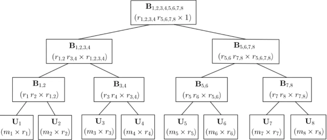
1) vector in the form of a product of log2d matrices each of which except the last is a Kronecker product of

a number of transfer matrices Bt. See the full binary tree ofFig. 1. The transfer matrix Btis of size (rtlrtr

×

rt) with the node

index t defined as t

:=

tl

,

tr, and r1,...,d

=

1 since B1,...,dis at the root of the tree [9,pp. 5–6].

The (d

−

1) intermediate nodes of the binary tree inFig. 1store the transfer matrices Btand its leaves store the basis

matrices Uhso that each intermediate node has two children. In an orthogonalized HTD format of x, one can also conceive of

orthogonal basis matrices Ut

=

(Utl

⊗

Utr)Bt, at intermediate nodes with rtcolumns that relate the orthogonal basis matrices U_t_land Utrfor the two children of transfer matrix Btwith the transfer matrix itself. In fact, the orthogonal matrix Uthas in its

columns the singular vectors associated with the largest rtsingular values [24,pp. 76–79] of the matrix obtained by taking

index t as row index, the remaining indices in order as column index of the d-dimensional data at hand (i.e., with a slight abuse of notation, x(

{

t

}

, {

1

, . . . ,

d

} − {

t

}

)). Hence, we have the concepts of ‘‘hierarchy of matricizations’’ and ‘‘higher-order

(5)

Fig. 1. Matrices forming x in HTD format for d=8.

Fig. 2. Matrices forming x in HTD format for d=5.

singular value decomposition (HOSVD)’’, and rtis the rank of the truncated HOSVD. Observe that the simplest case with all

ranks equal to 1 corresponds to a Kronecker product of vectors of length mhfor h

=

1

, . . . ,

d. More detailed information

regarding this can be found in [9,11]. We remark that Btmay also be viewed as a 3-dimensional array of size (rtl

×

rtr

×

rt)

having as many indices in each of its three dimensions as the number of columns in the matrices in its two children and itself, respectively. The number of transfer matrices in the lth factor forming c is the Kronecker product of 2log2d−l_transfer

matrices for l

=

1

, . . . ,

log₂d

−

1. In fact, c is a product of Kronecker products, and so is x, but neither has to be formed explicitly.

When d is not a power of 2, it is still useful to keep the tree in a balanced form and use the ceiling operator on the height of the tree, for instance, as inFig. 2for which

x

=

(((U1

⊗

U2)B1,2)

⊗

U3

⊗

U4

⊗

U5)(B1,2,3

⊗

B4,5)B1,2,3,4,5

.

Assuming that rmax

=

maxt(rt) and mmax

=

max(m1

, . . .,

md), memory requirement for matrices in the binary tree

associated with HTD format is bounded by dmmaxrmaxat the leaves, rmax2 at the root, and (d

−

2)rmax3 at other intermediate

nodes, thus, totally dmmaxrmax

+

(d

−

2)rmax3

+

rmax2 . In the next subsection, we show how a particular rank-1 vector can be

represented in HTD format.

In the next subsections, we discuss the ingredients that are related to the implementation of the multiplication of a sum of Kronecker products with a vector in HTD format so that it can be used in iterative methods. Therefore, other than the multiplication of a Kronecker product with a vector in HTD format and the addition of two vectors in HTD format, we need to show how the initial solution vector (which is normally taken as the uniform distribution) can be stored in HTD format and how the norm of a vector in HTD format can be computed so that it is used in the test for convergence. Finally, we discuss how the reciprocation of diagonal elements of the generator matrix in Kronecker form can be performed in HTD format so that it can be used in the Jacobi method.

(6)

2.2. Uniform distribution in HTD format

Let x

=

e

/

m be the (m

×

1) uniform distribution vector, where m

=

∏

d

h=1mh. Then x may be represented in HTD format

with all matrices having rank-1 for which the basis matrices given by Uh

=

e

/

√

mhare of size (mh

×

1) for h

=

1

, . . . ,

d and

the transfer matrices given by

Bt

=

⎧

⎪

⎨

⎪

⎩

(

_d

∏

h=1

√

mh

)

/

m if t corresponds to root 1 otherwise

are (1

×

1). Note that memory taken up by the full representation of x is m nonzeros, whereas that with HTD format is

d

−

1

+

∑

d

h=1mhnonzeros since the (d

−

1) transfer matrices are all scalars equal to 1 except the one corresponding to the

root. In passing to the multiplication of a compact vector with a Kronecker product, we remark that each basis matrix Uhfor

the uniform distribution has only a single column and that column is unit 2-norm, implying all Uhare orthogonal.

2.3. Multiplication of vector in HTD format with a Kronecker product

Assuming that x is in HTD format with orthogonal basis matrices Uh and transfer matrices Bt forming vector c, the

operation x(k)

:=

(

_d

⨂

h=1 A(k)_h

)

x is equivalent to performing x(k)

:=

(

_d

⨂

h=1 A(k)_h Uh

)

c since x

=

(

⊗

d

h=1Uh)c. Hence, the only thing that needs to be done to carry out the computation of x(k)in HTD format is to

multiply the (nh

×

mh) Kronecker factor A(k)h with the corresponding (mh

×

rh) orthogonal basis matrix Uhfor h

=

1

, . . . ,

d.

Clearly, the (nh

×

rh) product matrix A(k)h Uhneed not be orthogonal. But this does not pose much of a problem, since x(k)can

be transformed into orthogonalized HTD format if the need arises by computing the QR decomposition [24,pp. 246–250] of

A(k)_h Uh

= ˜

UhRhfor h

=

1

, . . . ,

d, propagating the triangular factors Rhinto the transfer matrices, and orthogonalizing the

updated transfer matrices at intermediate nodes in a similar manner up to the root [9, p. 12]. Since Uhis an (mh

×

rh) matrix,

computation of the QR decomposition is fast as long as rhis not too large. Unfortunately, the situation is not as good for the

addition of two compact vectors.

2.4. Addition of two vectors in HTD format and truncation

Addition of two matrices Y and X with given singular value decompositions (SVDs) [24,pp. 76–79]

Y

=

UYΣYVTY and X

=

UXΣXVTX results in Y

+

X

:=

(UYUX)

(

ΣY ΣX

)

(

VYVX

)

T

.

Here,ΣY

,

ΣXare diagonal matrices of singular values, whereas UY, UXand VY, VXare orthogonal matrices of left and right

singular (row) vectors associated with matrices Y, X, respectively. SVD is a rank revealing factorization in that the number of nonzero singular values of a matrix corresponds to its column rank. This implies that the sum (Y

+

X) has a rank equal to

the sum of the ranks of the two matrices that are added.

The situation for the sum y(k+1)of the two vectors y(k)and x(k)in HTD format is not different if one replaces the SVD with HOSVD [9, p. 11]. In [9,pp. 22–24], three alternative approaches have been investigated for computing y. The best among them is to multiply, add and then truncate K times without initial orthogonalization as argued asymptotically and demonstrated experimentally for larger K . The approach works by carrying out the reduced Gramians computations of a compact vector in non-orthogonalized HTD format [9, p. 17]. Recall that the compact vector x(k) _{obtained after}

multiplication does not need to be in orthogonal HTD format even though x might have been. Once the reduced Gramians computations of x(k)are performed, the truncated HOSVD for the sum of two vectors y(k)and x(k)in HTD format without initial orthogonalization can be computed. The output y(k+1)_{is a truncated compact vector in orthogonalized HTD format and this}

operation is repeated K times until y is obtained. The number of flops executed in this way is O(dK2_r2

max(nmax

+

rmax2

+

Krmax)),

where nmax

=

max(n1

, . . .,

nd). The significance of this result is that one can impose an accuracy of

trunc

_

tol

on the

truncated HOSVD by choosing rank rtin node t based on dropping the smallest singular values whose squared sum is less

than or equal to

trunc

_

tol

2

_/

_(2d

₋

_{3) [}₉_,_{pp. 18}_–₁₉_{]. This not only is a very nice result but also implies that the truncation}

leads to an approximate solution vector. However, by setting a small truncation error tolerance,

trunc

_

tol

, one is able to compute very accurate solutions. It is also possible to bound the values for the ranks rhand rt as done in the

htucker

(7)

2.5. Computing the 2-norm of a vector in HTD format

Normally, it is more relevant to compute the maximum (i.e., infinity) norm of a solution vector in iterative analysis even though all norms are known to be equivalent [24,pp. 68–70]. However, the computation of the maximum value (in magnitude) of the elements of a compact vector requires being able to know which indexed value is the largest and also its value, which seems to be costly for a compact vector in HTD format. Therefore, we consider the computation of the 2-norm of vector y given by

∥

y

∥

₂

=

√

yT_y.

Fortunately,

∥

y

∥

₂can be obtained by computing inner products of two compact vectors in HTD format [9, p. 14]. Here, the only difference is that the two vectors are the same vector y. The computation starts from the leaves of the binary tree and moves towards the root, requiring the same sequence of operations in the first part of the computations of reduced Gramians. But, this has already been discussed in the previous subsection.

2.6. Computing the elementwise reciprocal of a vector in HTD format

In the CTMC setting, methods like Power or GMRES compute products of the iteration vector with Q. For the Jacobi method, the iteration vector has to be multiplied with the reciprocal of the diagonal elements of Q. This implies that the Kronecker representation of Q(i)_D cannot be exploited in Jacobi, because the reciprocal of a sum of Kronecker products of vectors cannot be simply reciprocated without computing the reciprocal of each element separately. Since a compact representation for the reciprocated diagonal is required for large state spaces, we present two approaches for computing such a representation in HTD format. In the first approach, a vector in HTD format that represents the diagonal elements of Q is computed, and then each element of this vector is reciprocated numerically using the Newton–Schulz iteration in HTD format. The second approach exploits the fact that often the number of different valued diagonal elements is small compared to the number of states such that we can compute an HTD representation of the set of states for each value on the diagonal.

The diagonal of Q, say d, is available as a sum of Kronecker products. In other words, let d be the vector in Kronecker form that satisfies QD

=

diag(d), and let diag(dinv)

:=

Q

−1

D . Then d can be first converted to HTD format using addition and

truncation of vectors in HTD format. Each term in the sum defining Q(i)_D is a Kronecker product of vectors of length mhfor

h

=

1

, . . . ,

d. This has a natural HTD representation as mentioned above. Thus, the HTDs are generated, added, and during

addition truncation is applied. Once this is done, the resulting vector in HTD format needs to be reciprocated elementwise to obtain dinv without being explicitly formed.

The first approach named NS we use to compute dinv in HTD format is the Newton–Schulz iteration [9, p. 28]. This is a nonlinear iteration with quadratic asymptotic convergence rate on vectors as in

dinvcur

:=

dinvprev

+

dinvprev

⊙

(e

−

d

⊙

dinvprev)

,

dinvprev

:=

dinvcur

,

where dinvcurand dinvprevare the current and previous iteration vectors and

⊙

denotes elementwise multiplication of two

vectors. Note that if dinvprevwere the elementwise reciprocal of d, then their elementwise multiplication would be equal to e, thus, implying dinvcur

=

dinvprevand therefore convergence. The iteration starts by initializing dinvprevwith a suitable

vector in HTD format, the vector of 1s divided by the 2-norm of d in our case, and continues until a predetermined stopping criterion is met when dinv

:=

dinvcur. As a stopping criterion, we use the difference between e and d

⊙

dinvprev.

Observe that the elementwise multiplication of two vectors in HTD format is required in the Newton–Schulz iteration as well as in multiplying dinv with the updated solution vector during the Jacobi iteration. This is something to which we return in the next section. The elementwise multiplication operation of vectors can be carried out in four steps [9, pp. 24–25]. These are orthogonalization of the vectors in HTD format, computation of their Gramians, computation of SVDs of Gramians, and update of basis and transfer matrices. We remark that again there is a truncation step that needs to be exercised when the elementwise multiplication is extracted from the implicitly formed Kronecker product.

The previous approach [9] introduces two different truncations. First, when the HTD of the diagonal elements is computed and second during the iterative computation of the reciprocated diagonal elements. Since a numerical method is applied to compute the reciprocal values, it is not clear how fast the method converges in practice since the initial transient period that is needed for the asymptotic quadratic convergence behaviour to set in can be time consuming [25, p. 278]. Therefore, we also consider an alternative approach.

The second approach named EC we use for computing dinv in HTD format is based on the observation that in many multidimensional CTMCs, the number of different values that appear in d is limited, because the CTMC results from some high level model specification, like Stochastic Petri Nets or Stochastic Automata Networks, which is compact and contains only a few parameters compared to the size of the state space. Thus, we define an equivalence relation

∼

(i)_h among the states inR(i)_h. Two states x

,

y

∈

R(i)_h are in relation

∼

(i)_h if and only if

∀

j

∈ {

1

, . . . ,

J

}

, ∀

k

∈

K(i,j)

:

diag

(

Q(i_k_,,_hj)

)

(x)

=

diag

(

Q(i_k_,,_hj)

)

(y)

.

LetC₁(i)_,_h

, . . . ,

C(i)_c

i,h,hbe the set of equivalence classes of relation

∼

(i)

h. It is easy to show that states belonging to the same

(8)

number of equivalence classes ci,his smaller than mi,h, the number of states inR(i)h. Now, let us define

δ

(i) c,has a vector of length mi,hwith

δ

(i) c,h(x)

=

1 if x

∈

C (i)

c,hand zero otherwise. Furthermore, let us define

q(i)_c 1,...,cd,h

= −

J

∑

j=1

∑

k∈K(i,j)

α

k d

∏

h=1

(

Q(i_k_,,_hj)e

)

(xh)

for some xh

∈

Cc(i)h,h. The reciprocated diagonal elements corresponding to the classes c

(i) 1

, . . . ,

c

(i)

d are then given by the

Kronecker product

(

q(i)_c 1,...,cd,h

)

−1

⨂

d h=1

δ

(i) ch,h

.

This vector can be easily represented in HTD format. Thus, we have to build for each combination of equivalence classes an HTD formatted vector, add and truncate the HTD formatted vectors, so that it results in an HTD formatted vector for the reciprocated diagonal elements in dinv. In the worst case, one has to build one vector in HTD format for each state which means that all elements in d potentially differ. However, for many models the number of HTD formatted vectors to be added is significantly smaller.

In the next section, we discuss details of the experimental framework associated with the iterative solvers and the adaptive truncation strategies for the HTD format.

3. Experimental framework

Our implementation relies on the basic functions of the

htucker

MATLAB toolbox described in [9,10]. The particular implementation is within the NSolve package of the APNN Toolbox [19,20] in C. In contrast to the

htucker

MATLAB toolbox, sparse matrices are used for the subsystem matrices in the Kronecker products. Numerical experiments are performed on an Intel Core i7 2.6 GHz processor with 16 GB of main memory.

The binary tree data structure accompanying the HTD format is allocated at the outset depending on the value of d. It is stored in the form of an array of tree nodes from root to leaves level by level so that accessing the children of a parent node or the parent of a child node becomes straightforward. In a tree node t, there are not only pointers to matrices Utfor leaves and Btfor intermediate nodes which we have seen and accounted for before, but also pointers to the triangular matrices Rtand,

two (2

×

2) block matrices for each node. The matrices encountered in the HTD format during the experimental runs were found to be sufficiently dense that a sparse storage of these matrices for the compact vector representation is not necessary. The nonzero elements of the full matrices are kept in a one-dimensional real array so that relevant LAPACK methods available at [26] can be called without having to copy vectors. We choose to store transposes of the matrices representing the compact solution vector in row sparse format (meaning they are stored by columns) so that relevant LAPACK methods can be called without having to transpose the input matrices. For details of implementation issues, see [14].

The goal of this paper is to compare memory and timing requirements for the stationary vector computation of multidimensional CTMCs using the full vector and the HTD format approaches in large problems. In the original algorithms of

htucker

, memory requirements are limited by a fixed truncation error tolerance and a fixed bound for the ranks. This often implies that ranks become large during the first few iteration steps when the iteration vector is far from the solution. On the other hand, a rank bound possibly limits the accuracy that can be finally reached. It is more efficient to use a larger truncation error tolerance as long as the residual norms are large and to decrease the truncation error tolerance if the residual norms are becoming small. Thus, an adaptive strategy for adjusting the truncation error is required. We would like to evaluate the accuracy of the solution with different adaptive truncation error tolerance strategies for the HTD format.

Observing that the aim is to solve large problems, we consider two classical point iterative methods, Power and Jacobi, and the projection method of GMRES. The Power method is successfully employed in the PageRank algorithm for Google matrices, and Jacobi is essentially a preconditioned Power iteration where the preconditioning matrix is QD

:=

diag(d).

The convergence rate of these methods is known to depend on the magnitude of the subdominant eigenvalue of the corresponding iteration matrix [3,7].

The Power method can be simply written as the multiplication of the solution vector

π

(it)_{at iteration it with}

P

:=

I

+

∆Q

,

where∆

:=

0

.

999

/

max

s∈R

|

qs,s

|

,

starting with the uniform distribution

π

(0)_{, so that we have}

π

(it)

_:=

_π

(it−1)_{P for it}

₌

₁

_,

₂

_{, . . . ,}

with the associated error vector e(it)

_:=

_π

(it)

₋

_π

(it−1)_{and the (negated) residual vector r}(it)

_:=

_π

(it)_{Q. Note that e}(it)_{, which is}

equal to∆r(it−1)_{, is also the scaled residual vector corresponding to the previous iteration. Observe that the iteration vectors}

of the Power method can also be used in uniformization for transient analysis [7]. The Jacobi method with relaxation parameter

ω

can be written as

π

(it)

_:=

₍₁

₋

_ω

₎

_π

(it−1)

₋

_ωπ

(it−1)_Q

(9)

where Qoff

:=

Q

−

QDis the off-diagonal part of Q. This method is known to converge for

ω ∈

(0

,

1), which is called

under-relaxation.

GMRES is a projection method which extracts solutions from an increasingly higher dimensional Krylov subspace by enforcing a minimality condition on the residual 2-norm at the expense of having to compute and store a new orthogonal basis vector for the subspace at each iteration. This orthogonalization is accomplished through what is called an Arnoldi process. In theory, GMRES converges to the solution in at most

|

R

|

iterations. However, this may become prohibitively expensive at least in terms of space, so in practice a restarted version with a finite subspace size of m is to be used. Hence, the number of vectors allocated for the representation of the Krylov subspace in the restarted GMRES solver will be limited by m. If the vectors are stored in compact format, m can be set to a larger value without exceeding the available memory which usually improves the convergence of GMRES. See, for instance, [7] and the references therein for more information on projection methods for analysing CTMCs.

We ran the experiments with all solvers using

tol

as the stopping tolerance on the residual 2-norm, that is,

∥

r(it)

_∥

2, and

set the maximum running time to 1000 s. It has been observed for all three solvers that

∥

r(it)

_∥

2has a tendency to increase

in the early iterations and then to start decreasing if the iterations are converging. The Kronecker-based solvers for Power and Jacobi using the HTD format for vectors need to normalize their solution vectors at each iteration due to their departure from being unit 1-norm vectors. Hence, in this case we do the check on the stopping tolerance at every iteration; instead we do it every 10 iterations for the Kronecker-based Power and Jacobi solvers that work with full vectors. Finally, the Arnoldi process of m steps in the restarted GMRES solver may encounter an early exit when the stopping tolerance is satisfied on the residual 2-norm at the respective step, which will be reflected in the iteration number upon stopping. In that case, the number of iterations reported will not be a multiple of m.

Regarding the adaptive strategies used in truncating the HTD format so that it is compact, we consider two alternatives. In the first one named S1, the truncation error tolerance,

trunc_tol

, is initially set to

trunc

_

tol := tol

/

√

2d

−

3, and then updated when the 2-norm of the residual vector r(it)_{is computed at iteration it as}

trunc

_

tol := trunc

_

tol

,

trunc

_

tol :=

max(min(

trunc

_

tol

,

√

∥

r(it)

∥ tol/

√

_2d

₋

₃₎

,

10−16)

.

Initially,

trunc

_

tol :=

0. In this way,

trunc

_

tol

is made to remain within

trunc

_

tol

and 10−16_{while being}

forced to decrease conservatively with a decrease in the residual 2-norm.

In the second adaptive truncation strategy named S2, we start with the initialization

trunc

_

tol :=

0 and

trunc

_

tol :=

100

tol/

√

2d

−

3. Then we update the two variables as

trunc

_

tol := trunc

_

tol

,

trunc

_

tol :=

max(min(

trunc

_

tol

,

√

∥

r(it)

_∥

₁₀−4

_/

√

_2d

₋

₃₎

_,

10−16)

when the 2-norm of the residual vector r(it)_{is computed at iteration it. This starts at a larger}

_{trunc_tol}

_{and is expected to}

increase it more conservatively compared to the strategy S1 and independently of the value of

tol

.

Now, we can move to results of numerical experiments with compact solution vectors in HTD format versus full solution vectors for Kronecker-based Markovian representations.

4. Results of numerical experiments

We consider three example models. Two of them have been used as benchmarks in [14,27] and another model is from [28]. The first one is an availability model, the second one is a polling model from [29] with state independent transition rates, and the third one is a cloud computing model. The properties of these three models are given inTables 1and2. These models enable us to investigate the scalability of the Kronecker-based compact vector Power, Jacobi, and GMRES solvers using the HTD format as the size of the reachable state space increases.

The availability model corresponds to a system with d subsystems in which different time scales occur. Each subsystem models a processing node with 2 processors, one acting as a cold spare, a bus and two memory modules. The processing node is available as long as one processor can access one memory module via the bus. Time to failure is exponentially distributed with rate 5

×

10−4_{for processors, 4}

_×

₁₀−4_{for buses and 10}−4_{for memory modules. Components are repaired}

by a global repair facility with preemptive priority such that components from subsystem 1 have the highest priority and components from subsystem d have the least priority. Repair times of components are exponentially distributed. Repair rates of a processor, a bus, and a memory from subsystem 1 are given respectively as 1, 2, and 4. The same rates for other subsystems are given respectively as 0.1, 0.2, and 0.4. For this model, the reachable state space is equal to the product state space and contains 12d_{states. We consider models with d}

₌

₃

_,

₄

_,

₅

_,

₆

_,

₇

_,

_{8. It should be mentioned that the model is not}

symmetric due to the priority repair strategy but, as is common in availability models, the probability distribution becomes unbalanced because repair rates are higher than failure rates.

The second example is a model of a polling system of two servers serving customers from d finite capacity queues, which are cyclically visited by the servers [29]. Customers arrive at the system according to a Poisson process with rate 1.5 and are

(10)

Table 1

Properties of availability and polling models.

d Availability Polling J |R| J |R| maxi|R(i)| 3 1 1,728 6 25,443 4,851 4 1 20,736 10 479,886 53,361 5 1 248,832 15 8,065,860 586,971 6 1 2,985,984 21 125,839,395 6,456,681 7 1 35,831,808 28 1,863,521,121 71,023,491 8 1 429,981,696 Table 2

Properties of cloud computing models.

d P M |S(h)|for h=1, . . . ,d |R| 4 1 1 19, 6, 5, 6 3,420 4 1 5 19, 12, 11, 12 30,096 4 1 10 19, 22, 21, 22 193,116 4 1 20 19, 42, 41, 42 1,374,156 4 1 50 19, 42, 101, 102 8,220,996 7 2 2 19, 6, 6, 5, 5, 6, 6 615,600 7 2 5 19, 12, 12, 11, 11, 12, 12 47,672,064 7 2 8 19, 18, 18, 17, 17, 18, 18 576,423,216 7 2 10 19, 22, 22, 21, 21, 22, 22 1,962,831,024

distributed with queue specific probabilities among the queues each of which is assumed to have a capacity of 10. If a server visits a nonempty queue, it serves one customer and then travels to the next queue. On the other hand, a server arriving at an empty queue, skips the queue and travels to the next queue. Service and travelling times of servers are exponentially distributed respectively with rates 1 and 10. We further assume that there can be at most one customer being served at a time in each queue and at most one server travelling at a time from each queue to the next queue. Each subsystem in the model describes one queue, and the J partitions of the reachable state space for this model are defined according to the number of servers serving customers at a queue or travelling to the next queue. For each subsystem we obtain 62 states partitioned into 3 subsets. The reachable state space of the complete model has J

=

(

d+1

2

)

partitions, and we consider polling system models with d

=

3

,

4

,

5

,

6

,

7.

The third example is a cloud computing model with P physical machines (PMs) and M virtual machines (VMs) that can be deployed on each PM [28]. The PMs are grouped into pools named cold, warm, and hot. A service request for a VM that arrives at the system enters a first-come first-served queue. The request at the head of this queue is provisioned on a hot PM if a preinstantiated but unassigned VM exists. If no hot PM is available, a warm PM is used for provisioning the requested VM. If all warm PMs are busy, a cold PM is used. If none of the PMs are available, the request is rejected. When a running request exits the system, the capacity used by that VM is released and becomes available for provisioning the next request. The maximum number of requests that can be accommodated in the system is set to 6 and the buffer size of each pool is set to 1. Arrival rate of requests to the system is 10, service rate of requests on a PM is 1, search rate to find a PM that can be used for provisioning a VM in each of the hot, warm, cold pools is 1200, rate of preparing a warm and a cold PM ready to use is respectively 60 and 7.5, and rate of provisioning a VM from the hot, warm, cold PM pools is respectively 12, 6, 3. This model results in a single reachable state space partition whose size depends on the pair (P

,

M) as can be seen inTable 2. In this model, it is the increase in the size of the state space of some subsystem that increases the size of the reachable state space for a fixed value of d. We consider models with (P

,

M)

∈ {

(1

,

1)

,

(1

,

5)

,

(1

,

10)

,

(1

,

20)

,

(1

,

50)

,

(2

,

2)

,

(2

,

5)

,

(2

,

8)

,

(2

,

10)

}

which result in five 4- and four 7-dimensional CTMCs. It should be mentioned that this model also is not symmetric due to the priority among the PMs in different pools, and it has transitions that occur at different time scales similar to the availability model.

4.1. Computation of HTD for dinv

We consider the models presented in the above section as examples for the computation of the reciprocated diagonal elements of Q as discussed in Section2.6. The results are presented in Tables3,4, and5. The first row of each configuration contains the results for the first approach named NS using the Newton–Schulz iteration, the second row the second approach named EC based on equivalence classes. In the tables, the column titled ‘Ranks’ includes the ranks of the nodes in the HTD tree for the partition of the reachable state space with the largest ranks. The first value describes the rank of the root node, the values in the second pair of square brackets the ranks of intermediate nodes, and the values in the last pair of square brackets the ranks of leaf nodes. The column titled ‘Time’ reports the time rounded to nearest second to compute dinv in HTD format for

trunc

_

tol = 1e-8

. The column titled ‘Memory’ reports the number of real array elements allocated in memory to the matrices in the HTD format plus the workspace in scientific notation with one decimal digit of accuracy. The workspace is the space allocated in memory to carry out the HTD computation other than the space allocated for the

(11)

Table 3

Computation of HTD for dinv in availability model.

d Reciprocal Ranks Time Memory

3 NS [1], [33], [6,5,9] 0 6e4 EC [1], [5], [5,5,7] 0 1e3 4 NS [1], [38,46], [5,8,8,7] 2 3e5 EC [1], [5,6], [5,8,7,5] 2 4e3 5 NS [1], [262,41,42], [9,8,7,6,10] 135 5e6 EC [1], [6,40,7], [7,8,5,5,9] 165 3e4 6 NS [1], [400,405,40,81], [10,5,5,8,9,9] 1046 1e7 EC [1], [6,6,7,9], [8,4,6,9,8,8] 650 8e3 Table 4

Computation of HTD for dinv in polling model.

d Reciprocal Ranks Time Memory

3 NS [1], [8], [4,4,2] 0 3e3 EC [1], [4], [4,4,2] 0 2e3 4 NS [1], [10,4], [4,4,2,2] 0 8e3 EC [1], [6,6], [4,2,2,4] 0 4e3 5 NS [1], [16,8,8], [2,4,2,4,2] 0 2e4 EC [1], [7,6,7], [2,2,4,4,2] 0 7e3 6 NS [1], [16,16,8,8], [2,2,4,2,4,2] 1 4e4 EC [1], [8,7,8,6], [2,2,4,2,2,4] 1 1e4 7 NS [1], [32,8,8,8,4], [2,4,2,4,2,2,2] 2 9e4 EC [1], [9,9,7,3,8], [2,4,2,2,2,4,2] 2 2e4 Table 5

Computation of HTD for dinv in cloud computing model.

d P M Reciprocal Ranks Time Memory

4 1 1 NS [1], [6,6], [3,6,5,6] 9 4e3 EC [1], [7,7], [3,6,5,6] 0 1e3 4 1 5 NS [1], [10,55], [3,7,8,11] 0 6e4 EC [1], [9,9], [3,7,7,8] 2 4e3 4 1 10 NS [1], [12,80], [3,8,8,10] 2 3e5 EC [1], [9,9], [3,8,8,8] 19 4e3 4 1 20 EC [1], [10,10], [3,9,8,8] 30 5e3 4 1 50 EC [1], [9,9], [3,8,8,9] 37 7e3

matrices in the HTD format. For instance,

3e3

in the ‘Memory’ column refers to a total of 2500 to 3499 real array elements allocated to the matrices in HTD format plus the workspace.

The results of the availability model are shown inTable 3. This model has a single reachable state space partition and each subsystem has 12 states which implies that a d-dimensional model has 12dstates. Unfortunately, each subsystem matrix has 11 different diagonal elements implying that the second approach EC has to enumerate almost all states to construct

dinv. This is cumbersome for relatively large reachable state spaces. It can be noticed that the time to compute the diagonal

grows quickly for larger configurations, which is the case for both approaches. The second approach EC results in a more compact representation since the ranks of intermediate nodes are much smaller. However, with the first approach NS an approximation of dinv can be computed in a shorter time by limiting the number of iterations in the Newton–Schulz method. Currently, we start with ranks of 1 and increase the ranks when needed as the iterations progress.

The results for the polling model are given inTable 4. For this model which has multiple partitions of its reachable state space, the subsetsR(i)_h contain between 11 and 30 states and between 2 and 6 equivalence classes of states with identical diagonal elements. This implies that for a d-dimensional system, the number of diagonal vectors that need to be added in HTD format to generate the reciprocal of the diagonal, dinv, using the second approach EC is about 5−d_{times the number of}

reachable states. For each partition’s reciprocated diagonal vector, we need to store less than 20 vectors of length between 11 and 30 plus the small matrices in the intermediate and root nodes. It can be seen that the second approach EC is faster and results in a more compact representation of

dinv

. Overall the representation remains compact even for larger dimensions and the memory requirements grow more or less linearly in the number of dimensions.

The results for the cloud computing model are given inTable 5. This model has a single reachable state space partition and its subsystems for different values of the pair (P

,

M) have the state space sizes reported inTable 2. In this model, the first subsystem matrix has 7 different diagonal elements and the other subsystem matrices have all different diagonal elements in all cases except (P

,

M)

∈ {

(1

,

20)

,

(1

,

50)

}

in which they respectively have 24, 23, 24 different diagonal elements. This implies that the second approach EC has to enumerate a large percentage of states to construct dinv similar to the availability model. The second approach EC again results in a more compact representation since the ranks of intermediate nodes are much smaller.

(12)

Table 6

Numerical results for availability models withtol = 1e-8.

d Solver Approach It Time Memory ∥r(It)_∥

2

3 P Full 1,490 0 9e3 1e-8

Compact S1 1,491 4 4e3 1e-8

Compact S2 1,020,829 1000 1e3 4e-7

J(0.75) Full 30 0 9e3 7e-11

Compact S1 with NS 26 1 2e5 1e-10

Compact S1 with EC 26 0 5e4 1e-10

G(30) Full 83 0 6e4 9e-9

Compact S1 84 108 2e5 9e-9

Compact S2 213 118 2e5 3e-8

4 P Full 1,700 1 1e5 9e-9

Compact S1 1,694 16 8e3 1e-8

Compact S2 320,322 1000 2e3 4e-7

J(0.75) Full 30 0 1e5 7e-9

G(30) Full 108 0 7e5 1e-8

Compact S1 107 474 4e5 9e-9

Compact S2 316 965 3e5 4e-8

5 P Full 1,880 33 1e6 1e-8

Compact S1 1,880 210 2e5 1e-8

Compact S2 239,073 1000 2e3 2e-5

J(0.75) Full 40 1 1e6 2e-10

Compact S2 with NS 3,804 1000 1e7 9e-8

Compact S2 with EC 264,377 1000 5e4 8e-8

G(30) Full 148 4 9e6 8e-9

Compact S1 11 1509 2e7 2e-3

Compact S2 96 1338 2e7 8e-6

4.2. Computation of stationary vector

We present results with the iterative solvers for the three models in Tables6through12. We report the number of iterations under ‘It’, the time in seconds under ‘Time’, the number of allocated real array elements under ‘Memory’, and the residual 2-norm associated with the solution vector upon stopping under

∥

r(It)

_∥

2. We round the values in the ‘Memory’

and

∥

r(It)

_∥

2columns to one decimal digit of accuracy and use scientific notation when presenting the results. Names of the

solvers are abbreviated as P for Power, J(0.75) for Jacobi under-relaxation with relaxation parameter

ω =

0

.

75, and G(30) for restarted GMRES with a Krylov subspace size of m

=

30. In order to make a fair comparison among the solvers, we have counted each Arnoldi step as an iteration in GMRES.

In the tables, for each solver the first row corresponds to the Kronecker-based full vector version. In the compact case, the two rows in the tables for Power and GMRES(30) correspond to the two adaptive truncation strategies S1 and S2, respectively. For Jacobi(0.75) in the compact case, the first and second rows correspond to the first and second adaptive strategies with the Newton–Schulz iteration, whereas the third and fourth rows correspond to the first and second adaptive strategies with the second approach for computing dinv in HTD format, respectively.

Recall that Kronecker-based full vector Power and Jacobi solvers each requires three vectors of length

|

R

|

(for the diagonal of Q , the previous solution vector, and the current solution vector) and two vectors of length maxi

|

R(i)

|

(for the shuffle

algorithm to carry out the full vector-Kronecker product multiplication), whereas the restarted GMRES(m) solver requires (m

+

3) vectors of length

|

R

|

and two vectors of length maxi

|

R(i)

|

. Hence, the values in the ‘Memory’ column of the tables

can be calculated at the outset for Kronecker-based full vector solvers. It is clear that the 8-dimensional availability model, the 7-dimensional polling model, and the 7-dimensional cloud computing model with (P

,

M)

∈ {

(2

,

8)

,

(2

,

10)

}

cannot be handled with full vector solvers on a platform having 16 GB of main memory. Similarly, the full vector Kronecker-based GMRES solver cannot be put to use in the 6-dimensional polling model.

For the Kronecker-based compact vector solvers, ‘Memory’ reports the maximum number of real array elements allocated to the matrices in the HTD format representing the vectors and the workspace used in the solution process. This number not only depends on the values in the vectors that are represented compactly at each iteration, and hence, the character of the particular problem and the behaviour of the solver, but also on the value of

trunc_tol

. As such, it is not possible to forecast the value of ‘Memory’ for the compact case at the outset. Finally, for the compact vector Jacobi solver, ‘Memory’ also includes real array elements allocated to the HTD representation of the reciprocated diagonal elements in Q, that is, dinv, which are reported inTables 3–5.

(13)

Table 7

Numerical results for availability models withtol = 1e-8(continued).

d Solver Approach It Time Memory ∥r(It)_∥

2

6 P Full 2,060 783 1e7 9e-9

Compact S1 1,398 1005 1e6 6e-6

Compact S2 81,267 1000 5e3 2e-7

J(0.75) Full 40 18 1e7 8e-9

Compact S2 with EC 61,696 1000 8e4 6e-8

G(30) Full 1,950 1016 1e8 6e-4

Compact S1 10 3503 2e7 7e-4

Compact S2 81 1317 1e7 6e-4

7 P Full 190 1047 2e8 1e-2

Compact S1 543 1001 2e5 9e-3

Compact S2 99,409 1000 3e3 4e-5

J(0.75) Full 50 310 2e8 4e-10

Compact S1, S2 with NS, EC fail1

G(30) Full 150 1076 1e9 2e-4

Compact S1 9 1398 3e6 2e-4

Compact S2 60 2027 2e7 2e-4

8 P Full — – 2e9 –

Compact S1 329 1001 3e5 1e-2

Compact S2 55,657 1000 4e3 2e-5

J(0.75) Full – – 2e9 –

Compact S1, S2 with NS, EC fail1

G(30) Full – – 2e10 –

Compact S1 6 1051 2e7 4e-5

Compact S2 30 1073 4e6 4e-5

Although we have imposed a maximum running time of 1000 s in each experiment, there are some that ended up taking longer. This is simply due to the fact that the elapsed time can only be checked against the maximum running time at certain points in the running code. In order to see the behaviour of the two different approaches to compute dinv, we have let the Kronecker-based compact vector Jacobi solver run for more than 1000 s when computing dinv, but have aborted it if it took longer than 2000 s. Also, we have chosen to normalize the solution vector every 10 iterations in the Kronecker-based full vector Power and Jacobi solvers since it is not a necessity to do normalization at each and every iteration in this case. Hence, if a ‘Time’ value larger than 1000 s appears in Tables6through12, it is either due to these or to the fact that the last iteration starts before 1000 s but ends (much) later.

There are some cases where we have not been able to obtain results. We have already mentioned the problems we could not handle with the Kronecker-based full vector solvers due to memory constraints on solution vectors. Other than those, we have indicated the problematic cases in the tables as

fail

1,

fail

2,

fail

3, and

fail

4. Here,

fail

1refers to those cases

where we have not been able to obtain dinv in HTD format for Jacobi(0.75) within 2000 s or due to memory limitations. These cases take place in the 7- and 8-dimensional availability models and cloud computing models with P

=

2 using either approach and with M

∈ {

20

,

50

}

using the first approach NS. The latter situation in the clouding computing model is different than the availability model for which both approaches either worked together or failed together. On the other hand,

fail

2

refers to the case where the Kronecker-based compact vector Power solver with the second truncation strategy S2 exits due to a non-converging LAPACK method that is used to compute SVD. Similarly,

fail

3refers to the case where we have

not been able to obtain a result with the Kronecker-based compact GMRES(30) solver using the first truncation strategy S1 for the 7-dimensional polling model and the cloud computing model with (P

,

M)

∈ {

(2

,

5)

,

(2

,

8)

,

(2

,

10)

}

. The solver has performed a number of Arnoldi steps, but was aborted after 7200 s. Finally,

fail

4refers to the Kronecker-based compact

vector Jacobi(0.75) solver with the first truncation strategy S2 using the second approach EC for reciprocation failing in the cloud computing model with (P

,

M)

=

(1

,

50) due to memory limitations.

Tables 6and7contain the results for the availability model. Among the Kronecker-based full vector solvers, Jacobi(0.75)

is the best in terms of time and memory. It converges to the prescribed accuracy in all problems except the 8-dimensional one, which cannot be solved on the experimental platform. GMRES(30) is better than Power in the problems they both can be used, except the 6-dimensional one for which it stagnates and cannot improve

∥

r(It)

_∥

2. Note that neither solver converges

within 1000 s for d

=

7. This is generally an expected behaviour of restarted GMRES since it requires a larger subspace size as the problem becomes larger unless the solver is coupled with a strong preconditioner. We have similar results regarding Kronecker-based full vector solvers for the polling model with results inTables 8and9and the cloud computing model with results in Tables10,11, and12. Jacobi(0.75) is almost always the fastest solver yielding the smallest

∥

r(It)

_∥

2with the

smallest memory, which is about one order of magnitude smaller than what is required by GMRES(30).

Among the compact vector solvers, those that use the first adaptive truncation strategy S1 discussed in Section3never require a larger number of iterations than their counterparts using the second adaptive strategy S2 for the same

∥

r(It)

_∥

2.