Fractional Fourier transform: simulations and experimental results

TECHNICAL NOTE

Fractional Fourier transform:

simulations and experimental results

Yigal Bitran, David Mendlovic, Rainer G. Dorsch, Adolf W. Lohmann,

and Haldun M. Ozaktas

Recently two optical interpretations of the fractional Fourier transform operator were introduced. We address implementation issues of the fractional-Fourier-transform operation. We show that the original bulk-optics configuration for performing the fractional-Fourier-transform operation3J. Opt. Soc. Am. A

10, 21811199324 provides a scaled output using a fixed lens. For obtaining a non-scaled output, an asymmetrical setup is suggested and tested. For comparison, computer simulations were performed.

A good agreement between computer simulations and experimental results was obtained.

Key words: Fourier optics, optical information processing, fractional Fourier transforms.

Recently the fractional-Fourier-transform1FRT2 tor was described in terms of physical optics opera-tions.1–3 _{In this Note we address some experimental}

aspects of the FRT operator.

The first FRT definition1,2_{is modeled by the}

varia-tion of the field during propagavaria-tion along a quadratic graded-index1GRIN2 medium by a length proportional to the FRT order a. The eigenmodes of quadratic GRIN media are the Hermite–Gaussian 1HG2 func-tions, which form an orthogonal and complete basis set.4 _{The mth member of this set is expressed as}

Cm1x2 5 Hm1

Œ

where Hmis a Hermite polynomial of order m and v is a constant that is connected with the GRIN-medium parameters. Each function u1x2 can be expressed as a linear combination of Cm1x2, where the coefficient of each HG mode is denoted by Am. With the above decomposition the FRT of order a is defined as

Fa3u1x24 5

o

AmCm1x2exp1ibmaL2, 122

where L is the GRIN length that results in the conventional Fourier transform and bmis the propaga-tion constant for each HG mode.

In Ref. 3 the FRT operation is defined alternatively as what happens to the signal u1x2 when its Wigner-distribution function 1WDF2 is rotated by an angle f 5 ap@2. Because the WDF of a function can be rotated with bulk optics, Lohmann suggested3_{use of}

the bulk-optics system of Fig. 1 for implementing the FRT operator. In his paper,3 _Lohmann

character-ized this optical system using two parameters, Q and R:

f 5 f1@Q, z 5 f1R, 132

where f1 is an arbitrary fixed length, f is a variable

focal length of the lens, and z is the distance between the lens and the input 1or the output2 plane. For a fractional Fourier transform of order a, Q and R should be chosen as

R 5 tan1f@22, Q 5 sin1f2, f 5 a1p@22. 142 By analyzing the optical configuration of Fig. 1, one may write Fa3u1x24 5 C1

e

1

2

1

2

where l is the wavelength and C1is a constant.

Equation 152 defines the FRT for one-dimensional Y. Bitran and D. Mendlovic are with the Faculty of Engineering,

Tel Aviv University, Tel Aviv 69978, Israel. R. G. Dorsch and A. W. Lohmann is with the Angewandte Optik, Erlangen Univer-sity, Erlangen 8520, Germany. H. M. Ozaktas is with the Depart-ment of Electrical Engineering, Bilkent University, Bilkent 06533, Ankara, Turkey.

Received 16 March 1994; revised manuscript received 11 October 1994.

0003-6935@95@081329-04$06.00@0. r1995 Optical Society of America.

functions. Generalization for two-dimensional func-tions is straightforward.3 _{This FRT integral}

defini-tion is fully equivalent to the modal definidefini-tion given in Eq.122, as shown in Ref. 5.

Unlike the conventional Fourier-transform opera-tion, which is scale invariant1scaling the input object results in a reciprocal scaling of the output2, the generalized FRT is scale variant.1,2 _{Thus if one uses}

the wrong scaling factor at the input plane, it will be impossible to get the correct FRT output simply by scaling the output plane. In other words it is manda-tory to use the correct scaling factor at the input plane.

The influence of changing the scale factor on the HG representation can be found by substitution of the first HG mode C01x2 in Eq. 152. The result is the

following relation between f1and the HG parameter v:

v2_{5 lf}

1@p. 162

As is mentioned below, computer simulations were done based on the HG representation. Thus the above relation is important to adjust the scale factor of the computer simulations and the bulk-optics ex-periments.

Equation152 implies a scale factor of 1l f121@2for both

the input and the output. However, f15 f sin31ap2@24 is

a function of the FRT order. Thus to keep the scale constant, one needs a zoom lens, which is inconve-nient.

To avoid the scale changes when performing the experiments, with the same lens for all fractional orders, we suggest an asymmetrical configuration. Figure 2 shows the optical setup including the two free-space propagation lengths Af1 and Bf1 and the

fixed-lens focal length f 5 f1@Q. After some

deriva-tion, the output field due to the input u01x02 is

u1x2 5

e

3

1

24

x02, one notes that the output of the asymmetrical

setup is multiplied by a quadratic phase term. Thus

only the absolute value can be matched to the FRT definition, 0u1x20 5 0 Fa_3u 01x0240, 182 by choice of A 5sin f 211 2 cos f2@Q cos f , B 511 2 cos f2@Q. 192

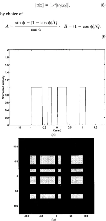
Fig. 3. Input function1a2 cross section and 1b2 two-dimensional, separable function obtained with a pair of different one-dimen-sional functions in outer-product form.

Fig. 2. Setup for performing the fixed-scale asymmetrical FRT. Fig. 1. Setup for performing a two-dimensional fractional Fourier

transform according to the WDF definition.

A convenient selection for Q is Q 5 1, which implies f 5 f1.

To acquaint ourselves with the FRT operator, we performed computer simulations. Based on the above two definitions, two approaches were suggested: one is based on the HG definition3Eq. 1224, and the second is based on the WDF definition 3Eq. 1524. Eq. 152 suggests the performance of a Fourier transformation on the input function multiplied by a quadratic phase term 1chirp term2. Because of the high frequencies necessary to represent truly the chirp term, the resolution necessary to represent the quadratic phase term is much higher than that of the input, requiring a high number of sampling points.

The other FRT computer-implementation approach is based on the HG definition. With the modal notation,2_{Eq.122 can be written as}

ua5 Fa3u04 5 CbaC21u0, 1102

where bais a diagonal matrix having exp12ipam@22 as its mth diagonal element, and the C matrix is con-structed from the HG functions Cmas its rows. Each HG function is normalized by1hm21@2_{to ensure that C}

is orthonormal. We found the HG approach to be the faster simulation procedure, and thus it was used here for performing the computer experiments.

AMATLABsubroutine was written based on Eq.1102. First, the HG modes C were calculated and stored as a random-access-memory variable. Now each FRT of a vector consists of the product of the input vector by CbaC21_{. C}21 _{5 C}T_{, and ba is diagonal. Thus} the number of operations is 2N2 _{for the two matrix–}

vector multiplications, whereas ba1C21_u

02 is a vector–

vector multiplication1only N operations2. C is

com-puted only once. Consequently each FRT calculation consist mainly of two matrix–vector multiplications, which are performed relatively fast. For example, the number of operations for a 256-element input vector1N 5 2562 is roughly 2N2_{5 132,000 operations.}

The input vector length is always N; thus the required number of operations is independent of the fractional order.

The experimental demonstration of the FRT was performed with bulk-optics setups, both for the sym-metrical one1Fig. 12 and the asymmetrical one 1Fig. 22. Although the GRIN approach could be useful for laboratory experiments, the superiority of the bulk-optics system is apparent because of its much higher SW1space bandwidth product2 performance and flex-ibility. The GRIN approach did serve for the com-puter simulations.

Figure 3 shows the input function that was used for the simulations and for the experiments. For sym-metrical-set-up laboratory experiments a single lens

with f 5 250 mm was used. The control of the

fractional order was done by a change in the param-eter z; thus, as mentioned above, the scale of the input and the output depends on the FRT order. The input mask size was 3.75 mm. The distance z to obtain different fractional orders a is given by a combination of Eqs.132 and 142:

z 5 f tan f@2 sin f, 1112

where f 5 a1p@22.

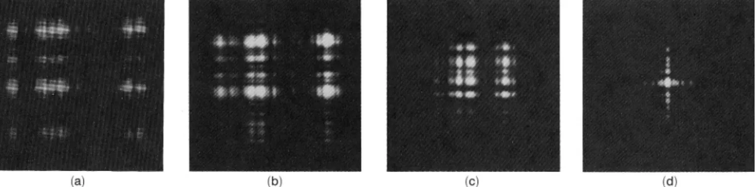
Figures 41a2–41d2 show the experimental results of the intensity distribution for fractional orders a equal to 0.25, 0.5, 0.75, and 1, respectively. The optical setup of Fig. 1 was used with the parameters of Table 1. A fixed lens was used. Thus the various order experiments were done with a different scale factor of Fig. 4. FRT experimental result obtained with the optical symmetrical setup of Fig. 1 with the parameters of Table 1. The FRT order is 1a2 a 5 0.25, 1b2 a 5 0.5, 1c2 a 5 0.75, and 1d2 a 5 1.

Table 1. Parametersa_{Used for Performing the Symmetrical}

Setup Experiments FRT Order a f° R Q f11mm2 Z1mm2 0.25 22.5 0.199 0.383 95.75 19.05 0.50 45 0.414 0.707 176.75 73.17 0.75 67.5 0.668 0.924 231.0 154.31 1 90 1 1 250 250

a_{These parameters take into account different scale factors for}

the various FRT orders.

Table 2. Parametersa_{Used for Performing the Asymmetrical}

Setup Experiments FRT Order a f° Af11mm2 Bf11mm2 0.25 22.5 83.0 19.0 0.50 45 146.5 73.25 0.75 67.5 200.25 154.25 1 90 250 250 a_{f is 250 mm.}

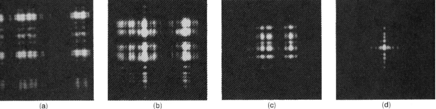
the input and the output. This was taken into account when the computer simulations were per-formed, and an excellent agreement of the experimen-tal and computer-simulation results was obtained. For brevity we omitted the computer-simulation plots. An additional set of experiments was performed in order to explore the asymmetrical configuration. According to Fig. 2, the parameters of the setup were calculated to provide the FRT orders 0.25, 0.5, 0.75, and 1. These parameters are presented in Table 2; f and l are the same as in the symmetrical experiment. Figure 5 shows the obtained results. The results were compared with the computer-simulation results, and again an excellent agreement was obtained.

To conclude, we have introduced the various possi-bilities for implementing the fractional-Fourier-transform operation. For computer simulations the GRIN interpretation was used. A bulk-optics optical implementation was suggested in a configuration very similar to the conventional 2-f Fourier-transform-ing system accordFourier-transform-ing to the WDF interpretation. Two optical setups were introduced, a symmetrical

and an asymmetrical one. It was shown that, with the symmetrical configuration with a fixed lens, the input and the output objects should be scaled. The asymmetrical setup avoids this scale factor but intro-duces a quadratic phase distribution to the output plane. Both setups were implemented optically, and experimental results were demonstrated.

References

1. D. Mendlovic and H. M. Ozaktas, ‘‘Fractional Fourier transfor-mations and their optical implementation. Part I,’’ J. Opt. Soc. Am. A 10, 1875–1881119932.

2. H. M. Ozaktas and D. Mendlovic, ‘‘Fractional Fourier transfor-mations and their optical implementation. Part II,’’ J. Opt. Soc. Am. A 10, 2522–2531119932.

3. A. W. Lohmann, ‘‘Image rotation, Wigner rotation, and the fractional Fourier transform,’’ J. Opt. Soc. Am. A 10, 2181–2186 119932.

4. A. Yariv, Optical Electronics, 3rd ed.1Holt, New York, 19852. 5. D. Mendlovic, H. M. Ozaktas, and A. W. Lohmann,

‘‘Graded-index fibers, Wigner distribution functions, and the fractional Fourier transform,’’ Appl. Opt. 33, 6188–6193119942.

Fig. 5. FRT experimental result obtained with the asymmetrical optical setup of Fig. 2 with the parameters of Table 2. The FRT order is 1a2 a 5 0.25, 1b2 a 5 0.5, 1c2 a 5 0.75 and 1d2 a 5 1.