Effect of Monetary Policy Instruments on Shadow Banking

BUSINESS & MANAGEMENT STUDIES:

AN INTERNATIONAL JOURNAL

Vol.:8 Issue:3 Year:2020, 2531-2545

Citation: Okur, F., & Soylu, Ö.B., Effect of Monetary Policy Instruments on Shadow

Banking, BMIJ, (2020), 8(3): 2531-2545, doi: http://dx.doi.org/10.15295/bmij.v8i3.1442

EFFECT OF MONETARY POLICY INSTRUMENTS ON

SHADOW BANKING

Fatih OKUR 1 _{Received Date (Başvuru Tarihi): 11/03/2020}

Özgür Bayram SOYLU 2 _{Accepted Date (Kabul Tarihi): 9/08/2020}

Published Date (Yayın Tarihi): 25/09/2020 ABSTRACT Keywords: Monetary Policy, Shadow Banking, Panel ARDL JEL Codes:

E40, E44, E52, G23

Shadow banks are financial mediators. There are maturity, credit, and liquidity transformation without access to central bank liquidity and public sector credit guarantees in their performance. The principle purpose of this study is to answer the question of the relationship between shadow banking and monetary policy, all financial activities that require a private or public payment guarantee other than traditional banking. This study analyses the short and long-term effects of national income, policy rate, CPI and money supply (M1) on shadow banking by using Panel ARDL method in selected ten countries throughout 2002-2016. The findings of the analysis point out that there is a short- and significant long-term relationship between the indicators discussed. Short-term PMG estimation results indicate that the long-term equilibrium will be reached over for approximately four years. Also, long-term PMG estimation results also pointed to the existence of a significant relationship between indicators, apart from national income. It is determined that the money supply and policy interest rate had a positive relation and the consumer price index had a negative relation with shadow banking.

PARA POLİTİKASI ARAÇLARININ GÖLGE BANKACILIK ÜZERİNDEKİ ETKİSİ ÖZ Anahtar Kelimeler: Para Politikası, Gölge Bankacılık, Panel ARDL JEL Kodları:

E40, E44, E52, G23

Gölge bankalar finansal aracılardır. İşlemlerini merkez bankası likiditesine ve kamu kesimi kredi teminatlarına erişim olmaksızın vade, kredi ve likidite dönüşümü olarak yapmaktadır. Bu çalışmanın temel amacı, gölge bankacılık ve para politikası arasındaki ilişki sorununa, geleneksel bankacılık dışında özel veya kamu ödeme garantisi gerektiren tüm finansal faaliyetlerin yanıtlanmasıdır. Bu çalışmada 2002-2016 döneminde OECD ve OECD ile yakın işbirliğinde olan anahtar konumundaki ülkelerde milli gelir, politika faizi, tüketici fiyat endeksi ve para arzının (M1) gölge bankacılık üzerindeki kısa ve uzun dönemli etkileri yıllık verilerle Panel ARDL yöntemi aracılığıyla tahmin edilmiştir. Analiz sonuçları ele alınan göstergeler arasında kısa ve uzun dönemli anlamlı bir ilişkinin varlığına işaret etmektedir. Kısa vadeli PMG tahmin sonuçları uzun dönem dengesine yaklaşık dört yıllık bir süre zarfında varılacağına işaret etmektedir. Ayrıca uzun dönem PMG tahmin sonuçları da göstergeler arasında milli gelir dışında anlamlı bir ilişkinin varlığına işaret etmiştir. Para arzı ve politika faiz oranın pozitif, tüketici fiyat endeksinin ise negatif bir etkisinin olduğu görülmüştür.

1_{Dr. Öğr.Üyesi, Bayburt Üniversitesi İİBF İktisat Bölümü, fatih.okr@bayburt.edu.tr, https://orcid.org/0000-0002-4686-4563} 2_{Dr. Öğr. Üyesi, Kocaeli Üniversitesi İİBF İktisat Bölümü, ozgurbayram.soylu@kocaeli.edu.tr, https://orcid.org/0000-0002-5030-5924}

1. INTRODUCTION

Shadow banking is not a new term. There are some different definitions. The Financial Stability Board describes shadow banking as credit institutions that conduct activities out of traditional bank systems in general. In McCulley's speech, he stated that shadow banking institutions focused on the US and that shadow banking institutions are predominantly non-bank institutions that were involved in maturity transformation. Pozsan et al. (2012) make a definition of shadow banking. Shadow banks are financial mediators. There are maturity, credit, and liquidity transformation without access to central bank liquidity and public sector credit guarantees in their performance. Claessens et al. (2014) describe shadow banking as all financial activities that require a private or public payment guarantee other than traditional banking.

While unique payment guarantees usually come as the franchise value of another financial institution, public payment guarantees tend to provide guarantees for debt securities and deposit insurance (Elliott et al., 2015). Shadow banks perform similar functions with traditional banks and assume the same risks. Shadow banks perform under different and fewer regulatory supervisions. These features increase the risks that bring financial stability. For this reason, shadow banks are given attention nowadays (Elliott et al., 2015). Shadow banking symbolises one of the many financial failures that have caused a worldwide crisis. When commercial banks use deposits for long-term loan funds, they are involved in maturity transformation. Shadow banks do similar things. Shadow banks increase short-term funds and use them to purchase long-term assets (Kodres, 2013).

Shadow banking includes credit, liquidity and maturity transformation risks, just like traditional banking. That is accepted by the current literature and overlaps with all shadow banking activities. While traditional banking is now safe and stable, the shadow banking system is not secure due to the private sector's liquidity and loans (Pozsar et al., 2010). The extensive feature of nontraditional activities is that generate wages and non-interest income for banks. Therefore, the most likely option for measuring nontraditional activities is non-interest income which is less than the deposit revenues. The measurement of nontraditional activities is referred to as net

non-interest income at this point. Deposit service fees are excluded from traditional banking activities as they are part of traditional banking rather than nontraditional banking (Rogers, 1998).

Because of cheaper service, shadow banks can contribute to economic growth. However, there is always a trade-off situation in terms of lower financial stability. There is a trade-off because of the flexibility of shadow banks, and price competitiveness often brings a safety share cost (Elliott et al., 2015).

There are significant economic benefits and costs. On the benefit side, shadow banks are helping financial growth. They can trade at lower costs than traditional banking and therefore supply cheap loans and other financial services. They can also offer financial services that traditional banks cannot or cannot do (Elliott et al. , 2015). The 2008-2009 financial crisis is a crisis that works from shadow banks across the system. Because it is not in the traditional banking system, but the shadow banking system. While bank runs occur in the traditional banking system as withdrawal of deposits, it occurs as cancellation of the repurchase agreements in the shadow banking system (Gorton and Metrick, 2012). The essential purpose of this study is to answer the question of the relationship between shadow banking and monetary policy. Understanding the relationship between shadow banking and monetary policy is very important for the monetary policy authorities to form healthier monetary policies, and it is believed that the results and the policy recommendations pointed out in the study will contribute to this policy-making process.

The essential purpose of this study is to answer the question of how and in which direction the selected monetary policy instruments affect shadow banking. Understanding this effect is very important for monetary policy authorities to form healthier monetary policies.

The partitioning of the study is as follows: In the introduction part, shadow banking is emphasised. This section seeks to answer questions such as what shadow banking is, when, and how it emerged. After the introduction, empirical studies on shadow banking are compiled in the literature section. After the literature review, the data and the method used in the study are explained. Moreover, in this section,

empirical findings are included. In the last part of the study, the findings of the results are presented. Besides, policy suggestions are also included in this section.

2. LITERATURE REVIEW

This section examines monetary policy and empirical studies on shadow banking. The literature has been examined chronologically in terms of methods applied within itself.

Long et al. (2013) analysed the interest rate effect on shadow banking. Empirical findings show that the rise in interest rate will affect shadow banking in the long-run. Haisen and Yazdifar (2015) used the SVAR model to see if there is shadow banking effect on monetary policy. SVAR model includes variables such as total loans, GDP, CPI, short-term interest rate and money supply (M1). Empirical findings show that if there is an increase in the shadow banking system, monetary policy will be affected by increasing the money supply and the value of CPI.

Nelson et al. (2016) used a VAR model for the USA to analyse monetary policy and shadow banking. The VAR model includes variables such as GDP, CPI, market interest rate and total financial assets. Empirical results show that a contractionary monetary policy negatively affects commercial bank assets, but assets of shadow banks increase.

Gabrieli et al. (2017) used the VECM method to analyse the shadow banking system and monetary policy in China. Findings show that Shadow Banking weakens the effects of interest rate on monetary policy decisions.

Hussain et al. (2019) used the GEE method to analyse the relationship between the shadow banking system and the real economy. According to the findings, if SBS increases, nominal GDP increases rather than real GDP. Lu and Lau (2019) analysed shadow banking in China, monetary policy and macro variables. Empirical results show that money supply and GDP affect on the scale of shadow banking.

Nelson et al. (2015), Jianjun and Xun (2016) used the VAR method in their study to investigate the effect of shadow banking on the monetary transmission mechanism.

It is concluded that shadow banking negatively affected the monetary transmission mechanism.

Altunbas et al. (2009), Lopreite (2012), Xiao (2016) analysed the relationship between shadow banking and monetary policy transmission mechanism. GMM method was used in the study. The GMM model includes variables such as total loans, GDP, M1, interest rate, bank characteristics (size, liquidity, capital). As a result of the empirical tests, it is observed that the effect of monetary policy on economic activities is narrowed when shadow banks are taken into consideration.

According to the literature review on shadow banking, there are many studies in terms of samples and periods. It is observed that more than one econometric model is used in the literature. The majority of studies suggest that shadow banking reduces the monetary policy's impact on the real economy.

3. DATA AND METHODOLOGY 3.1. Data

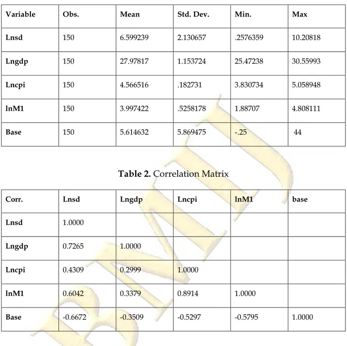
The short and long-term effects of national income, policy rate, CPI and money supply (M1) on shadow banking were estimated by using Panel ARDL method in critical countries in close cooperation with OECD and OECD in 2002-2016 period in this study. Annual data is obtained from the World Bank, IMF, OECD databases and countries' central bank data. The reason for starting the operating range from 2002 is that the shadow banking data exists from the relevant year. The countries covered in the study are Australia, Brazil, Canada, China, Mexico, South Africa, Switzerland, Turkey, Britain and the United States. Although Brazil, China and South Africa are not OECD countries, they are in close cooperation with the OECD. While Table 1 contains descriptive statistics for the variables used in the study, Table 2 represents the correlation matrix for these variables.

Table 1. Descriptive Statistics

Variable Obs. Mean Std. Dev. Min. Max

Lnsd 150 6.599239 2.130657 .2576359 10.20818

Lngdp 150 27.97817 1.153724 25.47238 30.55993

Lncpi 150 4.566516 .182731 3.830734 5.058948

lnM1 150 3.997422 .5258178 1.88707 4.808111

Base 150 5.614632 5.869475 -.25 44

Table 2. Correlation Matrix

Corr. Lnsd Lngdp Lncpi lnM1 base

Lnsd 1.0000

Lngdp 0.7265 1.0000

Lncpi 0.4309 0.2999 1.0000

lnM1 0.6042 0.3379 0.8914 1.0000

Base -0.6672 -0.3509 -0.5297 -0.5795 1.0000

Among the variables, lnsd; logarithm of shadow banking data, lngdp; logarithm of the national income level at current prices, lncpi; the logarithm of the consumer price index, lnM1; the money represents the logarithm. The base represents the policy interest rate. Stata and Eviews programs are used for an empirical application.

3.2. Methodology

Panel unit root tests are examined under two generations according to whether there is a correlation between units. It is essential to test the existence of a correlation between units before applying a unit root test in this respect. Several tests have been

developed to test the inter-unit correlation. The most appropriate test for asymptotic properties data set should be preferred by testing the correlation between units.

It is typically assumed that disturbances in panel data models are cross-sectional independent (Peseran 2004). The countries of the panel, the units of horizontal sections are independent based on the assumption that all horizontal cross-sectional units are affected at the same level and that no other countries are affected by a macroeconomic shock in any of the countries. It is necessary to test whether there is a cross-section dependency between the series before starting the analysis. The results obtained in the analysis without considering the cross-section dependency will be perverted and inconsistent. Three tests are generally used to test the cross-sectional dependence in panel data analysis. Breusch-Pagan (1980) argues that the cross-sectional dependence is valid when N is constant, and T goes to infinity (T → ∞). That is, T> N. Breusch-Pagan's (1980) cross-sectional dependence test is developed under the "No cross-sectional dependency" null hypothesis. It is calculated by the equation below.

𝐶𝐶𝐶𝐶𝐵𝐵𝐵𝐵= 𝑇𝑇 ∑𝑁𝑁−1𝑡𝑡=1 ∑𝑁𝑁𝑗𝑗=𝑖𝑖+1ῤ𝑡𝑡,𝑗𝑗2 (1)

The second cross-sectional dependence test is the CDLM test developed by Pesaran (2004). This test is valid if T and N are large (N → ∞ and T→∞)). The test has standard normal distribution under the null hypothesis "no cross-sectional dependency" and calculated as follows:

𝐶𝐶𝐶𝐶𝐿𝐿𝐿𝐿1= �1/𝑁𝑁(𝑁𝑁 − 1) ∑𝑁𝑁−1𝑡𝑡=1 ∑𝑁𝑁𝑗𝑗=𝑖𝑖+1(𝑇𝑇ῤ𝑡𝑡,𝑗𝑗2 − 1) (2)

The CDLM test developed by Pesaran (2004), one of the cross-sectional dependence tests, has a standard normal distribution under the null hypothesis "No cross-sectional dependency". This test is valid when T is constant, and N is infinity (N → ∞). In other words, it is valid when N>T and calculated as follows:

𝐶𝐶𝐶𝐶𝐿𝐿𝐿𝐿 = �2𝑇𝑇/𝑁𝑁(𝑁𝑁 − 1) (∑𝑁𝑁−1𝑡𝑡=1 ∑𝑁𝑁𝑗𝑗=𝑖𝑖+1ῤ𝑖𝑖,𝑗𝑗 (3)

Another cross-sectional dependence test is LMadj (bias-adjusted) which was performed by Pesaran et al. (2008). μTij and νTij are the mean and variance of (T − k)

ρ̂ij2 proposed by Pesaran et al. (2008). LMadj exhibits normal asymptotic standard distribution while T → ∞ and N →∞ under the null hypothesis that there is no horizontal cross-section dependence. Breusch and Pagan (1980) LM test and Pesaran et al. (2008) (bias-adjusted) LM test are applied since T is larger N (T>N).

𝐿𝐿𝐿𝐿𝑎𝑎𝑎𝑎𝑗𝑗 = �2/𝑁𝑁(𝑁𝑁 − 1) (∑𝑁𝑁−1𝑖𝑖=1 ∑𝑁𝑁𝑗𝑗=𝑖𝑖+1𝑇𝑇ῤ𝑖𝑖,𝑗𝑗(𝑇𝑇−𝑘𝑘)ῤ𝑖𝑖𝑖𝑖

2_{− µ} 𝑇𝑇𝑖𝑖𝑖𝑖

�ὐ𝑇𝑇𝑖𝑖𝑖𝑖2

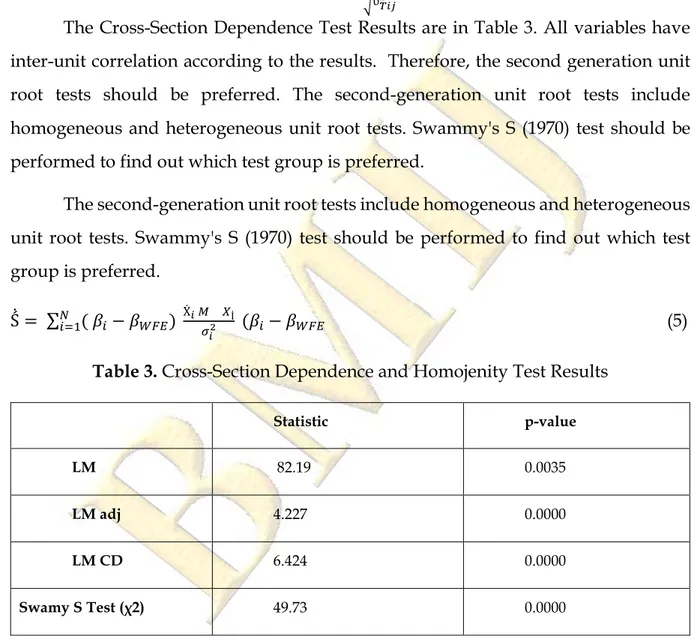
(4) The Cross-Section Dependence Test Results are in Table 3. All variables have inter-unit correlation according to the results. Therefore, the second generation unit root tests should be preferred. The second-generation unit root tests include homogeneous and heterogeneous unit root tests. Swammy's S (1970) test should be performed to find out which test group is preferred.

The second-generation unit root tests include homogeneous and heterogeneous unit root tests. Swammy's S (1970) test should be performed to find out which test group is preferred.

Ṥ = ∑ ( 𝛽𝛽𝑁𝑁𝑖𝑖=1 𝑖𝑖 − 𝛽𝛽𝑊𝑊𝑊𝑊𝑊𝑊) Ẋ𝑖𝑖 𝐿𝐿 𝑋𝑋_𝜎𝜎 İ

𝑖𝑖2 (𝛽𝛽𝑖𝑖 − 𝛽𝛽𝑊𝑊𝑊𝑊𝑊𝑊 (5)

Table 3. Cross-Section Dependence and Homojenity Test Results

Statistic p-value

LM 82.19 0.0035

LM adj 4.227 0.0000

LM CD 6.424 0.0000

Swamy S Test (χ2) 49.73 0.0000

More recently, Pesaran and Yamagata (2008) suggest a dispersion type test based on Swamy (1970) type test. They standardise the Swamy type test so that the test can be applied when both n and T are large. The Swamy S Test Results are in Table 3.

The Swamy Test results indicate that the series are heterogeneous because the probability value is less than 0.05. Horizontal section dependency test results require the rejection of the H0 hypothesis "there is no horizontal section dependency between the series". The heterogeneity of the series and the presence of horizontal cross-section depend on the application of second-generation tests from unit root tests.

3.2.1. Unit Root Test

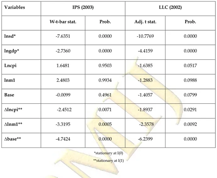
Im, Pesaran and Shin (IPS, 2003), and Levin, Lin and Chu (LLC, 2002) unit root tests are used to determine the stationary of the data in the panel. LLC panel unit root test is among the first group PUR test, while the IPS included in the second group PUR test. The main difference between the first group PUR tests and the second group PUR is the application of unit root separately to the time series of all units in the second group tests and the units owning their autoregressive parameters (Tatoğlu, 2018; 41).

The first and second group PUR test regarding the variables used in the study gives similar results. In both unit root tests, Ho hypothesis established as "contains unit root for all units". Table 4 shows the unit root test results for the variables used in the study.

Table 4. Unit Root Test Results

Variables IPS (2003) LLC (2002)

W-t-bar stat. Prob. Adj. t stat. Prob.

lnsd* -7.6351 0.0000 -10.7769 0.0000 lngdp* -2.7360 0.0000 -4.4159 0.0000 Lncpi 1.6481 0.9503 -1.6385 0.0517 lnm1 2.4803 0.9934 -1.2883 0.0988 Base -0.0099 0.4961 -1.4057 0.0799 ∆lncpi** -2.4512 0.0071 -1.8937 0.0291 ∆lnm1** -3.3195 0.0005 -2.3578 0.0092 ∆base** -4.7424 0.0000 -6.2399 0.0000 *stationary at I(0) **stationary at I(1)

The unit root test results indicate that the shadow banking and national income series are stationary at the level. Besides, the consumer price index, money supply and policy interest rates are stationary at first differences.

3.2.2. Hausman Test and Pooled Group Estimator

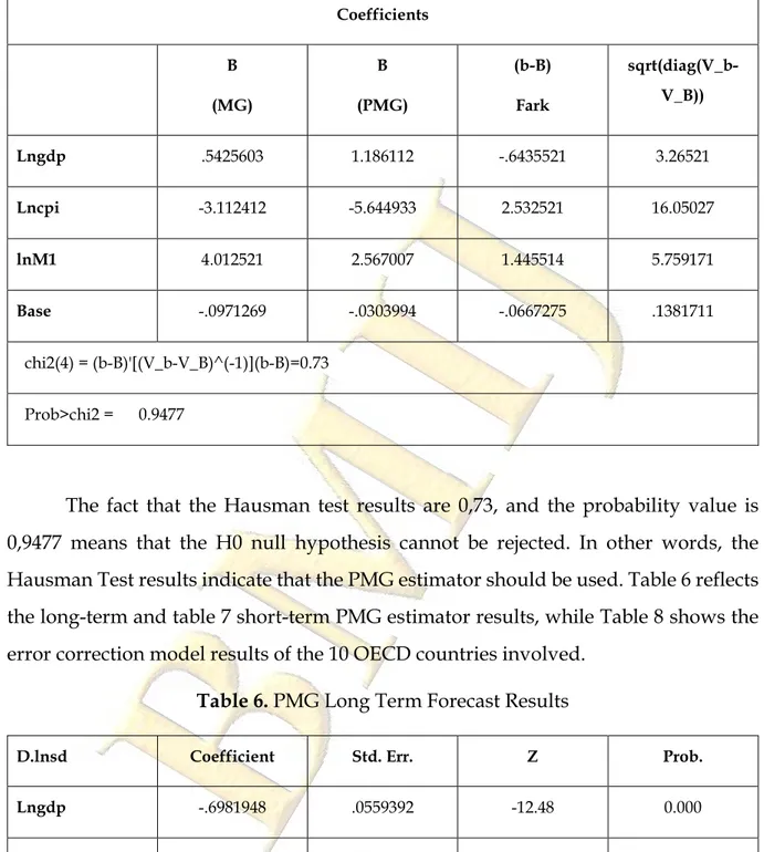
Before making long and short term estimates, it is necessary to determine whether the Mean Group (MG) estimator or the Pooled Group (PMG) estimator is used. Hausman test is used to make this decision. Table 5 reflects the Hausman test results.

Table 5. Hausman Test Results Coefficients B (MG) B (PMG) (b-B) Fark sqrt(diag(V_b-V_B)) Lngdp .5425603 1.186112 -.6435521 3.26521 Lncpi -3.112412 -5.644933 2.532521 16.05027 lnM1 4.012521 2.567007 1.445514 5.759171 Base -.0971269 -.0303994 -.0667275 .1381711 chi2(4) = (b-B)'[(V_b-V_B)^(-1)](b-B)=0.73 Prob>chi2 = 0.9477

The fact that the Hausman test results are 0,73, and the probability value is 0,9477 means that the H0 null hypothesis cannot be rejected. In other words, the Hausman Test results indicate that the PMG estimator should be used. Table 6 reflects the long-term and table 7 short-term PMG estimator results, while Table 8 shows the error correction model results of the 10 OECD countries involved.

Table 6. PMG Long Term Forecast Results

D.lnsd Coefficient Std. Err. Z Prob.

Lngdp -.6981948 .0559392 -12.48 0.000

Lncpi -1.510797 .3954279 -3.82 0.000

lnM1 .129204 .0858427 1.51 0.132

Base .0456744 .0113876 4.01 0.000

Long term forecasting results show that variables examined in the long term have a significant relationship with the shadow banking variable, except for money

supply. For example, a 1% change in national income has a negative impact of 0.69% on shadow banking in the long run. Similarly, the 1% change in the consumer price index has a negative impact of 1.51% on shadow banking in the long run. Money supply and policy interest rate, on the other hand, have a positive effect on the 10 OECD countries examined.

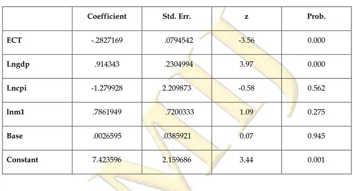
Table 7. PMG Short Term Forecast Results

Coefficient Std. Err. z Prob.

ECT -.2827169 .0794542 -3.56 0.000 Lngdp .914343 .2304994 3.97 0.000 Lncpi -1.279928 2.209873 -0.58 0.562 lnm1 .7861949 .7200333 1.09 0.275 Base .0026595 .0385921 0.07 0.945 Constant 7.423596 2.159686 3.44 0.001

It is determined that the error correction coefficient is calculated as -.28, the sign of the coefficient is negative as expected, and the probability value is less than 0.05 and significant. It points out that any shock to the shadow banking series will converge to a long-term equilibrium in about four years, with a convergence of 28% each year to stabilise in the long term.

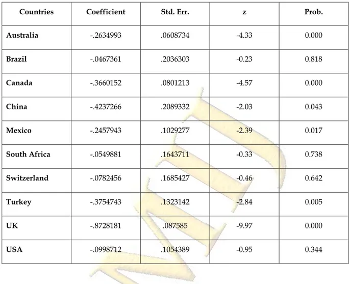
Table 8. Error Correction Coefficient (ECT) by Countries

Countries Coefficient Std. Err. z Prob.

Australia -.2634993 .0608734 -4.33 0.000 Brazil -.0467361 .2036303 -0.23 0.818 Canada -.3660152 .0801213 -4.57 0.000 China -.4237266 .2089332 -2.03 0.043 Mexico -.2457943 .1029277 -2.39 0.017 South Africa -.0549881 .1643711 -0.33 0.738 Switzerland -.0782456 .1685427 -0.46 0.642 Turkey -.3754743 .1323142 -2.84 0.005 UK -.8728181 .087585 -9.97 0.000 USA -.0998712 .1054389 -0.95 0.344

The error correction coefficients are negative and significant in six countries other than the USA, Switzerland, South Africa and Brazil. It is seen that the country showing the fastest convergence to the long-term balance in the UK and the country showing the slowest convergence is Mexico.

4. CONCLUSION

In this study, a long and short-term relationship between the shadow banking indicator and the national income, consumer price index, money supply and policy interest rate, with a panel data study of 10 countries is investigated from 2002 to 2016. The results of the analysis point out that there is a short and long term significant relationship between the indicators discussed. The short-term PMG estimation results indicate that the long-term equilibrium will be reached over approximately four years.

Also, long-term PMG estimation results pointed to the existence of a meaningful relationship between indicators except for national income. It was

determined that the money supply and policy interest rate had a positive effect and the consumer price index had a negative impact. Although the coefficient of the national income indicator has a positive sign that is compatible with the literature, it does not have a significant relationship. The results of error correction terms examined by countries indicate that the convergence rate varies from 24% to 87% by countries. The growth of the shadow credit market in the world is still under development. Regulatory authorities should maintain an objective attitude towards the growth of the shadow credit market, improve the regulatory environment and strengthen control. For the effective allocation of resources, the effects of the shadow banking system on economic growth and money supply should be taken into account.

REFERENCES

Adrian, T., Ashcraft, A., Boesky, H., & Pozsar, Z. (2012). Shadow banking. Revue d'économie financière, (1), 157-184.

Altunbas, Y., Gambacorta, L., ve Marques-Ibanez, D. (2009). Securitisation and the bank lending channel. European Economic Review, 53(8), 996-1009.

Claessens, S., & Ratnovski, L. (2014). What Is Shadow Banking? IMF Working Paper. WP/14/25. IMF. Research Department.

Elliott, D., Kroeber, A., ve Qiao, Y. (2015). Shadow banking in China: A primer. Research paper, The Brookings Institution.

Gabrieli, T., Pilbeam, K., & Shi, B. (2018). The impact of shadow banking on the implementation of Chinese monetary policy. International Economics and Economic Policy, 15(2), 429-447.

Gorton, G., ve Metrick, A. (2012). Securitised banking and the run on repo. Journal of Financial economics, 104(3), 425-451.

Hussain, A., & Bao, J. (2019). The impacts of Shadow banking system on economy. An empirical analysis. Journal of Applied Finance and Banking, 9(3), 1-11.

Im, K. S., Pesaran, M. H., & Shin, Y. (2003). Testing for unit roots in heterogeneous panels. Journal of econometrics, 115(1), 53-74.

Jianjun, L., ve Xun, H. (2016). The Macroeconomic Effect of Shadow Credit Market Financing. Applied Economics and Finance, 3(3), 158-171.

Kodres, L. E. (2013). What is shadow banking. Finance and Development, 50(2), 42-43.

Levin, A., Lin, C. F., & Chu, C. S. J. (2002). Unit root tests in panel data: asymptotic and finite-sample properties. Journal of econometrics, 108(1), 1-24.

Long, J. C., FAN, X. J., & ZHANG, X. (2013). Changes in Interest Rate, Shadow Banking and SME Financing. In Finance Forum (Vol. 7).

Lopreite, M. (2012). Securitisation and monetary transmission mechanism: evidence from italy (1999-2009).

Lu, T., & Lau, W. Y. (2019). China's Shadow Banking: Dynamics of Policy and Economy. In Finance and Strategy Inside China (pp. 131-146). Springer, Singapore.

Nelson, B. D., Pinter, G., ve Theodoridis, K. (2015). Do contractionary monetary policy shocks expand shadow banking? Bank of England Working Paper No. 521

Pedroni, P. (2004). Panel cointegration: asymptotic and finite sample properties of pooled time series tests with an application to the PPP hypothesis. Econometric theory, 20(3), 597-625.

Pozsar, Z., Adrian, T., Ashcraft, A. B., ve Boesky, H. (2010). Shadow banking. Staff Report no. 458 Rogers, K. E. (1998). Nontraditional activities and the efficiency of US commercial banks. Journal of Banking ve Finance, 22(4), 467-482.

Tatoğlu, F. Y. (2018). İleri panel veri analizi: Stata uygulamalı. Beta Xiao, K. (2016). How Does Monetary Policy Affect Shadow Bank Money.