Asymptotic and numerical methods in estimating eigenvalues

(1)

Volume 2013, Article ID 415479,8pages http://dx.doi.org/10.1155/2013/415479

Research Article

Asymptotic and Numerical Methods in Estimating Eigenvalues

Guldem Y

JldJz,

1

Bulent Y

Jlmaz,

2

and O. A. Veliev

3

1_{Department of Mathematics, Nigde University, 51200 Nigde, Turkey}

2_{Department of Math, Faculty of Science and Letters, Marmara University, Göztepe Kampüsü, Kadiköy, 81040 Istanbul, Turkey} 3_{Department of Mathematics, Dogus University, Acıbadem, Kadiköy, 81010 Istanbul, Turkey}

Correspondence should be addressed to Guldem Yıldız; guldem.yildiz@nigde.edu.tr Received 17 January 2013; Accepted 8 March 2013

Academic Editor: Safa Bozkurt Coskun

Copyright © 2013 Guldem Yıldız et al. This is an open access article distributed under the Creative Commons Attribution License, which permits unrestricted use, distribution, and reproduction in any medium, provided the original work is properly cited. Asymptotic formulas and numerical estimations for eigenvalues of SturmLiouville problems having singular potential functions, with Dirichlet boundary conditions, are obtained. This study gives a comparison between the eigenvalues obtained by the asymptotic and the numerical methods.

1. Introduction

Let𝐿(𝑞) be an operator generated in 𝐿₂[0, 1] by the expres-sion

𝐿 (𝑞) = −𝑦󸀠󸀠(𝑥) + 𝑞 (𝑥) 𝑦 (𝑥) , 0 ≤ 𝑥 ≤ 1, (1) and by Dirichlet boundary conditions

𝑦 (0) = 𝑦 (1) = 0, (2)

where𝑞(𝑥) is a complex-valued summable function. In this paper, we consider the small and large eigenvalues of the operator 𝐿(𝑞) when 𝑞(𝑥) has a finite number of singularities. The large eigenvalues are investigated by the asymptotic method given in [1, 2]. Note that in classical investigations in order to obtain the asymptotic formulas of order𝑂(𝑛−𝑙) it is required that 𝑞(𝑥) be (𝑙 − 1) times differen-tiable (see [3–10]). The method of [1] gives the possibility of obtaining the asymptotic formulas of order𝑂(𝑛−𝑙) of eigen-values and eigenfunctions of𝐿(𝑞) when 𝑞(𝑥) is an arbitrary summable complex-valued function. The small eigenvalues are investigated by numerical and asymptotic methods. Then, we compare the results with the ones obtained by the other methods.

Expression of differential equations in matrix form and the advances in the field of the computers have led to major developments in numerical methods. Regarding the

numerical solution of the Sturm-Liouville problems, finite difference method is amongst the popular methods (see [11,

12]). Finite difference method can give effective results for the eigenvalues when it is used in connection with asymptotic correction technique. In [13] and [14] the Sturm-Liouville problems with Dirichlet and the general boundary conditions were studied, respectively. Andrew and Paine [15] found the approximate eigenvalues of regular Sturm-Liouville problem by using the finite element method. Chen and Ho [16] used the differential transform method to solve the eigenvalue problems. Ghelardoni [17] named some linear multistep methods as boundary value methods and found the approx-imate eigenvalues of Sturm-Liouville problem. Ghelardoni and Gheri [18] used the shooting technique for the calculation of the eigenvalues of Sturm-Liouville problem by considering the Pr¨ufer transformation given in [19]. Kumar [20], Kumar and Aziz [21] gave numerical examples to linear or nonlinear boundary value problems by using finite differences method for singular boundary value problems. Kumar and Singh [22] made a study which collected and classified various calculation techniques for the solution of singular boundary value problems.

2. Asymptotic Formulas for Eigenvalues

It is well known that (see formulas (47a), (47b) in page 65 of [7]) the eigenvalues of the operator 𝐿(𝑞), where 𝑞(𝑥) is

(2)

a complex-valued summable function, consist of the sequence{𝜆_𝑛} satisfying

𝜆_𝑛= (𝑛𝜋)2+ 𝑂 (1) . (3)

In [1] (see Theorem 1 of [1]), it is proved that the eigenvalues𝜆_𝑛satisfy the following formula

𝜆_𝑛= (𝑛𝜋)2+ 𝐶₀+ 𝐹_𝑚+ 𝑂 ((ln_𝑛|𝑛|)𝑚+1) , ∀𝑚 = 0, 1, 2, . . . , (4) where𝐹₀= −𝐶_2𝑛, 𝐶_𝑛= ∫₀1𝑞(𝑥) cos 𝑛𝜋𝑥 𝑑𝑥, 𝐹₁= 𝐴₁((𝑛𝜋)2) = −𝐶_2𝑛+ ∑∞ 𝑛1=−∞ 𝑛1 ̸= −2𝑛 𝐶_𝑛1(𝐶_𝑛1− 𝐶_𝑛1+2𝑛) [(𝑛𝜋)2_{− (𝜋 (𝑛 + 𝑛} 1))2] , (5) 𝐹𝑘= 𝐴𝑘((𝑛𝜋)2+ 𝐹𝑘−1) , ∀𝑘 = 2, 3, . . . . (6)

Note that in [1], without loss of generality, it was assumed that 𝐶₀ = 0. Then using (4), the cases𝑞(𝑥) = 𝑝(𝑥) + 𝑐/𝑥𝛼 and 𝑞(𝑥) = 𝑎₀/√𝑥 + 𝑎₁/√1 − 𝑥 + 𝑏₀√𝑥 + 𝑏1√1 − 𝑥 (where 𝑐 , 𝑎0,

𝑎₁, 𝑏₀, 𝑏₁are complex numbers) are investigated in detail. In this paper, we consider the case

𝑞 (𝑥) =∑]

𝑘=0

𝑐_𝑘 󵄨󵄨󵄨󵄨𝑥 − 𝑡𝑘󵄨󵄨󵄨󵄨𝛼𝑘

, 0 < 𝛼_𝑘< 1, (7) where] is a positive integer and 𝑐_𝑘is a complex number. First using (4) we prove the following.

Theorem 1. The eigenvalue 𝜆_𝑛 of the operator 𝐿(𝑞) with

potential (7) satisfies the asymptotic formula:

𝜆𝑛 = (𝑛𝜋)2+ 𝐶0 −∑] 𝑘=0 𝑐_𝑘 (2𝑛)1−𝛼𝑘(cos 2𝑛𝜋𝑡𝑘(𝑑4𝑘+ 𝑑4𝑘+2) − sin 2𝑛𝜋𝑡_𝑘(𝑑_4𝑘+1+ 𝑑_4𝑘+3)) + 𝑂 (ln|𝑛| 𝑛 ) , (8) where 𝑑_4𝑘 = ∫∞ 0 cos𝜋𝑠 𝑠𝛼𝑘 𝑑𝑠, 𝑑4𝑘+2= ∫ 0 −∞ cos𝜋𝑠 𝑠𝛼𝑘 𝑑𝑠, 𝑑_4𝑘+1= ∫0 −∞ sin𝜋𝑠 𝑠𝛼𝑘 𝑑𝑠, 𝑑4𝑘+3= ∫ ∞ 0 sin𝜋𝑠 𝑠𝛼𝑘 𝑑𝑠. (9)

Proof. At (4) for𝑚 = 0, let us use the formula

𝜆𝑛= (𝜋𝑛)2+ 𝐶0− 𝐶2𝑛+ 𝑂 (ln_𝑛|𝑛|) , (10) where 𝐶_𝑛= ∫1 0 𝑞 (𝑥) cos 𝑛𝜋𝑥 𝑑𝑥 = ] ∑ 𝑘=0 ∫1 0 𝑐_𝑘cos𝑛𝜋𝑥 (𝑥 − 𝑡_𝑘)𝛼𝑘𝑑𝑥. (11) In the last equality, using the transformations𝑡 = 𝑥 − 𝑡_𝑘and 𝑛𝑡 = 𝑠 we obtain 𝐶𝑛 = ] ∑ 𝑘=0 ∫1−𝑡𝑘 −𝑡𝑘 𝑐_𝑘cos𝑛𝜋 (𝑡 + 𝑡_𝑘) 𝑡𝛼𝑘 𝑘 𝑑𝑡 =∑] 𝑘=0 ∫1−𝑡𝑘 −𝑡𝑘 𝑐_𝑘cos𝑛𝜋𝑡 cos 𝑛𝜋𝑡_𝑘 𝑡𝛼𝑘_𝑘 𝑑𝑡 −∑] 𝑘=0 ∫1−𝑡𝑘 −𝑡𝑘 𝑐_𝑘sin𝑛𝜋𝑡 sin 𝑛𝜋𝑡_𝑘 𝑡𝛼𝑘_𝑘 𝑑𝑡, 𝐶_𝑛 =∑] 𝑘=0 𝑐_𝑘 𝑛1−𝛼𝑘 (cos 𝑛𝜋𝑡𝑘∫ 𝑛(1−𝑡𝑘) −𝑛𝑡𝑘 cos𝜋𝑠 𝑠𝛼𝑘 𝑑𝑠 − sin 𝑛𝜋𝑡_𝑘∫𝑛(1−𝑡𝑘) −𝑛𝑡𝑘 sin𝜋𝑠 𝑠𝛼𝑘 𝑑𝑠) . (12) Let𝑛(1 − 𝑡_𝑘) = 𝑛_𝑘. By (9) we have 𝐶_𝑛=∑] 𝑘=0 𝑐𝑘 𝑛1−𝛼𝑘(cos 𝑛𝜋𝑡𝑘(𝑑4𝑘− ∫ ∞ 𝑛𝑘 cos𝜋𝑠 𝑠𝛼𝑘 𝑑𝑠 +𝑑_4𝑘+2− ∫−𝑛𝑡𝑘 −∞ cos𝜋𝑠 𝑠𝛼𝑘 𝑑𝑠) − sin 𝑛𝜋𝑡_𝑘(𝑑_4𝑘+1− ∫−𝑛𝑡𝑘 −∞ sin𝜋𝑠 𝑠𝛼𝑘 𝑑𝑠 +𝑑_4𝑘+3− ∫∞ 𝑛𝑘 sin𝜋𝑠 𝑠𝛼𝑘 𝑑𝑠)) . (13)

Arguing as in the proof of(41) of [1] one can readily see that

∫−𝑛𝑡𝑘 −∞ cos𝜋𝑠 𝑠𝛼𝑘 𝑑𝑠 = 𝑂 ( 1 𝑛𝛼𝑘_𝑘 ) , ∫ ∞ 𝑛𝑘 cos𝜋𝑠 𝑠𝛼𝑘 𝑑𝑠 = 𝑂 ( 1 𝑛𝛼𝑘_𝑘 ) , ∫−𝑛𝑡𝑘 −∞ sin𝜋𝑠 𝑠𝛼𝑘 𝑑𝑠 = 𝑂 ( 1 𝑛𝛼𝑘 𝑘 ) , ∫∞ 𝑛𝑘 sin𝜋𝑠 𝑠𝛼𝑘 𝑑𝑠 = 𝑂 ( 1 𝑛𝛼𝑘 𝑘 ) . (14)

(3)

Therefore 𝐶_𝑛=∑] 𝑘=0 𝑐_𝑘 𝑛1−𝛼𝑘 (cos 𝑛𝜋𝑡𝑘(𝑑4𝑘+ 𝑑4𝑘+2) − sin 𝑛𝜋𝑡_𝑘(𝑑_4𝑘+1+ 𝑑_4𝑘+3)) + 𝑂 (1 𝑛) . (15)

Thus (8) follows from (4) for𝑚 = 0. The theorem is proved.

Now assuming that

𝛼₁= 𝛼₂= ⋅ ⋅ ⋅ = 𝛼_]= 1

2 (16)

we obtain more precise asymptotic formula by using more subtle estimations.

Theorem 2. If (16) holds, then the eigenvalue𝜆_𝑛of the

opera-tor𝐿(𝑞) with potential (7) satisfies the asymptotic formula: 𝜆_𝑛= (𝑛𝜋)2+ 𝐶₀− 𝐶_2𝑛+ 𝑂 ((ln|𝑛|

𝑛 )

2

) . (17)

Proof. To prove the theorem we use (4) for𝑚 = 1, (5) and

prove that ∞ ∑ 𝑛1=−∞ 𝑛1 ̸= 0,−2𝑛 𝐶2 𝑛1 𝑛₁(2𝑛 + 𝑛₁) = 𝑂 (( ln|𝑛| 𝑛 ) 2 ) , ∞ ∑ 𝑛1=−∞ 𝑛1 ̸= 0,−2𝑛 𝐶_𝑛1𝐶_𝑛1+2𝑛 𝑛₁(2𝑛 + 𝑛₁) = 𝑂 (( ln|𝑛| 𝑛 ) 2 ) . (18)

In (15), instead of𝑛 and 𝛼_𝑘taking𝑛₁and1/2 we get 𝐶_𝑛1=∑] 𝑘=0 𝑐_𝑘 (𝑛₁)1/2(cos 𝑛1𝜋𝑡𝑘(𝑑4𝑘+ 𝑑4𝑘+2) − sin 𝑛₁𝜋𝑡_𝑘(𝑑_4𝑘+1+ 𝑑_4𝑘+3)) + 𝑂 (1 𝑛₁) . (19)

From (19) one can readily see that there exists a constant𝑟 such that 󵄨󵄨󵄨󵄨 󵄨𝐶𝑛1󵄨󵄨󵄨󵄨󵄨 2 < 𝑟_𝑛1 1 (20)

for𝑛₁ = 1, 2, . . .. Therefore, instead of equation (56) of [1], using (20) and repeating the proof of equation(55) of [1] we get the proof of (18). Thus the proof of the theorem follows from (4), (5), and (18). The theorem is proved.

3. Numerical Approximation

Now, we consider the small eigenvalues of the𝐿(𝑞) operator by a numerical method.

For the finite difference method [11,19] take an equally spaced mesh(𝑚 ⩾ 2)

0 = 𝑥₀< 𝑥₁< ⋅ ⋅ ⋅ < 𝑥_𝑚+1= 1, (21) where

𝑥_𝑗= 𝑗ℎ, ℎ = 1

𝑚 + 1. (22)

Writing𝑦(𝑥_𝑗) as 𝑦_𝑗,𝑞(𝑥_𝑗) as 𝑞_𝑗, and𝑦󸀠󸀠(𝑥_𝑗) as 𝑦_𝑗󸀠󸀠, we use the centered difference approximation

−𝑦_𝑗󸀠󸀠 ≈ −𝑦𝑗−1+ 2𝑦𝑗− 𝑦𝑗+1

ℎ2 . (23)

Substituting in (1) we obtain the approximating scheme −𝑌𝑗−1+ 2𝑌𝑗− 𝑌𝑗+1

ℎ2 + 𝑞𝑗𝑌𝑗 = Λ𝑌𝑗, 𝑗 = 1, 2, . . . , 𝑚. (24)

Incorporating the boundary conditions, we get

𝑌₀= 0, 𝑌_𝑚+1= 0. (25)

This can be written in matrix form as

𝑇𝑌 = Λ𝑌, (26)

where

𝑇 = _ℎ1₂𝐾 + 𝑄∗, (27)

𝑇 is a tridiagonal matrix and

𝑌 = ( 𝑌₁ ⋅ ⋅ ⋅ 𝑌_𝑚 ) , 𝐾 =((₍ ( 2 −1 −1 2 −1 ⋅ ⋅ ⋅ −1 2 −1 −1 2 ) ) ) ) , 𝑄∗ = ( ( 𝑞1 𝑞2 ⋅ ⋅ ⋅ 𝑞_𝑚 ) ) . (28)

The eigenvalues of (1), (2) are approximated by the eigenval-ues of matrix T.

(4)

In the previous section, the asymptotic formulas for eigenvalues of the operator𝐿(𝑞) (1), (2) with the potential (7) are investigated. In this section, we will find the eigenvalues of the operator𝐿(𝑞) by using the finite difference method when 𝑐_𝑘 = 1, 𝛼_𝑘 = 1/2 for 𝑘 = 0, 1, . . . , ], and 𝑡_𝑘 = 𝑘/]. Let us introduce the notation

𝑞𝑘(𝑥) = 1

󵄨󵄨󵄨󵄨𝑥 − 𝑡𝑘󵄨󵄨󵄨󵄨1/2 (29)

and denote the𝑛th eigenvalue of the operator 𝐿(𝑞_𝑘) by 𝜆𝑘_𝑛. The 𝑛th eigenvalue of the operator 𝐿(𝑄_]), where

𝑄_](𝑥) =∑]

𝑘=0

𝑞_𝑘(𝑥) , (30)

is denoted byΛ]_𝑛.

In order to be able to apply the Finite Difference method, the nodes should not coincide with the singular points. Let 𝑚_]= ](𝑚 + 1) and 𝑥_𝑗nodal points be

𝑥_𝑗= 𝑗

𝑚_], 𝑗 = 1, 2, . . . , 𝑚]− 1; 𝑗 ̸= 𝑘 (𝑚 + 1) . (31) Then𝑥_𝑗 ̸= 𝑡_𝑘.

The approximate eigenvalues of the operators𝐿(𝑞_𝑘) and 𝐿(𝑄_]) obtained by the numerical method are denoted 𝑠𝑘

𝑛and

𝑆]

𝑛, respectively.

Example 3. In this example we find the eigenvalues of the

following boundary value problem −𝑦󸀠󸀠+∑5 𝑘=0 1 󵄨󵄨󵄨󵄨(𝑥 − 𝑡𝑘)󵄨󵄨󵄨󵄨1/2 𝑦 = 𝜆𝑦, 𝑦 (0) = 𝑦 (1) = 0 (32)

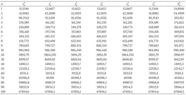
for 𝑚_]= 150, 𝑡_𝑘= 𝑘/], and ] = 5 by using Finite Difference method. In Table 1 an example of the computation of the eigenvalues of the operators𝐿(𝑞_𝑘) and 𝐿(𝑄_]) is given.

One can see fromTable 1that for𝑛 ≥ 30 the eigenvalues of the operators𝐿(𝑞_𝑘) and 𝐿(𝑄_V) are close to each other. This shows that the effect of the potential to the large eigenvalues is small. Moreover the eigenvalues in first, second, and third columns coincide with the eigenvalues in the sixth, fifth, and fourth columns, respectively, since the potential𝑞_𝑘(𝑥) can be reduced to𝑞_]−𝑘(𝑥) by using the transformation 𝑥 = 1 − 𝑧.

4. Comparison of the Asymptotic and

Numerical Methods

In this section we compare the estimations obtained by numerical and asymptotic methods of the eigenvaluesΛ2_𝑛of the operator𝐿(𝑄₂), where 𝑄₂is defined by (30) and (29). The 𝑛th eigenvalue of the operator 𝐿(0) is (𝑛𝜋)2_{. The effect of the}

potential𝑞_𝑘on the𝑛th eigenvalue 𝜆𝑘_𝑛 of the operator𝐿(𝑞_𝑘),

that is, the perturbation of the𝑛th eigenvalue when 𝐿(0) is perturbed by𝑞_𝑘is

𝑝𝑘_𝑛= 𝜆𝑘_𝑛− (𝑛𝜋)2. (33)

Similarly, the effect of𝑄₂on the𝑛th eigenvalue Λ2_𝑛, that is, the perturbation of the𝑛th eigenvalue when 𝐿(0) is perturbed by 𝑄₂is

𝑃_𝑛2= Λ2_𝑛− (𝑛𝜋)2. (34)

The perturbations 𝑃_𝑛2, 𝑝_𝑛𝑘 evaluated by the numerical and asymptotic methods are denoted by𝑃_𝑛2(𝑠), 𝑝𝑘_𝑛(𝑠), 𝑃_𝑛2(𝑎), and 𝑝𝑘

𝑛(𝑎), respectively.

According to Theorem 2 we define the approximate eigenvalues, denoted by𝑎_𝑛𝑘and𝐴2_𝑛, of the operators𝐿(𝑞_𝑘) and 𝐿(𝑄₂) obtained by the asymptotic method as follows

𝑎_𝑛𝑘= (𝑛𝜋)2+ ∫1 0 𝑞𝑘(𝑥) 𝑑𝑥 − ∫ 1 0 𝑞𝑘(𝑥) cos 2𝜋𝑛𝑥 𝑑𝑥, (35) 𝐴2_𝑛 = (𝑛𝜋)2+ ∫1 0 𝑄2(𝑥) 𝑑𝑥 − ∫ 1 0 𝑄2(𝑥) cos 2𝜋𝑛𝑥 𝑑𝑥. (36)

Therefore it is natural to define𝑃_𝑛2(𝑎) and 𝑝𝑘_𝑛(𝑎) by

𝑃_𝑛2(𝑎)=𝐴2_𝑛−(𝑛𝜋)2= ∫1 0 𝑄2(𝑥) 𝑑𝑥−∫ 1 0 𝑄2(𝑥) cos 2𝜋𝑛𝑥 𝑑𝑥, 𝑝𝑘_𝑛(𝑎) = 𝑎_𝑛𝑘− (𝑛𝜋)2= ∫1 0 𝑞𝑘(𝑥) 𝑑𝑥 − ∫ 1 0 𝑞𝑘(𝑥) cos 2𝜋𝑛𝑥 𝑑𝑥. (37) It readily follows from formulas (37) and (30) that

𝑃_𝑛2(𝑎) =∑2

𝑘=0

𝑝𝑘_𝑛(𝑎) . (38)

It means that for the large eigenvalues the effect of 𝑄₂ is asymptotically equal to the sum of the effects of the potentials 𝑞_𝑘.

The perturbations𝑃_𝑛2(𝑠) and 𝑝𝑘_𝑛(𝑠) evaluated via the finite difference method are given inTable 2. In order to see the effect of the singular points, the number of subintervals is taken as𝑚_]= 20000.

Table 2shows that the effect of𝑄₂is approximately within

the value range of5.10−5and2.10−2, equal to the sum of the effects of the potentials𝑞_𝑘. Thus the perturbation estimations by the numerical methods validate the naturality of (38).

(5)

Table 1 𝑛 𝑠0 𝑛 𝑠1𝑛 𝑠2𝑛 𝑠𝑛3 𝑠4𝑛 𝑠5𝑛 𝑆5𝑛 1 11,3346 12,0617 13,6112 13,6112 12,0617 11,3346 24,8946 2 41,0082 42,3680 42,5655 42,5655 42,3680 41,0082 54,4909 3 90,3543 92,1439 91,4556 91,4556 92,1439 90,3543 103,912 4 159,389 161,282 161,330 161,330 161,282 159,389 174,822 5 248,089 249,774 249,278 249,278 249,774 248,089 261,654 6 356,418 357,740 357,883 357,883 357,740 356,418 369,832 7 484,332 485,347 486,023 486,023 485,347 484,332 497,594 8 631,775 632,690 632,941 632,941 632,690 631,775 643,821 9 789,683 799,727 800,334 800,334 799,727 789,683 811,972 10 984,984 986,288 986,440 986,440 986,288 984,984 998,400 20 3892,79 3864,330 3894,39 3894,39 3864,330 3892,79 3906,97 30 8599,57 8600,85 8601,04 8601,04 8600,85 8599,57 8612,95 40 14902,3 14903,5 14903,7 14903,7 14903,5 14902,3 14915,3 50 22529,2 22530,6 22530,7 22530,7 22530,6 22529,2 22542,7 60 31151,4 31152,8 31152,8 31152,8 31152,8 31151,4 31165,1 70 40396,8 40398 40398,3 40398,3 40398 40396,8 40410,1 80 49866,8 49867,9 49868,2 49868,2 49867,9 49866,8 49879,9 90 59152,9 59154,3 59154,3 59154,3 59154,3 59152,9 59166,4 100 67854,6 67856,1 67856,1 67856,1 67856,1 67854,6 67868,3 Table 2 𝑛 𝑃2 𝑛(𝑠) 𝑝0𝑛(𝑠) 𝑝𝑛1(𝑠) 𝑝𝑛2(𝑠) ∑2𝑘=0𝑝𝑘𝑛(𝑠) |𝑝2𝑛(𝑠) − ∑2𝑘=0𝑝𝑘𝑛(𝑠)| 1 6,853010948 1,507680075 3,819522987 1,507680075 6,834883138 0,018127810 2 5,436436039 1,649044169 2,135885787 1,649044169 5,433974124 0,002461915 3 6,833127542 1,712792234 3,412323071 1,712792234 6,837907540 0,004779998 4 5,833596917 1,750983257 2,332560213 1,750983257 5,834526726 0,000929810 5 6,821354115 1,777106646 3,269640370 1,777106646 6,823853662 0,002499546 6 6,014222685 1,796412736 2,422163800 1,796412736 6,014989272 0,000766587 7 6,817074514 1,811422205 3,195628783 1,811422205 6,818473194 0,001398680 8 6,122590551 1,823514738 2,476005854 1,823514738 6,123035330 0,000444779 9 6,814993899 1,833516325 3,148677685 1,833516325 6,815710336 0,000716437 10 6,196675434 1,841954226 2,512821873 1,841954226 6,196730326 0,000054891 20 6,378247333 1,885045278 2,601825385 1,885045278 6,371915940 0,006331392

It is well known that if we consider the Sturm-Liouville operator

𝐿 (𝜀𝑄₂) = − 𝑑

𝑑𝑥2 + 𝜀𝑄2(𝑥) ,

𝑦 (0) = 𝑦 (1) = 0,

(39)

where 𝜀 is a small positive parameter, then the asymptotic methods can be applied more successfully. The𝑛th eigenvalue of the operators𝐿(𝜀𝑄_]) is denoted by Λ]_𝑛(𝜀). The approximate eigenvalues obtained by the asymptotic and numerical meth-ods are denoted by𝐴]_𝑛(𝜀) and 𝑆]_𝑛(𝜀), respectively.

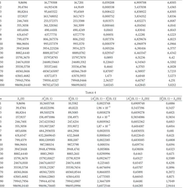
It follows fromTheorem 2and formulas (36), (30) that Λ2_𝑛(𝜀) = 𝐴2_𝑛(𝜀) + 𝑂 ((𝜀 ln |𝑛| 𝑛 ) 2 ) , (40) where 𝐴2_𝑛(𝜀) = (𝜋𝑛)2+ 𝜀 ∫1 0 𝑄2(𝑥) 𝑑𝑥 − 𝜀𝐶2𝑛 =(𝜋𝑛)2+𝜀 ∫1 0 ( 1 √|𝑥 − 1|+ 1 √|𝑥 − 1/2|+ 1 √|𝑥|) 𝑑𝑥 −𝜀 ∫1 0 ( 1 √|𝑥 − 1| + 1 √|𝑥 − 1/2| + 1 √|𝑥|) cos 2𝑛𝜋𝑥𝑑𝑥. (41) In Tables3,4, and5the approximate eigenvalues𝐴2_𝑛(𝜀) obtained by the asymptotic method and their comparison

(6)

Table 3 𝑛 𝜆_𝑛(0) 𝐴2 𝑛(1) 𝑆2𝑛(1) |𝐴2𝑛(1) − 𝑆2𝑛(1)| |𝐴2𝑛(1) − 𝜆𝑛(0)| |𝑆2𝑛(1) − 𝜆𝑛(0)| 1 9,8696 16,779308 16,7201 0,059208 6,909708 6,8505 2 39,4784 44,915438 44,9149 0,000538 5,437038 5,4365 3 88,8264 95,665322 95,6569 0,008422 6,838922 6,8305 4 157,9137 163,748052 163,7473 0,000752 5,834352 5,8336 5 246,7401 253,572371 253,5588 0,013571 6,832271 6,8187 6 355,3058 361,320361 361,3199 0,000461 6,014561 6,0141 7 483,6106 490,44101 490,4249 0,01611 6,83041 6,8143 8 631,6547 637,77751 637,7770 0,00051 6,12281 6,1223 9 799,4379 806,267576 806,2502 0,017376 6,829676 6,8123 10 986,9604 993,157379 993,1570 0,000379 6,196979 6,1966 20 3947,8418 3954,223216 3954,2175 0,005216 6,381416 6,3757 30 8882,6440 8889,107347 8889,0782 0,029347 6,463347 6,4342 40 15791,3670 15797,8793 15797,7870 0,0893 6,51236 6,42 50 24674,0110 24680,55663 24680,3312 0,22663 6,54563 6,3202 60 35530,5758 35537,1461 35536,6786 0,4661 6,5703 6,1028 70 48361,0616 48367,65097 48366,7849 0,87097 6,58937 5,7233 80 63165,4682 63172,073 63170,5955 1,473 6,6048 5,1273 90 79943,7956 79950,41327 79948,0466 2,36327 6,61767 4,251 100 98696,0440 98702,67245 98699,0652 3,60245 6,62845 3,0212 Table 4 𝑛 𝜆𝑛(0) 𝐴2𝑛(0, 1) 𝑆2𝑛(0, 1) |𝐴2𝑛(0, 1) − 𝑆2𝑛(0, 1)| |𝐴2𝑛(0, 1) − 𝜆𝑛(0)| |𝑆2𝑛(0, 1) − 𝜆𝑛(0)| 1 9,8696 10,5605748 10,5582 0,0023748 0,6909748 0,6886 2 39,4784 40,0221196 40,0221 1,96× 10−5 0,5437196 0,5437 3 88,8264 89,5103278 89,5085 0,0018278 0,6839278 0,6821 4 157,9137 158,4971086 158,4971 8,6× 10−6 0,5834086 0,5834 5 246,7401 247,4233362 247,4214 0,0019362 0,6832362 0,6813 6 355,3058 355,9072187 355,9072 1,87× 10−5 0,6014187 0,6014 7 483,6106 484,2936551 484,2916 0,0020551 0,6830551 0,681 8 631,6547 632,2669645 632,2668 0,0001645 0,6122645 0,6121 9 799,4379 800,1209185 800,1187 0,0022185 0,6830185 0,6808 10 986,9604 987,580134 987,5798 0,000334 0,619734 0,6194 20 3947,8418 3948,479906 3948,4741 0,005806 0,638106 0,6323 30 8882,6440 8883,2903 8883,2611 0,0291996 0,6463 0,6171 40 15791,3670 15792,01827 15791,9259 0,0923677 0,65127 0,5589 50 24674,0110 24674,66557 24674,4401 0,225465 0,65457 0,4291 60 35530,5758 35531,23287 35530,7654 0,4674694 0,65707 0,1896 70 48361,0616 48361,72051 48360,8544 0,8661055 0,65891 0,2072 80 63165,4682 63166,12865 63164,6511 1,4775505 0,66045 0,8171 90 79943,7956 79944,45741 79942,0907 2,3667109 0,66181 1,7049 100 98696,0440 98696,70685 98693,0996 3,6072546 0,66285 2,9444

with𝑆2_𝑛(𝜀) and nonperturbated eigenvalues 𝜆_𝑛(0) = (𝑛𝜋)2for 𝜀 = 1, 𝜀 = 0, 1, and 𝜀 = 0, 01, respectively, are given.

Table 3 shows the eigenvalues of 𝐿(𝜀𝑄₂) operator

obtained by asymptotic method and finite difference method, respectively, for𝜀 = 1. Here the number of subintervals is taken as𝑚_]= 15000.

obtained by asymptotic method and finite difference method, respectively, for 𝜀 = 0, 1. Here the number of subintervals is taken as𝑚_]= 15000.

obtained by asymptotic method and finite difference method, respectively, for 𝜀 = 0, 01. Here the number of subintervals is taken as𝑚_]= 15000.

5. Conclusion

It is natural and well known that for small values of the parameter𝜀 and for large eigenvalues the asymptotic method

(7)

Table 5 𝑛 𝜆_𝑛(0) 𝐴2 𝑛(0, 01) 𝑆2𝑛(0, 01) |𝐴2𝑛(0, 01) − 𝑆2𝑛(0, 01)| |𝐴2𝑛(0, 01) − 𝜆𝑛(0)| |𝑆2𝑛(0, 01) − 𝜆𝑛(0)| 1 9,8696 9,93870144 9,9385 0,00020144 0,06910144 0,0689 2 39,4784 39,53278781 39,5328 1,219× 10−5 0,05438781 0,0544 3 88,8264 88,89482843 88,8946 0,00022843 0,06842843 0,0682 4 157,9137 157,9720142 157,9720 1,423× 10−5 0,0583142 0,0583 5 246,7401 246,8084326 246,8082 0,00023264 0,0683326 0,0681 6 355,3058 355,3659045 355,3659 4,46× 10−6 0,0601045 0,0601 7 483,6106 483,6789196 483,6786 0,0003196 0,0683196 0,068 8 631,6547 631,71591 631,7158 0,00010995 0,06121 0,0611 9 799,4379 799,5062527 799,5058 0,00045269 0,0683527 0,0679 10 986,9604 987,0224095 987,0220 0,00040949 0,0620095 0,0616 20 3947,8418 3947,905575 3947,8998 0,00577499 0,063775 0,058 30 8882,6440 8882,708595 8882,6794 0,02919485 0,064595 0,0354 40 15791,3670 15791,43216 15791,3398 0,09236434 0,06516 0,0272 50 24674,0110 24674,07646 24673,8510 0,22545896 0,06546 0,16 60 35530,5758 35530,64155 35530,1740 0,46754647 0,06575 0,4018 70 48361,0616 48361,12746 48360,2614 0,86605935 0,06586 0,8002 80 63165,4682 63165,53422 63164,0567 1,47751533 0,06602 1,4115 90 79943,7956 79943,86183 79941,4951 2,36672503 0,06623 2,3005 100 98696,0440 98696,1103 98692,5031 3,60719526 0,0663 3,5409

gives us approximations with smaller errors. The numerical method, in general, gives better results for smaller eigenval-ues. The tables show that the results of the asymptotic method also give quiet acceptable results for small eigenvalues, since 𝐴2_𝑛(𝜀) − 𝑆2_𝑛(𝜀) is small.

Therefore we can easily observe that both of two methods give high-precision results for the calculation of the small eigenvalues. Additionally while the perturbation parameter tends to zero both of the methods are enhanced for smaller eigenvalues, but while this fact is limited to 𝑛 = 10 for the numerical approximation, the enhancement continues for the asymptotic method applied to higher eigenvalues. Thus we can conclude that the asymptotic method coupled with a perturbation parameter near to zero provides us a better approximation quality in calculating eigenvalues.

In Tables3–5there are two observations to be consid-ered: the first observation is that for small eigenvalues the perturbated results by numerical and asymptotic methods are close to each other for all𝜀. The second observation is that for the large eigenvalues the perturbated results obained by asymptotic methods decrease linearly with respect to small𝜀, while the perturbated results obtained by numerical methods are almost the same for all values of𝜀. This shows that for small values of the perturbation parameter𝜀 the asymptotic method is preferable.

Conflict of Interests

The authors of the paper do not have any direct or indirect financial relation with the commercial identities mentioned in the paper.

References

[1] B. Yilmaz and O. A. Veliev, “Asymptotic formulas for Dirichlet boundary value problems,” Studia Scientiarum

Mathemati-carum Hungarica, vol. 42, no. 2, pp. 153–171, 2005.

[2] O. A. Veliev and M. Toppamuk Duman, “The spectral expan-sion for a nonself-adjoint Hill operator with a locally integrable potential,” Journal of Mathematical Analysis and Applications, vol. 265, no. 1, pp. 76–90, 2002.

[3] G. D. Birkhoff, “Boundary value and expansion problems of ordinary linear differential equations,” Transactions of the

American Mathematical Society, vol. 9, no. 4, pp. 373–395, 1908.

[4] N. Dunford and J. T. Schwartz, Linear Operators. Part III, Spectral Operators, Wiley-Interscience, New York, NY, USA, 1988.

[5] W. N. Everitt, J. Gunson, and A. Zettl, “Some comments on Sturm-Liouville eigenvalue problems with interior singulari-ties,” Journal of Applied Mathematics and Physics, vol. 38, no. 6, pp. 813–838, 1987.

[6] V. A. Marchenko, Sturm-Liouville Operators and Applications, Birkh¨auser, Basel, Switzerland, 1986.

[7] M. A. Naimark, Linear Differential Operators, George G. Harrap and Company, 4th edition, 1967.

[8] B. N. Parlett, The Symmetric Eigenvalue Problem, Prentice-Hall, Englewood Cliffs, NJ, USA, 1980.

[9] J. D. Tamarkin, “Some general problems of the theory of ordi-nary linear differential equations and expansion of an arbitrary function in series of fundamental functions,” Mathematische

Zeitschrift, vol. 27, no. 1, pp. 1–54, 1928.

[10] E. C. Titchmarsh, Eigenfunction Expansions, vol. I, Oxford University Press, 1962.

[11] R. L. Burden, Numerical Analysis, Brooks Cole, Pacific Grove, Calif, USA, 7th edition, 2001.

(8)

[12] A. L. Andrew, “Correction of finite difference eigenvalues of periodic Sturm-Liouville problems,” Australian Mathematical

Society Journal Series B, vol. 30, no. 4, pp. 460–469, 1989.

[13] J. W. Paine, F. R. de Hoog, and R. S. Anderssen, “On the correction of finite difference eigenvalue approximations for Sturm-Liouville problems,” Computing, vol. 26, no. 2, pp. 123– 139, 1981.

[14] R. S. Anderssen and F. R. de Hoog, “On the correction of finite difference eigenvalue approximations for Sturm-Liouville problems with general boundary conditions,” BIT, vol. 24, no. 4, pp. 401–412, 1984.

[15] A. L. Andrew and J. W. Paine, “Correction of finite element estimates for Sturm-Liouville eigenvalues,” Numerische

Math-ematik, vol. 50, no. 2, pp. 205–215, 1986.

[16] C.-K. Chen and S.-H. Ho, “Application of differential trans-formation to eigenvalue problems,” Applied Mathematics and

Computation, vol. 79, no. 2-3, pp. 173–188, 1996.

[17] P. Ghelardoni, “Approximations of Sturm-Liouville eigenvalues using boundary value methods,” Applied Numerical

Mathemat-ics, vol. 23, no. 3, pp. 311–325, 1997.

[18] P. Ghelardoni and G. Gheri, “Improved shooting technique for numerical computations of eigenvalues in Sturm-Liouville problems,” Nonlinear Analysis, vol. 47, pp. 885–896, 2001. [19] J. D. Pryce, Numerical Solution of Sturm-Liouville Problems,

Clarendon Press, Oxford, UK, 1993.

[20] M. Kumar, “A new finite difference method for a class of singular two-point boundary value problems,” Applied Mathematics and

Computation, vol. 143, no. 2-3, pp. 551–557, 2003.

[21] M. Kumar and T. Aziz, “A uniform mesh finite difference method for a class of singular two-point boundary value problems,” Applied Mathematics and Computation, vol. 180, no. 1, pp. 173–177, 2006.

[22] M. Kumar and N. Singh, “A collection of computational techniques for solving singular boundary-value problems,”

Advances in Engineering Software, vol. 40, no. 4, pp. 288–297,

(9)

Submit your manuscripts at

http://www.hindawi.com

Hindawi Publishing Corporation

http://www.hindawi.com Volume 2014

Mathematics

Journal of

Mathematical Problems in Engineering

Hindawi Publishing Corporation http://www.hindawi.com

Differential Equations

International Journal of

Volume 2014

http://www.hindawi.com Volume 2014 Hindawi Publishing Corporationhttp://www.hindawi.com Volume 2014

Mathematical PhysicsAdvances in

Complex Analysis

Journal of

Optimization

Journal of

Combinatorics

International Journal of

Journal of Hindawi Publishing Corporation

Function Spaces

Abstract and Applied Analysis

http://www.hindawi.com Volume 2014 International Journal of Mathematics and Mathematical Sciences

Hindawi Publishing Corporation http://www.hindawi.com Volume 2014

The Scientific

World Journal

Discrete Dynamics in Nature and Society

Discrete Mathematics

Journal of

http://www.hindawi.com Volume 2014 Hindawi Publishing Corporationhttp://www.hindawi.com Volume 2014

Asymptotic and numerical methods in estimating eigenvalues

Research Article