C om mun.Fac.Sci.U niv.A nk.Series A 1 Volum e 66, N umb er 2, Pages 141–161 (2017) D O I: 10.1501/C om mua1_ 0000000808 ISSN 1303–5991
http://com munications.science.ankara.edu.tr/index.php?series= A 1
ROBUST PARAMETER ESTIMATION FOR THE MARSHALL-OLKIN EXTENDED BURR XII DISTRIBUTION
YE¸SIM GÜNEY AND OLCAY ARSLAN
Abstract. In this paper, we consider the parameter estimation of the Marshall– Olkin extended Burr XII (MOEBXII) distribution, which is a generalization of the Burr XII distribution. For the estimation of the parameters in the MOEBXII, maximum likelihood (ML) is available. However, this is not robust estimator. In this paper we proposed a robust estimator based on M estima-tion method to estimate the parameters of the MOEBXII distribuestima-tion. We perform a small simulation study to illustrate the performance of proposed method. We also reanalyze two data sets to asses the capability of the robust estimators over the ML and LS estimators.
1. Introduction
The Burr XII distribution [3] appears very often in practice when modelling unimodal data. Several researchers have investigated various inference problems using Burr distribution as it has been found useful in the study of actuarial science [11], economics [15], life testing and reliability, [1], [16], [17], failure time modeling [8] among others. The relationship between the Burr distribution and the various other distributions, is summarized by [18] and [21].
In the literature, various methods have been used to generalize Burr XII distri-bution. In addition Marshall and Olkin [14] introduced a method of adding a new parameter into a family of distributions. The resulting distribution is known as Marshall Olkin extended distribution. It is obtained as follows:
Let F (x) = 1 F (x) denote the survival function of a continuous random variable X. Then, the corresponding Marshall-Olkin (MO) extended distribution has survival function de…ned by
F (x) = F (x)
1 F (x) (1.1)
Received by the editors: December 10, 2016, Accepted: February 10, 2017.
2010 Mathematics Subject Classi…cation. Primary 05C38, 15A15; Secondary 05A15, 15A18. Key words and phrases. Marshall-Olkin extended Burr XII (MOEBXII) distribution, robust estimator,maximum likelihood estimator, least squares estimator.
c 2 0 1 7 A n ka ra U n ive rsity C o m m u n ic a tio n s d e la Fa c u lté d e s S c ie n c e s d e l’U n ive rs ité d ’A n ka ra . S é rie s A 1 . M a th e m a t ic s a n d S t a tis t ic s .
where > 0 and = 1 . The new family contains the initial family as a particular case, obtained when = 1.
There have been various studies reported in the literature dealing with the para-meter estimation methods for Burr XII distribution. ML estimation of parapara-meters for …tting Burr distribution to life test data has been studied by [22] and [23]. ML and maximum product of spacings (MPS) methods were compared by [19]. In addition, estimation of parameters in the presence of outliers for a Burr XII dis-tribution with LS, ML and MPS methods were compared by [9]. The minimum variance linear unbiased estimators (MVLUE), the best linear invariant estimators (BLIE) and the maximum likelihood estimators (MLE) based on n-selected gener-alized order statistics are presented for the parameters of the Burr XII distribution by [13]. An alternative robust estimation methods based on M estimators and op-timal B-robust estimation method for the parameters of Burr XII distribution have been proposed by [4] and [5], respectively. However, there is not much work for MOEBXII distribution. The parameters of MOEBXII distribution was estimated by using ML estimation method by [2]. However, it is well established that in the presence of outliers in the data, the traditional methods do not provide reliable estimations. Therefore robust estimation methods can be used for the parameters of the MOEBXII distribution if the data contains outliers.
In this paper, we propose a robust estimation procedures based on M-estimation method to estimate the parameters of the MOEBXII distribution. This is done by changing LS objective function with robust objective function and minimizing it. We compare the performance of the method with the ML and LS estimation methods by a simulation study and real data examples.
The rest of the paper is organized as follows; In section 2, we described the MOEBXII distribution. The maximum likelihood estimator and least square esti-mator are provided in sections 3. In section 4, simulation results are presented. In Section 5, we reanalyze two data sets for illustrative purpose. Finally, conclusions are given in section 6.
2. Marshall-Olkin Extended Burr XII Distribution
A random variable X is said to have a Burr XII distribution with shape para-meters c > 0 and k > 0 if its probability density function (pdf) is given by
f (x; c; k) = ck x
(c 1)
(1 + xc)k+1; x 0: (2.1)
The cumulative density function (cdf) of X is given by
F (x; c; k) = 1 1
Substituting (2.2) in (1.1) we obtain a Marshall-Olkin Extended Burr XII distrib-ution denoted by M OEBXII( ; c; k) with the following pdf and cdf
f (x; ; c; k) = ck x (c 1)(1 + xc) (k+1) [1 (1 ) (1 + xc) k]2; x 0: (2.3) F (x; ; c; k) = 1 (1 + x c) k 1 (1 ) (1 + xc) k; x 0: (2.4)
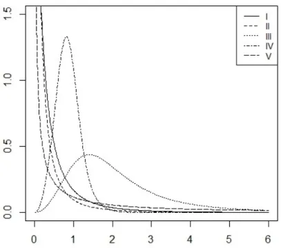
where ,c and k > 0 [2]. Note that the MOEBXII distribution is an extended model to analyze more complex data and it generalizes some of the distributions. In particular for = 1 MOEBXII becomes Burr XII distribution with two parameters c and k. And also, when c = 1, the MOEBXII becomes the Marshall-Olkin extended Lomax distribution. Clearly, MOEBXII distribution is more ‡exible than the Burr XII distribution, because of the presence of the shape parameter. Figure 1 shows the plots of pdf for MOEBXII distribution for some values of the parameters. For more details, see [2].
Figure 1. Plot of pdf of the MOEBXII distribution. (I) = 1; c = 0:9; k = 3; (II) = 0:5; c = 0:9; k = 3; (III) = 5; c = 3; k = 0:9; (IV) = 3; c = 3; k = 3; (V) = 0:8; c = 0:7; k = 0:8
3. Estimation of the Parameters of MOEBXII Distribution In this study to estimate ; c and k, we consider ML, LS and robust estimation methods.
3.1. Maximum Likelihood Estimation of MOEBXII Distribution. Let x = (x1; x2; :::; xn) be a random sample from M OEBXII( ; c; k). In order to estimate
the parameters of the MOEBXII distribution, the log-likelihood of the sample is maximized with respect to the parameters. Log-likelihood function can be written as l( ; c; k) = n log ( ck) + (c 1) n X i=1 log xi (k + 1) n X i=1 log (1 + xci) 2 n X i=1 log 1 (1 ) (1 + xci) k (3.1)
The associated nonlinear loglikelihood system for MLE’s is @l @ = n 2 n X i=1 (1 + xc i) k 1 (1 ) (1 + xc i) k = 0 (3.2) @l @c = n c + n X i=1 log xi (k + 1) n X i=1 xcilog (xi) (1 + xc i) 2k(1 ) n X i=1 xci(1 + xci) (k+1)log (xi) 1 (1 ) (1 + xc i) k = 0 (3.3) @l @k = n k n X i=1 log (1 + xci) (k + 1) n X i=1 xc ilog (xi) (1 + xc i) 2(1 ) n X i=1 (1 + xci) klog(1 + xci) 1 (1 ) (1 + xc i) k = 0: (3.4)
Notice that there are no explicit solutions to (3.2),(3.3) and (3.4). Hence, numerical methods are applied to solve the required equations.
3.2. Least Squares Estimation Method of MOEBXII Distribution. In this section we will discuss the least squares method for estimating ; c and k. As for the Burr XII distribution [4], LS estimation method can be used as an alternative to the ML estimation method to estimate the parameters of the MOEBXII distribution.
The LS method is a combination of parametric (F ) and non-parametric Fb distribution functions. The procedure attempts to minimize the following function
with respect to ; c and k S( ; c; k) = n X i=1 b F (xi) F (xi) 2 (3.5) = n X i=1 b F (xi) 1 (1 + xci) k 1 (1 ) (1 + xc i) k 2 : (3.6)
Since the cdf of MOEBXII does not have a linear form according to the para-meters, it will be di¢ cult to minimize the equation (3.6). For this reason, we get the linear form of F (x) : To obtain the linear form of F (x) ; we use the following transformation
log log 1
1 F (x) = log log ( 1) log log ( ) + log (k) + log log(1 + x
c i):
Instead of minimizing the squares of the di¤erence between the bF ( ) and F ( ), we minimize the squares of the di¤erence between the linear form of F ( ) and the same transformation of bF ( ).
On the other hand, bF (x) is unknown, we use bFX(i)(x) as follows
b
FX(i)(x) =
i 0:5
n ; i = 1; 2; :::; n (3.7)
where X(i) is the i: order statistics of the random sample of the size n from
MOE-BXII distribution. Hence for the MOEMOE-BXII distribution, to obtain thee LS esti-mates bLS;bcLS;and bkLS of the parameters ; c and k we can de…ne the following
objective function:
S( ; c; k) =
n
X
i=1
y(i) log log ( 1) + log log ( ) log (k) log log(1 + xc(i)) 2
(3.8) where y(i)= log log 1 Fb1
X(i)(x) : The goal is to …nd ; c and k that minimize the
objective function. This requires us to …nd the values of ; c and k such that
n
X
i=1
y(i) log log ( 1) + log log ( ) log (k) log log(1 + xc(i)) = 0; (3.9)
n
X
i=1
0
@ y(i) log log ( 1) + log log ( ) log (k) log log(1 + x
c (i)) xc(i)log(x(i))
(1+xc (i)) log(1+x c (i)) 1 A = 0; (3.10) y log log ( 1) + log log ( ) log k 1
n
n
X
i=1
3.3. Robust Estimation for the MOEBXII Distribution. We observe that, as in the Burr XII distribution case, the score functions for c and k are unbounded function of x. This implies that the ML estimators for c and k may be a¤ected from outliers in data. It is also happens for the LS estimators as well since the objective function for the LS method and the corresponding score functions are unbounded function of x. This can be easily checked from the equation (3.3)-(3.4) and (3.10)-(3.11). Therefore in the presence of outliers, instead of using ML or LS estimation methods robust methods should be used to get estimators that are not sensitive to the outliers.
In this paper we proposed a robust estimation method based on M estimation method proposed by Huber [10]. In this method we will use a objective function, say as in used in robustness theory which is less decreasing than square function or bounded to reduced the e¤ect of outliers on the estimators. The method will be carried out as follows. We will be minimize following objective function with respect to the parameters of interest instead of minimizing of the objective function given in equation (3.8) or maximizing the loglikelihood function given in equation (3.1).
Q( ; c; k) =
n
X
i=1
(yi log log ( 1) + log log ( ) log (k) log log(1 + xci)) :
(3.12) By taking the derivatives of the objective function Q with respect to the parameters we obtain following equations
@Q( ; c; k)
@ =
n
X
i=1
0(yi log log ( 1) + log log ( ) log (k) log log(1 + xc i)) 1 1 log( 1) 1 log( ) ! = 0; (3.13) @Q( ; c; k) @c = n X i=1
0(yi log log ( 1) + log log ( ) log (k) log log(1 + xc i)) xc ilog(xi) (1+xc i) log(1+xci) ! = 0; (3.14) @Q( ; c; k) @k = n X i=1 0(y
i log log ( 1) + log log ( ) log (k) log log(1 + xci))
k = 0:
(3.15) There many functions used in robust statistical analysis. However, since Huber’s and Tukey’s functions are widely used in literature we will use Huber’s and Tukey’s
functions. This functions are
(x) = x
2 ;
jxj b1
(x) = ( 1 1 (x=b2)2 2 ; jxj b2 1 ; jxj > b2 ; (3.17)
respectively. Here b1 and b2 are called the robustness tuning constants After
re-arranging the equations (3.13), (3.14) and (3.15) these estimates can also be ob-tained by solving the nonlinear equations:
log bk = n X i=1 !iyi n X i=1 !i n X i=1 !ilog log(1 + xci) n X i=1 !i
log log ( 1) + log log ( ) ; (3.18)
n
X
i=1
!i(yi log log ( 1) + log log ( ) log (k) log log(1 + xci)) xcilog(xi) (1+xc i) log(1+xci) ! = 0; (3.19)
log (log ( ) log ( 1)) =
n X i=1 !iyi n X i=1 !i n X i=1 !ilog log(1 + xci) n X i=1 !i log(k) (3.20)
where !i’s are the weights. When the Huber’s function is used, the weights will
be
!i= min 1;
b1
j(yi log log ( 1) + log log ( ) log (k) log log(1 + xci))j
: (3.21) If the Tukey’s function is used, the weights will be
!i=
0
@ 1 (yi log log( 1)+log log( ) log(k) log log(1+x
c i))
b2
2 2
I(j(yi log log ( 1) + log log ( ) log (k) log log(1 + xci))j b2)
1 A : (3.22) 4. Simulation Study
Generating data from the MOEBXII distribution. For the Burr distribu-tion the data generating procedures are available in literature (e.g., random(’burr’,c,k) code in Matlab). However for the MOEBXII distribution, we can not be able to see any available data generating procedures. Therefore, before the simulation study we will give a brief outline of the data generating scheme use in our simulation study for the MOEBXII distribution.
We generate the data from the MOEBXII distribution by using Inverse Trans-form Method. First we generate random numbers u1; u2; :::; un from the uniform
distribution on the interval (0; 1). Then we …nd the inverse of cdf of the MOEBXII distribution F 1( ) for any given ; c and k values and calculate the value F 1(u
i)
for i = 1; 2; :::; n:
Next, we provide a small simulation study to compare the performance of the estimation methods given in section 3. We generate N=100 samples of size n (n = 20, n = 40, and n = 100) from the MOEBXII distribution. We have taken parameter values ( ; c; k) = (3; 1; 1); (3; 1; 2); (3; 2; 1); (3; 2; 2); (3; 3; 3); (5; 1; 1); (5; 1; 2); (5; 2; 1) and (5; 2; 2).
To assess the performance of the methods, we calculated the bias and the RMSE for the estimates of = ; c and k obtained from the simulated data sets
Bias b = 1 N n X i=1 bi ; (4.1) RM SE = b = v u u t 1 N n X i=1 bi 2: (4.2)
Robust estimations of the parameters are obtained with tuning constant b1= 3:5
for Huber’s function and b2= 1:345 for Tukey’s function.
The results of our simulation study are presented in the Tables 1–6. In the tables, we present the bias and RMSE for the estimators obtain from the methods described in Section 3.
The results of our simulation study for the data sets without outliers are pre-sented in the Tables 1–3. This results show that all estimation methods considered in this paper perform well in estimating the parameters of the MOEBXII distribu-tion when the data sets do not contain any outliers. However the robust estimator based on Tukey’s function generally outperforms others in terms of the bias and RMSE. In addition, the average bias and RMSE of all the estimators of the para-meters c and k generally decrease as n increases.
Table 1 The Bias and RMSE (Parenthesis) for n = 20 Parameter ML LS Huber Tukey (3; 1; 1) 0.2703 (0.2907) 0.3599 (0.4274) 0.3411 (0.4149) 0.2356 (0.3806) (3; 1; 2) 0.1239 (0.1820) 0.1928 (0.5397) 0.1267 (0.2185) 0.0078 (0.1872) (3; 2; 1) 0.5183 (0.5499) 0.2208 (0.6144) 0.5446 (0.5664) 0.5362 (0.5612) (3; 2; 2) 0.1034 (0.2470) 0.2287 (0.2971) 0.0957 (0.2843) 0.0892 (0.2538) (3; 3; 3) 0.3755 (1.1090) 0.1285 (0.3726) 0.1462 (0.1916) 0.0967 (0.1970) (5; 1; 1) 0.0965 (0.3055) 0.3622 (0.3786) 0.0727 (0.2655) 0.0437 (0.2282) (5; 1; 2) 0.3204 (0.6993) 0.1776 (0.1887) 0.1955 (0.1976) 0.1962 (0.1981) (5; 2; 1) 0.4591 (0.6376) 0.2003 (0.4086) 0.2413 (0.4166) 0.2160 (0.4063) (5; 2; 2) 0.1620 (0.1857) 0.4056 (0.8534) 0.1660 (0.1854) 0.1358 (0.2245)
Parameter c. ML LS Huber Tukey (3; 1; 1) 0.5789 (0.5822) 0.5851 (0.5870) 0.5824 (0.5857) 0.2436 (0.3245) (3; 1; 2) 0.5885 (0.5924) 0.8937 (0.9443) 0.5913 (0.5934) 0.5821 (0.5891) (3; 2; 1) 0.1333 (0.3235) 0.0531 (0.3903) 0.1097 (0.3149) 0.1511 (0.3153) (3; 2; 2) 0.2093 (0.3370) 0.2346 (0.3390) 0.2071 (0.3297) 0.0310 (0.4851) (3; 3; 3) 0.1599 (0.1974) 0.1651 (0.3172) 0.1559 (0.1954) 0.1506 (0.1953) (5; 1; 1) 0.6275 (0.6698) 0.5779 (0.5891) 0.5948 (0.5958) 0.5833 (0.5909) (5; 1; 2) 0.6766 (0.7201) 0.5990 (0.5990) 0.5975 (0.5976) 0.5924 (0.5945) (5; 2; 1) 0.3222 (0.4300) 0.1843 (0.3417) 0.2328 (0.3456) 0.2003 (0.4086) (5; 2; 2) 0.3137 (0.4210) 0.2769 (0.3694) 0.2755 (0.3883) 0.2744 (0.3837) Parameter k. ML LS Huber Tukey (3; 1; 1) 0.5785 (0.5801) 0.4808 (0.5291) 0.5768 (0.5780) 0.3869 (0.4556) (3; 1; 2) 0.1279 (0.1502) 0.3546 (0.5322) 0.1682 (0.1813) 0.0695 (0.1335) (3; 2; 1) 0.5843 (0.5863) 0.5950 (0.5951) 0.5937 (0.5941) 0.3517 (0.4567) (3; 2; 2) 0.1526 (0.3134) 0.3803 (1.0688) 0.1392 (0.3096) 0.1222 (0.2978) (3; 3; 3) 0.5488 (0.8331) 0.1878 (0.3971) 0.1105 (0.2105) 0.0388 (0.2250) (5; 1; 1) 0.3524 (0.3930) 0.4922 (1.0249) 0.3981 (0.4235) 0.1626 (0.3129) (5; 1; 2) 0.2053 (0.5287) 0.1955 (0.1986) 0.1933 (0.1998) 0.1908 (0.1949) (5; 2; 1) 0.4993 (0.5164) 0.1628 (0.2043) 0.5051 (0.5200) 0.4935 (0.5164) (5; 2; 2) 0.5043 (0.6367) 0.2200 (0.5748) 0.1571 (0.2087) 0.1406 (0.2272)
Table 2 The Bias and RMSE (Parenthesis) for n = 40 Parameter ML LS Huber Tukey (3; 1; 1) 0.3787 (0.4215) 0.4084 (0.4373) 0.3134 (0.4223) 0.0038 (0.3636) (3; 1; 2) 0.1859 (0.2659) 0.1996 (0.2629) 0.1547 (0.4467) 0.0543 (0.7690) (3; 2; 1) 0.4862 (0.4918) 0.2783 (0.2840) 0.4365 (0.6060) 0.3921 (0.5403) (3; 2; 2) 0.1259 (0.3692) 0.0921 (0.2560) 0.7029 (0.5622) 0.0751 (0.2333) (3; 3; 3) 0.1303 (1.3301) 0.2127 (0.3781) 0.2281 (0.4004) 0.0077 (0.2743) (5; 1; 1) 0.4041 (0.5928) 0.2336 (0.4158) 0.3505 (0.3610) 0.2873 (0.4083) (5; 1; 2) 0.2633 (0.5182) 0.3413 (0.3626) 0.2618 (0.4991) 0.4320 (0.4531) (5; 2; 1) 0.4017 (0.4121) 0.1647 (0.4358) 0.4194 (0.4307) 0.2258 (0.4345) (5; 2; 2) 0.2049 (0.3830) 0.1414 (0.3478) 0.4065 (0.8821) 0.0230 (0.2731) Parameter c. ML LS Huber Tukey (3; 1; 1) 0.2311 (0.3102) 0.4149 (0.5571) 0.4917 (0.4938) 0.4959 (0.4963) (3; 1; 2) 0.2269 (0.2810) 0.4959 (0.4966) 0.3990 (0.3361) 0.2941 (0.4973) (3; 2; 1) 0.0258 (0.3802) 0.0706 (0.3337) 0.0706 (0.3244) 0.0201 (0.2980) (3; 2; 2) 0.1390 (0.3383) 0.1886 (0.3392) 0.0661 (0.448 ) 0.0259 (0.4815) (3; 3; 3) 1.0137 (1.0836) 0.4633 (0.4712) 0.9990 (1.0880) 0.4329 (0.4646) (5; 1; 1) 0.6905 (0.7355) 0.4969 (0.4973) 0.6500 (0.6931) 0.4017 (0.4121) (5; 1; 2) 0.7259 (0.7683) 0.4041 (0.5928) 0.6964 (0.7622) 0.1573 (0.3372) (5; 2; 1) 0.3261 (0.4219) 0.1493 (0.3335) 0.3581 (0.4144) 0.0964 (0.3111) (5; 2; 2) 0.3466 (0.4326) 0.3076 (0.4397) 0.2061 (0.3551) 0.1573 (0.3372) Parameter k. ML LS Huber Tukey (3; 1; 1) 0.3658 (0.5287) 0.4905 (0.4908) 0.4883 (0.4891) 0.0275 (0.2457) (3; 1; 2) 0.3934 (0.4905) 0.0275 (0.2457) 0.3731 (0.5183) 0.0037 (0.2295) (3; 2; 1) 0.4956 (0.4970) 0.4894 (0.4913) 0.4981 (0.4983) 0.2336 (0.4158) (3; 2; 2) 0.3340 (0.7965) 0.1092 (0.2957) 0.4097 (0.9214) 0.1069 (0.2704) (3; 3; 3) 0.6937 (0.9322) 0.2630 (0.3787) 0.7339 (0.9491) 0.2061 (0.3796) (5; 1; 1) 0.3255 (0.3471) 0.3274 (0.3567) 0.3466 (0.4326) 0.1647 (0.4358) (5; 1; 2) 0.6905 (0.7355) 0.4834 (0.4858) 0.4969 (0.4973) 0.2463 (0.7562) (5; 2; 1) 0.6937 (0.9322) 0.4312 (0.4451) 0.4480 (0.4588) 0.2630 (0.3787) (5; 2; 2) 0.8649 (1.0009) 0.3702 (0.4095) 0.3261 (0.4219) 0.1069 (0.2704)
Table 3 The Bias and RMSE (Parenthesis) for n = 100 Parameter ML LS Huber Tukey (3; 1; 1) 0.0597 (0.1429) 0.0835 (0.1021) 0.0721 (0.1037) 0.0115 (0.1037) (3; 1; 2) 0.1491 (0.2890) 0.2981 (0.3841) 0.0785 (0.3016) 0.0332 (0.1245) (3; 2; 1) 0.0180 (0.1225) 0.1465 (0.5922) 0.1798 (0.1927) 0.1968 (0.1981) (3; 2; 2) 0.0517 (0.2840) 0.0887 (0.2847) 0.0376 (0.1207) 0.0257 (0.3115) (3; 3; 3) 0.0926 (0.4129) 0.1635 (0.3879) 0.0513 (0.1556) 0.0056 (0.4082) (5; 1; 1) 0.0222 (0.1335) 0.0316 (0.1361) 0.0941 (0.1611) 0.0142 (0.1323) (5; 1; 2) 0.0459 (0.1172) 0.0364 (0.1514) 0.0507 (0.1162) 0.0178 (0.1341) (5; 2; 1) 0.1982 (0.1983) 0.1615 (0.4114) 0.2118 (0.3724) 0.2113 (0.3707) (5; 2; 2) 0.1486 (0.3654) 0.2067 (0.3864) 0.1867 (0.3723) 0.0929 (0.1024) Parameter c ML LS Huber Tukey (3; 1; 1) 0.0385 (0.1419) 0.0842 (0.5175) 0.1946 (0.1970) 0.0094 (0.1324) (3; 1; 2) 0.4973 (0.4977) 0.4986 (0.4988) 0.4974 (0.4978) 0.1995 (0.1996) (3; 2; 1) 0.1797 (0.3181) 0.1242 (0.2960) 0.0992 (0.2954) 0.0005 (0.3589) (3; 2; 2) 0.1962 (0.3680) 0.2169 (0.3439) 0.1979 (0.3686) 0.0262 (0.1352) (3; 3; 3) 0.3345 (0.4441) 0.3354 (0.4510) 0.3430 (0.4567) 0.0949 (0.1011) (5; 1; 1) 0.0932 (0.1025) 0.0957 (0.1010) 0.0978 (0.1625) 0.0143 (0.1275) (5; 1; 2) 0.1264 (0.1750) 0.1594 (0.1857) 0.1570 (0.1861) 0.1075 (0.0459) (5; 2; 1) 0.2646 (0.3608) 0.1864 (0.3436) 0.2230 (0.3498) 0.1197 (0.3876) (5; 2; 2) 0.1363 (0.3576) 0.1601 (0.3279) 0.1597 (0.3565) 0.0270 (0.1173) Parameter k ML LS Huber Tukey (3; 1; 1) 0.0864 (0.1024) 0.0831 (0.1013) 0.0913 (0.1539) 0.0562 (0.0975) (3; 1; 2) 0.1844 (0.3232) 0.1977 (0.1982) 0.1170 (0.3341) 0.0257 (0.2820) (3; 2; 1) 0.0501 (0.1433) 0.2524 (0.7771) 0.0529 (0.1413) 0.0509 (0.1416) (3; 2; 2) 0.0859 (0.3318) 0.1380 (0.1779) 0.0259 (0.3263) 0.0814 (0.3295) (3; 3; 3) 0.1643 (0.3750) 0.2457 (0.3703) 0.1148 (0.3868) 0.0753 (0.1087) (5; 1; 1) 0.1767 (0.1866) 0.1791 (0.1873) 0.1597 (0.1814) 0.1088 (0.0423) (5; 1; 2) 0.3285 (0.4698) 0.1405 (0.1637) 0.1767 (0.1866) 0.1597 (0.1814) (5; 2; 1) 0.4746 (0.9614) 0.4583 (0.4710) 0.3553 (0.4097) 0.1172 (0.1600) (5; 2; 2) 0.3160 (0.4152) 0.3311 (0.4163) 0.3117 (0.4193) 0.1878 (0.1942)
Table 4–6 list the bias and RMSE for the data sets with outliers. For the sample size n = 20, there is one outlier, for the sample sizes n = 40 and n = 100, there are two and four outliers, respectively. The outliers are taken 100 largest observation. From Tables 4-6, we observe that outliers induce a large in‡uence on the bias and RMSE of the ML and LS estimators. In particular the ML and LS estimators
compared to the robust estimators are drastically e¤ected from the outliers when the number of outliers is four.
The simulation results in Tables 4-6 clearly indicates that the robust estimator based on Tukey’s function has the smallest bias in all cases and smallest RMSE in most of the cases with outliers. In addition, the robust estimator based on Huber’s function outperforms LS and ML estimator in terms of bias and RMSE when the data set contains outlier. For example it can be seen from Tables 4-6 that the largest di¤erence of bias for parameter c arises in Table 4 for the cases (3,2,2) and (5,2,2) and for the parameter k the same happens for the cases (5,1,2) and (5,2,1). Similarly we can observe superiority of the robust estimators in terms of bias and RMSE in Tables 5-6.
Finally in Table 6 we observe that when the number of outliers increases, the LS and the ML estimators dramatically worsen compared to the robust estimators. It can be seen that bias and the RMSE values are very large for the LS and ML estimators.
Table 4 The Bias and RMSE (Parenthesis) for n = 20 with one outlier Parameter ML LS Huber Tukey (3; 1; 1) -0.8720 (0.8857) 0.1889 (0.1939) -0.0467 (0.4116) 0.0399 (0.1566) (3; 1; 2) -0.8637 (0.9271) -0.8936 (0.9683) -0.1737 (0.1887) 0.0103 (0.4528) (3; 2; 1) -0.8621 (0.9096) 0.1848 (0.1911) 0.1845 (0.2419) 0.1663 (0.1856) (3; 2; 2) -0.7024 (1.7847) -0.7262 (0.7852) -0.0939 (0.1828) 0.0376 (0.2696) (3; 3; 3) 0.4533 (0.9336) -0.3358 (0.6387) -0.1379 (0.1944) -0.1262 (0.1953) (5; 1; 1) -0.9716 (0.9736) -0.5881 (0.7478) -0.0861 (0.1790) 0.0148 (0.1702) (5; 1; 2) 0.8130 (0.8402) -0.7250 (0.7646) 0.0324 (0.5353) -0.0025 (0.1813) (5; 2; 1) 0.9896 (1.0093) -0.1615 (0.3716) 0.1293 (0.1579) 0.0768 (0.1479) (5; 2; 2) -0.9334 (0.9401) -0.4343 (0.7769) -0.1725 (0.1992) 0.0688 (0.5022) Parameter c ML LS Huber Tukey (3; 1; 1) 0.4250 (0.5100) 0.8450 (0.8713) 0.1939 (0.1961) 0.1930 (0.1963) (3; 1; 2) 0.4187 (0.5125) 0.8329 (0.8595) 0.1986 (0.1988) 0.1976 (0.1981) (3; 2; 1) -0.6027 (0.6895) 0.1951 (0.1966) -0.0545 (0.0575) 0.0190 (0.0200) (3; 2; 2) -0.6474 (0.7040) -1.2856 (1.7346) 0.0821 (0.2429) -0.0689 (0.0713) (3; 3; 3) -0.9999 (0.9999) -0.7101 (0.8230) -0.1903 (0.1966) -0.0928 (0.1877) (5; 1; 1) 0.6388 (0.6456) 0.8683 (0.8889) 0.0414 (0.2640) -0.0080 (0.0714) (5; 1; 2) 0.5336 (0.6383) -0.6467 (0.7541) 0.1995 (0.1996) 0.1617 (0.1958) (5; 2; 1) -0.8357 (0.8441) 0.2568 (0.2670) 0.1131 (0.5104) 0.0395 (0.4005) (5; 2; 2) 1.6584 (1.6625) -0.5162 (0.5476) -0.4642 (0.4703) -0.1641 (0.2074)
Parameter k ML LS Huber Tukey (3; 1; 1) 0.4511 (0.5099) 0.7417 (0.7680) 0.1979 (0.1981) 0.0301 (0.1697) (3; 1; 2) -0.5508 (0.6172) 0.2754 (0.2825) -0.4002 (0.4035) -0.1672 (0.5026) (3; 2; 1) 0.4795 (0.5475) 0.5920 (0.6455) 0.1653 (0.1911) -0.0312 (0.4778) (3; 2; 2) -0.3657 (0.4728) -0.3149 (0.4629) 0.1476 (0.2398) -0.0444 (0.0898) (3; 3; 3) -0.9983 (0.9983) -0.1501 (0.6614) -0.1480 (0.1900) -0.1294 (0.1969) (5; 1; 1) 0.4275 (0.4415) 0.8678 (0.8734) 0.3440 (0.4601) 0.0070 (0.0097) (5; 1; 2) 1.1828 (1.3903) 0.2941 (0.3833) 0.1354 (0.1590) -0.0880 (0.1827) (5; 2; 1) -0.7448 (0.7760) 1.1564 (1.1823) -0.5800 (0.5275) 0.0758 (0.4103) (5; 2; 2) -0.8840 (0.9824) 0.3214 (0.4134) 0.1406 (0.1705) 0.1053 (0.1702) Table 5 The Bias and RMSE (Parenthesis) for n = 40 with two outliers Parameter ML LS Huber Tukey (3; 1; 1) -0.8720 (0.8857) 0.8450 (0.8713) 0.1889 (0.1939) 0.0399 (0.1566) (3; 1; 2) -0.8637 (0.9271) -0.7101 (0.8230) -0.1936 (0.1968) -0.1737 (0.1887) (3; 2; 1) -0.8621 (0.9096) 0.2845 (0.4419) 0.1848 (0.1911) 0.1663 (0.1856) (3; 2; 2) 1.1558 (1.3132) 0.8130 (0.8402) -0.0939 (0.1828) -0.1617 (0.1938) (3; 3; 3) 0.4533 (0.9336) -0.3358 (0.6387) -0.1379 (0.1944) -0.1262 (0.1953) (5; 1; 1) 1.2561 (1.2758) 1.1057 (1.1161) 0.0688 (0.5022) -0.0861 (0.1790) (5; 1; 2) -0.9467 (0.9541) 1.2686 (1.2866) 0.1995 (0.1996) 0.1617 (0.1958) (5; 2; 1) -1.4959 (1.4992) 1.2676 (1.2897) 0.1293 (0.1579) 0.0768 (0.1479) (5; 2; 2) 1.1825 (1.2136) -2.7170 (2.7186) 0.0539 (0.1066) 0.1976 (0.3438) Parameter c ML LS Huber Tukey (3; 1; 1) 0.4250 (0.5100) 0.7417 (0.7680) 0.1939 (0.1961) 0.1930 (0.1963) (3; 1; 2) 0.4187 (0.5125) 0.8683 (0.8889) 0.1986 (0.1988) 0.1976 (0.1981) (3; 2; 1) -0.6027 (0.6895) 0.5920 (0.6455) 0.0376 (0.2696) 0.0324 (0.5353) (3; 2; 2) -0.6474 (0.7040) -0.7250 (0.7646) 0.0450 (0.4822) 0.0148 (0.1702) (3; 3; 3) -0.9999 (0.9999) -0.7448 (0.7760) -0.0928 (0.1877) -0.1903 (0.1966) (5; 1; 1) -0.5716 (0.5736) 0.5824 (0.6063) 0.1999 (0.1999) 0.0395 (0.4005) (5; 1; 2) -0.4312 (0.4346) -0.4775 (0.4997) -0.1725 (0.1992) -0.0025 (0.1813) (5; 2; 1) -0.8357 (0.8441) 0.8007 (0.8093) -0.1306 (0.6490) 0.0218 (0.0226) (5; 2; 2) -0.9334 (0.9401) 0.2990 (0.3033) 0.1131 (0.5104) 0.0326 (0.1214)
Parameter k ML LS Huber Tukey (3; 1; 1) 0.4511 (0.5099) 0.8329 (0.8595) 0.1979 (0.1981) 0.0301 (0.1697) (3; 1; 2) -0.5508 (0.6172) -0.1672 (0.5026) -0.0312 (0.4778) 0.0103 (0.4528) (3; 2; 1) 0.4795 (0.5475) -0.5881 (0.7478) 0.1951 (0.1966) 0.1653 (0.1911) (3; 2; 2) -0.3657 (0.4728) -0.3149 (0.4629) 0.2941 (0.3833) -0.1501 (0.6614) (3; 3; 3) -0.9983 (0.9983) 0.8211 (0.8301) -0.1480 (0.1900) -0.1294 (0.1969) (5; 1; 1) 0.9388 (0.9456) -0.7595 (0.7975) 0.1354 (0.1590) -0.0880 (0.1827) (5; 1; 2) 0.9336 (0.9383) 0.3214 (0.4134) 0.1406 (0.1705) 0.1053 (0.1702) (5; 2; 1) 0.2870 (0.3752) -0.3589 (0.3638) -0.1189 (0.6799) -0.0262 (0.1368) (5; 2; 2) 0.3440 (0.4601) 0.7412 (0.7497) -0.0560 (0.0581) 0.0363 (0.0383)
Table 6 The Bias and RMSE (Parenthesis) for n = 100 with four outliers Parameter ML LS Huber Tukey (3; 1; 1) 0.7900 (0.8791) 0.2435 (0.2490) 0.1382 (0.1505) 0.0358 (0.2485) (3; 1; 2) 0.8968 (0.9036) 0.8227 (0.8334) -0.3528 (0.3592) 0.2308 (0.2401) (3; 2; 1) 0.8221 (0.8448) 0.3423 (0.5849) 0.2498 (0.2549) 0.1626 (0.1685) (3; 2; 2) 0.4911 (0.4965) 0.8581 (0.8714) 0.2080 (0.2207) 0.1124 (0.2244) (3; 3; 3) 0.3057 (0.3102) 0.9621 (0.9791) 0.2184 (0.3691) 0.0638 (0.1133) (5; 1; 1) 1.1084 (1.1178) 1.3824 (1.4463) 0.0219 (0.0227) 0.0066 (0.0128) (5; 1; 2) 0.7998 (0.9205) 0.5392 (0.6319) -0.4114 (0.4148) 0.0862 (0.0865) (5; 2; 1) 1.1389 (1.8608) 1.2747 (1.2935) 0.2454 (1.1181) 0.1201 (0.1637) (5; 2; 2) -1.3619 (1.7776) 1.1672 (1.2235) 0.0658 (0.0677) 0.0930 (0.0938) Parameter c. ML LS Huber Tukey (3; 1; 1) 0.7809 (0.7833) 0.8679 (0.8724) 0.0607 (0.0894) -0.0138 (0.1207) (3; 1; 2) 0.7901 (0.7911) 0.5867 (0.6052) 0.2806 (0.3403) 0.1063 (0.2110) (3; 2; 1) 0.5419 (0.7389) 0.3041 (0.3601) 0.0929 (0.1971) 0.0678 (0.2110) (3; 2; 2) 0.4285 (0.4522) 0.5794 (0.6902) 0.1652 (0.2198) 0.0790 (0.1963) (3; 3; 3) 0.9075 (0.9379) 0.9224 (0.9363) 0.1497 (0.2743) 0.0042 (0.0077) (5; 1; 1) 0.4965 (0.4977) 0.2558 (0.2861) 0.2028 (0.2714) 0.0881 (0.0902) (5; 1; 2) 0.8489 (1.2422) 0.7832 (0.7851) 0.3018 (0.3221) 0.0703 (0.1476) (5; 2; 1) 0.7857 (0.9828) 0.4994 (0.4994) 0.4203 (0.4351) 0.1879 (0.4997) (5; 2; 2) 0.4969 (0.4972) 0.9050 (0.9874) 0.1310 (0.2423) 0.0905 (0.2533) Parameter k ML LS Huber Tukey (3; 1; 1) -0.6921 (0.7195) 0.7463 (0.7487) 0.6352 (0.6455) 0.0581 (0.1203) (3; 1; 2) -0.5644 (0.5910) 0.3400 (0.3718) 0.2710 (0.2796) 0.1336 (0.1693) (3; 2; 1) 0.7565 (0.7653) 0.7244 (0.7316) 0.6246 (0.6361) 0.3896 (0.4025) (3; 2; 2) 0.6129 (0.6151) 0.4793 (0.6053) 0.4256 (0.4369) 0.3153 (0.3249) (3; 3; 3) 0.5887 (0.9686) 0.8370 (0.8502) 0.2330 (0.3735) 0.4510 (0.4533) (5; 1; 1) 0.8774 (0.9798) 0.7986 (0.7986) 0.3030 (0.3253) 0.0976 (0.1495) (5; 1; 2) 0.6951 (1.3824) 0.9917 (1.0100) 0.6741 (0.6818) 0.0160 (0.0172) (5; 2; 1) 0.3103 (0.3320) 0.4815 (0.5001) -0.0624 (0.0657) 0.0412 (0.2582) (5; 2; 2) 0.5932 (0.6090) 1.1397 (1.3610) 0.0588 (0.3338) -0.0651 (0.0676) To sum up when there are potential outliers in the data the robust methods should be used to estimate the parameters of the MOEBXII distribution instead of using ML estimators.
5. Real Data Examples
In this section, we consider two real life data sets to illustrate the proposed methods and verify how our estimators work in practice. The …rst one is presented
in [12] and related to the failure times of 20 mechanical components. The second data set is electrical insulating described in [12] in which the length of time until breakdown.
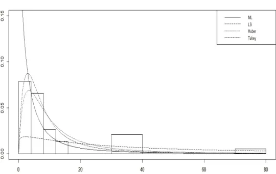
5.1. Failure Time Data Set. Failure time data set has been considered by [4] to illustrate the performance of the proposed robust estimators for the parameters of the Burr XII distribution and by [5] to illustrate the proposed Optimal B-robust estimators for the parameters of the Burr XII distribution. The data set has been also used by [20] to illustrate the potential of the Burr XII power series distribu-tions. The data set contains the failure times of 20 mechanical components. The parameter estimations obtained from the ML, LS and proposed robust estimation methods are given in Table 7.
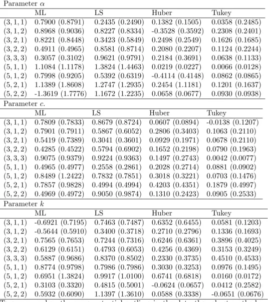
Table 7 Parameter Estimations for the Failure Time Data Set
b bc bk
ML 1.3060 1.7359 32.9140 LS 3.0968 2.1149 96.3755 Huber 2.6637 2.0053 108.6202 Tukey 2.4360 2.0651 152.436
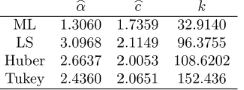
The …tted pdfs and histogram of the failure time data set are given in Figure 2. From Figure 2, we can observe that the data set contains a potential outlier. It has also been observed from Figure 2 that the ML and LS estimators are heavily distorted by this single outlier. However, the robust estimators do not seem very a¤ected by the outliers. In particularly, the robust estimator based on Tukey’s function provides better …t than the others in terms of modeling the data. We can observe that the …tted density obtained from Tukey seems summarizing data more accurant than the others. On the other hand, clearly the …tted density obtained from ML is a¤ected by the outliers and it is not provided a good …t to the data. It is not catching the pick of the data. It may be said that ML method is underestimating the parameters. The …tted density obtained from the robust estimator based on Huber’s function is also seem better than that of ML and LS …ts. In summary, the performance of the robust methods in terms of the …tting density to the data seems quite satisfactory.
5.2. Electrical Insulating Data Set. The electrical insulating data set has been already considered by [2] to illustrate the MOEBXII distribution. The data set is consist of electrical insulating described in [12] in which the lenght of the time until breakdown recorded. The data set is analyzed at 34 kilovolts with sample size n = 19 in this application. The ML estimation method is used to estimate the parameters of this distribution and the results are found as (4; 0:9; 1:002) in the paper by Al-Saiari et al. [2].
Figure 2. Histogram of the Failure Time Data Set and …tted densities Alternative to the ML estimator we use the LS and the robust estimation meth-ods proposed in this paper. We also recompute the ML estimate. The results are given in Table 8. Note that the ML estimator is very close to the estimate they have given. The other estimates are also close to the ML estimate. Note that to obtain LS and robust estimates we use the ML estimates given by [2] as the initial estimate for the algorithm.
Table 8Parameter Estimations for the Electrical Insulating Data Set with the initial values ( 0; c0; k0) =(4,0.9,1)
b bc bk
ML 4.003 0.91 1.0032
LS 6.865 0.6434 1.029
Huber 5.217 0.82 1.004 Tukey 5.924 0.932 1.432
Figure 3 shows the histogram of the electrical insulating data set and …tted pdfs obtained form ML, LS, Huber and Tukey according to Table 8.
From Figure 3, we can observe that all estimations of the parameters are closer to each other. However, the LS estimator seems to be more e¤ected by the potential outlier than ML and robust estimators. But the di¤erence of between the estimates
Figure 3. Histogram of the Electrical Insulating Data Set and …tted densities (( 0; c0; k0)=(4,1,1))
is not satisfactory enough to claim the superiority of the methods. To gain same more details about the data, we further use the kernel density estimation to see the overall …t to the data. We observe that the …tted densities instead of having L-shaped densities we may have unimodal skewed density. Therefore we taken di¤erent initial values for the algorithm such as ( 0; c0; k0) = (20; 1; 1) and end it
up with the di¤erent estimates for the parameters given in Table 9.
Table 9Parameter Estimations for the Electrical Insulating Data Set with the initial values ( 0; c0; k0) =(20,1,1)
b bc bk
ML 6.002 0.8364 1.4726
LS 51.184 1.19 0.8721
Huber 27.016 1.8721 0.8043 Tukey 23.043 1.8439 0.8727
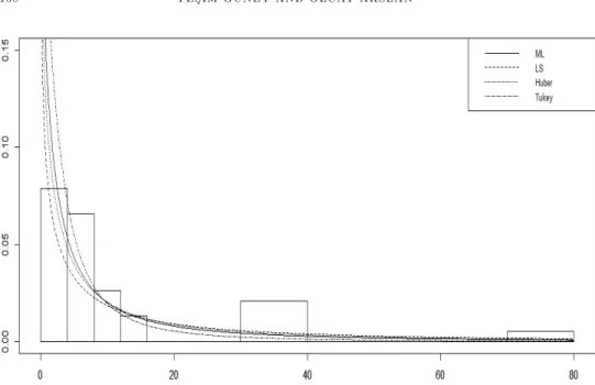
The histogram of the electrical insulating data set and …tted pdfs obtained form ML, LS, Huber and Tukey according to Table 9 are given in Figure 4.
Now, we can clearly observe that the LS estimator under…t the data. It can be seen that the …tted pdf obtain from ML estimator is still L-shaped. In such cases, it might be expected that the frequencies of the smaller values would be quite large,
Figure 4. Histogram of the Electrical Insulating Data Set and …tted densities (( 0; c0; k0)=(20,1,1))
and the frequencies of the larger values would be quite small. Therefore, the …tted density obtained from ML is not provided a good …t to the data. The …tted density obtained from the robust estimator based on Huber’s function is seem better than that of ML and LS …ts. Tukey would be preferable to …t this data set among others as in Failure Time Data Set example since it catch the pick better than the others.
6. Conclusion
In this study, alternative robust estimation methods based on M estimator have been proposed to obtain estimators for the parameters of the MOEBXII distribu-tion. We have compared the performance of these methods through a simulation study and real data examples. It is concluded that all the methods considered show identical performance for estimating the parameters of the MOEBXII distribution unless the data set contain outlier. However, the robust estimation methods per-form better for the data sets with outlier than ML and LS estimation methods. From both simulation study and real data examples, the e¤ect of outliers on the LS and ML estimates is fairly obvious. Therefore to eliminate the outliers’e¤ects, robust methods can be preferable. There are other robust estimation methods such as Optimal-B robust estimation that can be used to estimate the parameter of the MOEBXII distribution. This will be future work.
7. ACKNOWLEDGMENT
The authors would like to thank the Editor/referee for the valuable comments on our submitted manuscript.
References
[1] Al-Hussaini, E. K. and Jaheen, Z. F., Bayes Estimation of the Parameters, Reliability and Failure Rate Functions of the Burr Type XII Failure Model, Journal of Statistical Computa-tion and SimulaComputa-tion (1992), 41 (1-2), 31-40.
[2] Al-Saiari, A. Y., Baharith, L. A. and Mousa, S. A., Marshall-Olkin Extended Burr Type XII Distribution, International Journal of Statistics and Probability (2014); 3 (1), 78-84. [3] Burr, W., Cumulative Frequency Functions, The Annals of Mathematical Statistics (1942),
1 (2), 215-232.
[4] Dogru, F. Z. and Arslan, O., Alternative Robust Estimators for the Shape Parameters of the Burr XII Distribution, International Journal of Mathematical, Computational, Physical, Electrical and Computer Engineering (2015), 9 (5), 271-276.
[5] Dogru, F. Z. and Arslan, O., Optimal B-robust estimators for the parameters of the Burr XII distribution. Journal of Statistical Computation and Simulation (2016), 86 (6), 1133-1149. [6] Ghitany, M.E., Al-Awadhi, F.A. and Alkhalfan L.A., Marshall–olkin extended lomax
distrib-ution and its application to censored data, Communications in Statistics Theory and Methods (2007), 36 (10), 1855-1866.
[7] Gui, W., Marshall-Olkin Extended Log-Logistic Distribution and Its Application in Mini…-cation Processes. Applied Mathematical Sciences (2013), 7 (80), 3947-3961.
[8] Gupta, P.L., Gupta, R.C. and Lvin, S.J., Analysis of failure time data by burr distribution, Communications in Statistics-Theory and Methods (1996), 25, 2013-2024
[9] Hossain, A. M. and Nath, S. K., Estimation of parameters in the presence of outliers for a burr XII distribution, Communications in Statistics - Theory and Methods (1997), 26 (3), 637-652.
[10] Huber, P. J., Robust estimation of a location parameter, Ann. Math. Statist. (1964), 35, 73-101.
[11] Klugman, S. A., Loss Distributions. Proceedings of Symposia in Applied Mathematics Actu-arial Mathematics (1986), 35, 31-55.
[12] Lawless, J. F., Statistical Models and Methods for Lifetime Data. New York: John Wiley, 2003.
[13] Malinowska, I., Pawlas, P. and Szynal D., Estimation of location and scale parameters for the Burr XII distribution using generalized order statistics, Linear Algebra and its Applications (2006), 417 (1), 150-162.
[14] Marshall, A.W. and Olkin, I., A new method for adding a parameter to a family of distrib-utions with application to the exponential and weibull families, Biometrika (1997), 84 (3), 641-652.
[15] McDonald, J. B., Some Generalized Function for the Size Distribution of Income, Economet-rica (1984), 52 (3), 647-663.
[16] Moore, D. and Papadopoulos, A. S., The Burr Type XII Distribution as a Failure Model under Various Loss Functions, Microelectronics Reliability (2000), 40 (12), 2117-2122. [17] Papadopoulos, A. S., The Burr Distribution as a Life Time Model from a Bayesian Approach,
IEEE Transactions on Reliability (1978), 27 (5), 369-371.
[18] Rodriguez, R. N., A guide to Burr XII distribution, Biometrika (1977), 64, 129-134. [19] Shah, A. and Gokhale, D. V., On maximum product of spagings (mps) estimation for burr
xii distributions, Communications in Statistics- Simulation and Computation (1993), 22 (3), 615-641.
[20] Silva, R. B. and Cordeiro, G. M., The Burr XII power series distributions: A new compound-ing family, Brazilian Journal of Probability and Statistics (2015), 29 (3), 565-589.
[21] Tadikamalla P. R., A Look at the Burr and Related Distributions, Int. Stat. Rev. (1980), 48(3), 337-344.
[22] Wingo, D. R., Maximum likelihood methods for …tting the Burr type XII distribution to life test data, Biometrical Journal (1983), 25 (1), 77–84.
[23] Wingo, D. R., Maximum likelihood methods for …tting the Burr type XII distribution to multiply (progressively) censored life test data, Metrika (1993), 40, 203–210.
Current address : Ye¸sim Güney (Corresponding author): Ankara University, Faculty of Sci-ences, Department of Statistics 06100 Besevler ANKARA TURKEY.
E-mail address : [email protected]
Current address : Olcay Arslan: Ankara University, Faculty of Sciences, Department of Statis-tics 06100 Besevler ANKARA TURKEY.