C om mun.Fac.Sci.U niv.A nk.Series A 1 Volum e 67, N umb er 1, Pages 168–178 (2018) D O I: 10.1501/C om mua1_ 0000000840 ISSN 1303–5991
http://com munications.science.ankara.edu.tr/index.php?series= A 1
DIFFUSIVE REPRESENTATION OF A FRACTIONAL CONTROL USING ADAPTIVE PARTITIONING ALGORITHM
DJALIL BOUDJEHEM, BADREDDINE BOUDJEHEM, AND BELGACEM MECHERI
Abstract. This article presents optimal fractional control. This control is based on the property of the invariance of a fractional order di¤erential equa-tion. The problem formulation of the used control is expressed by di¤usive representation. The fractional control problem is described in a minimiza-tion form, where the global optimum represents the di¤usive realizaminimiza-tion of the controller. To determine the optimal fractional di¤usive control, an adaptive partitioning algorithm is used. As an application, we have chosen the control of a DC motor with uncertain parameters.
1. Introduction
The fractional operators become an interesting tool in the systems mathematical modeling and design, their use appeared strongly in di¤erent disciplines. Moreover, their convenient interest has been proved in the last decade. These operators are widely used in automatic control systems to construct robust fractional controllers like fractional P I or P D , ...etc. [1, 2, 3, 4, 5, 6].
In controlling uncertain dynamic systems, the use of robust control laws that are able to ensure the best compromise between performances and Robustness is highly required. In order to satisfy this requirement researchers used the fractional control as an alternative choice, where the concept of the robustness is based on the property of the invariance of the fractional di¤erential equation.
The fundamental property of this control is to preserve as much as possible, and on all the domain of uncertainty, the dynamic features imposed by the control of the nominal system, up to time scaling (or to frequency scaling). However, the use of fractional operators leads to some di¢ culties and problems, which come mainly from the fact that these operators are hereditary with singular kernels, and hence the numerical approximation becomes very di¢ cult and requires large memory storage capacities. To remedy these problems, the fractional control will be achieved by
Received by the editors: December 20, 2016, Accepted: May 16, 2017.
2010 Mathematics Subject Classi…cation. Primary 05C38, 15A15; Secondary 05A15, 15A18. Key words and phrases. Fractional system, fractional controller, di¤usive representation, op-timal control, Adaptive partitioning Algorithm.
c 2 0 1 8 A n ka ra U n ive rsity C o m m u n ic a tio n s d e la Fa c u lté d e s S c ie n c e s d e l’U n ive rs ité d ’A n ka ra . S é rie s A 1 . M a th e m a t ic s a n d S t a tis tic s .
using the di¤usive representation [9]. This representation allows the realization of the fractional operators in non-hereditary way using linear dynamical systems of di¤usive nature.[9]
We apply this concept to the control of a DC motor of which the transfer function is uncertain. The uncertainty is carried at the mechanical load and the current loop constant time. The non strict invariance consists in the minimization of an adequate cost functional. The optimal controller is achieved by using new algorithm so called ’Adaptive Partitioning Algorithms.
This article is organized as follows. Section 2 gives an overview on fractional order control systems and its realization by a irrational function . Section 3 de-scribes the principle of the control design. where the mathematical formulation of the optimal control are presented by di¤usive model. In section 4, we discuss an experimental design that is used to construct the new sub-regions and to generate the new populations. This design produces a set of individuals; each one occupies a subregion of the feasible region. Finally, an application are given in section 5
2. Fractional Calculus
In this part, We present some concepts of the fractional calculus, its scope and the di¢ culties associated with it. We also present the fractional operator realization using the di¤usive representation.
2.1. Fractional Operator. The fractional derivation and integration of order 2 [0+1] of a causal function f, formulated by Riemann-Liouville, is given by [1, 5, 6].
I (t) = Z 1 0 (t )( 1) ( ) f (t)d (2.1) Dtf (t) = d dt Z 1 0 (t ) (1 )f (t)d (2.2)
where is the gamma function de…ned by the expression: ( ) =R01t( 1)e tdt
2.2. Fractional systems. A linear fractional system with constant coe¢ cient can be represented by a fractional order di¤erential equation given by
K X k=0 ak d dt k y(t) = M X k=0 bk d dt k f (t) (2.3)
where K and M are integers, ak, bm are real numbers and k, k are arbitrary
constants.
Using Laplace transform of 2.3, we obtain the following transfer function H(s) = PM k=0bks k PK k=0aks k (2.4)
If there are k, l and m as ka = m:a1 and m= k 1, then the fractional system
(2.4) is called to commensurable order system, if this is not the case it is not a commensurable order.
2.3. Problems related to the fractional calculus. The di¢ culties encountered in the study of systems containing fractional operators, come mainly from the fact that these operators are hereditary with singular kernels, making the numerical approximation very di¢ cult and requires large memory storage.
2.4. Di¤usive Representation. The theory of di¤usive representation allows the realization of fractional operators in non-hereditary way using linear dynamical systems of di¤usive nature. It is very suited to the analysis and study of systems containing these operators.
Let H(s) be a transfer function (non-rational) associated with the causal convolu-tion operator H(d=dt), the di¤usive canonic realizaconvolu-tion of this operator is expressed, if any, by the realization of the state f ! y = h(d=dt)f = h f [10, 11].
@t'(t; ) = (t; ) + f (t)
y = R01 ( )'(t; )d (2.5)
where ( ) is called di¤usive representation of H(d=dt).
The di¤usive representation ( ) of an invariant symbol pseudo-di¤erential time operator H(s) is de…ned, if any, as the integral equation solution [7, 8].
H(s) = Z 1
0
( )
s + d (2.6)
Equation 2.6 is the transfer function associated with the di¤usive representation, with = L 1fhg, and h is the impulse response.
h(t) = Z +1
0
( )e td (2.7)
The di¤usive representation is therefore the use of the Laplace transform in the opposite direction , wherein t plays the role of the Laplace variable.
3. Fractional Control
3.1. Principle. Let’s consider the fractional di¤erential equation of order with uncertain parameter :
d
dt y (t) + y (t) = e (t) 1 < 2 (3.1)
The corresponding transfer function is given by:
H (s) = 1
s + 1 (3.2)
The system (3.2) is the closed loop transfer function of the open loop transfer function Holgiven by
Hol(s) =
1
s : (3.3)
The transfer function 3.3 is the Bode’s ideal transfer function where the gain crossover frequency !c is 11.
The transfer function given by (3.2) is closed to a damping second order transfer function, and the damping ration is related directly to and insensitive to gain variations [12] which give a time responses with iso-damping.
In mathematical point of view, the gain variations may be presented are equiva-lent to a change of time scale. Using the change of frequency ~s = 1s, the transfer function (3.2) will be written in the following form:
H (s) = 1
~
s + 1: (3.4)
All changes of the value of are equivalent to a change of frequency scale. In other way, the closed loop transfer function presents the property of the invariance under transformation noted T and de…ned by = 1 [13].
The set of changes of frequency de…ned by a function > 0 are a group of transformations under change of frequency [13]. We can write then:
(T H ) (s) = H ( s) = H 0(s) (3.5)
where 0 is the nominal parameter
3.2. Optimal fractional controller design. In control system, The system 3.3 may be used as a reference model to design a controller . In the case it is impossible to determine analytically a controller that permits to give a system closed to (3.3), the problem are solved through an optimization problem. So, the mathematical formulation of this problem are given by
min
C2 = (F (C) ; F (C0)) (3.6)
where F (C) is the closed loop transfer function of the uncertain system controlled by a fractional compensator C, and F (C0) is the desired closed loop transfer function
for the nominal system controlled by the classical controller C0.
In the problem described by (3.6), the functional cost under group of transfor-mation can be expressed in a Hilbert space as follows [14]:
min T2&;C2 n kT F (C) F 0(C0)k 2 ;s o (3.7) where & is the group of continuous functions de…ned on , is the space of con-trollers and k : k2
;s is the H2 Hilbertien norm. This formulation permits to get a
compensated transfer function with proximity to the reference response de…ned by a standard controllers C0 , where T F (C) is closed as possible to F 0(C0), 8 2 .
The transfer function of the optimal controller C (solution of the problem 3.7) are a rational function. So, the controller C is a fractional controller that can be
achieved via di¤usive representation given by (2.6). Therefore, The problem of minimization (3.6) can be formulated under di¤usive formulation by (3.8) [14].
min T2& ;Kminc2 n kT F (C ) F 0(C0)k 2 ;! o (3.8) where the compensator C (s) is de…ned by:
C (s) = Kc
Z +1 1
( )
s + d (3.9)
4. The optimization algorithm
In the optimization part we used an adaptive partitioning algorithm. The prin-ciple of this algorithm is based on successive division of the search space until a narrow area is achieved about the global optimum. The initial search space denoted by 0is partitioned into C2msub-regions denoted by i(i = 1::k), where t indicates
the iteration number and m is the number of the best points selected after sampling the initial search space. m is de…ned at the beginning of the optimization operation. The partitioning and sampling operations are established using new experimental technique that will be described in what follows.
4.1. The proposed experimental design. The proposed technique that we call "circular design" is an experimental technique that permits to generate a set of points (individuals) around a central point expected to be the global optimum located between two points (that we called "parents") Xt
P 1and XP 2t [15, 16]. These
individuals are selected form a population that occupies a limited region in the search space. The new population has a property that the point’s distribution density decreases when we go far from its center (the expected global optimum). This is due to the fact that the points’ distribution should have higher density about the central point.
To illustrate the proposed idea, let’s suppose an n dimensional problem, thus at an iteration time t, a population of q individuals can be generated from two individuals XP 1t and XP 2t . This population is located inside a hypersphere centered at Xct= [xtc1; xtc2; :::xtcn] (4.1) where: Xct= 1 2(X t p1+ Xp2t ) (4.2)
The coordinates of each individual Xt
k = [xtk1; xtk2; :::; xtkn] for (k =1,. . . , q), are
calculated using the system equation 4.3. 8 > > > > > > > < > > > > > > > : xtk1= xtc1+ R 2 n Y l=2 cos l xtkn= xtcn+ R 2 lsin 2and xtkr = xtcr+ R 2 n r+1Y l=2 cos l ! sin n r+2 (4.3)
for : r = 2; :::; (n 1) and k = 1; :::; q. and
l=
2
q ud(j; l)l = 1; ::; n (4.4)
Eq. 4.3 represents the circular transformation of ud = [udij]q n, a matrix of points
uniformly scattered and is obtained by applying the linear uniform design technique discussed in [15, 16] over the considered research space. R is the radius of the hypersphere and is given by (4.5).
R = q
(Xt
P 1 XP 2t )T(XP 1t XP 2t ) (4.5)
Equation 4.5 shows that the error o¤set equals to 1=2 of the population radius i.e. the real selected sub-region 0i(t) to be repartitioned at iteration t + 1 is greater than i(t). Hence, we reduce the probability to miss the global optimum, supposing
that i(t) is the most promising subregion and contains the global optimum.
The proposed experimental technique mechanism is summarized as follows: At each iteration number t, we generate Cm
2 populations; each population
oc-cupies a sub-region of the search space; and each population is de…ned by its own vector Xt
k;i=1::ni, where ni = 1::C2m. We should notice that the space includes Xit
represents exactly i.
The following de…nition describes the partitioning scheme of the APA.
De…nition. The collection of the sub-sets generated by the circular design at the iteration time t is de…ned as follows
S = f i; i = 1:::kg (4.6)
where k = C2m, and
f 1(t + 1) [ 2(t + 1) [ 3(t + 1)::: k(t + 1) \ i(t)g 6= (4.7)
The last equation shows that the union of the new produced sub-regions is greater than their parent region, which means that the set S does not represent an exact partition of i(t). The left side of the last relation describes the set that has a weak
probability of the global optimum existence. The real new sub-regions are given by a modi…ed sub regions denoted by 0
of the selected sub-region i(t + 1). Where 0
i(t + 1) = i(t + 1): i(t + 1) (4.8)
where i(t + 1) represents an error margin coe¢ cient which depends strictly on the parameters of a given sub region. This coe¢ cient allows the algorithm to reallocate the new sub-regions when the expected localization of the global optimum at iteration t do not con…rm those given by the stochastic tests at the iteration t+1. 4.2. The potential of a sub region and the decision factor. The way deciding which i(t) containing the global optimum is based on the sub-regions’potential.
The potential of a space can be evaluated using interval, and statistical estimation techniques [15] or fuzzy approaches [16]. For the fuzzy approaches, the degree of a membership of any point is measured by the membership function i;k of the function to minimize f (xij), xij 2 Di(t), and Di(t) represents a sample set of
the sub-region 0i(t). For the evaluation of i;k, several formulations are possible,
we can mention the S-membership function, the Gaussian membership function or the linear membership function. In this paper, we have chosen to compute i;k, using the modi…ed linear membership function, described in [15]. This member ship function maps sample points functional values f (xij) in 0i(t) to a unit interval
[0; 1].
t;ij= (f (xij) f (x ))=R(t) (4.9)
where f (x ) is the best (minimum) functional value obtained, and R(t) is the range of all functional values gathered up to and including the iteration t. the member ship function measures the location of f (xij) on the rang scale. Now, we can de…ne
the potential of a sub region using (4.10). rij = 1 q q X j=1
t;ij: exp(1 t;ij) (4.10)
q is the size of the sample set Di(t).
It is very important to mention here that the circular design forces the sub region, whose central point is located at the nearest position to the global optimum to have the smallest potential value by ensuring a good point distribution around this expected optimum. Thus, we ensure that the probability of missing the global optimum when t the iteration time increases goes to zero.
5. Application to a dc motor control
The open loop uncertain transfer function of the motor can be written as
H (s) = 1
J s (1 + Tbcs)
(5.1) The uncertainty is carried at the moment of inertia J "motor + load", the time constant Tbcof the current loop or on the two at the same time.
Let’s consider the nominal parameter 0which contains the nominal values of J
and Tbc noted by J0 and Tbc0 respectively. Where J is the moment of inertia. We
can distinguish three possible cases:
(1) 0= [J ], the moment of inertia J is uncertain and the constant of time Tbc
is …xed where: = [J0] [Tbc0].
(2) 0= [J0; Tbc], Tbc is uncertain, J is …xed where: = [J0] [Tbcmin; Tbcmax]
(3) 0= [J; Tbc] ; J and Tbcare uncertain where: = [Jmin; Jmax] [Tbcmin; Tbcmax]
We consider that the moment of inertia, the load and the time constant in the current loop are uncertain.
In this case it is impossible to …nd a compensator that confers a transfer function to the uncertain system of the form given by 3.9. Therefore, it is necessary to choose the best group of transformation that is well adapted to the chosen application that permits to have some invariant responses.
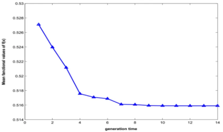
Figure 1. Mean functional values of the minimization problem of equation (3.9)
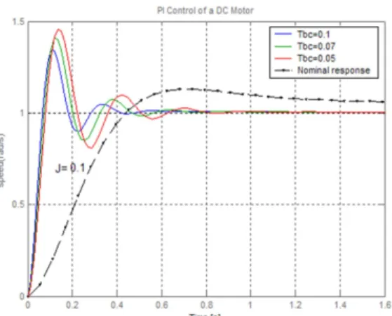
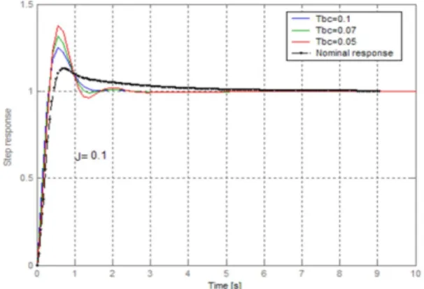
We used the proposed optimization algorithm to …nd out the optimal fractional corrector. The variations of the mean functional values are shown in …gure 1. Table 1 shows the center and the radius of the selected subregions during the optimization operation. Figures 2 and 3 present the step responses of the velocity for di¤erent values of Tbc, where, J=0.1 in the case of a classical PI controller and a fractional
one. It is very clear, that the fractional controller use permits to obtain pseudo invariant responses around nominal system response.
6. Conclusion
In this paper, optimal fractional control realization via di¤usive representation is proposed. The use of the di¤usive representation of pseudo di¤erential operators
Table 1. The center and the radius of the selected subregions The Center xm R(t ) t -1.3115 -7.3770 -0.8476 -6.3604 -0.7711 -5.9313 -0.6957 -5.5377 -0.6846 -5.4650 -0.7045 -5.0592 -0.6979 -5.0091 -0.6958 -4.9579 -0.6956 -4.9571 2.8013 1.8702 1.1871 0.5019 0.4043 0.1495 0.0632 0.0013 0.0006 1 2 3 4 5 8 9 13 14
Figure 2. Step response with classical PI controller
allow to solve a number of problems involving fractional operators or more generally long memory non oscillating ones by transforming them into input-output well posed di¤erential equations. The optimal solution obtained using the Adaptive partitioning algorithm was able to produce a stable controlled system with iso-damping step responses over the uncertainty domain of system parameters.
Figure 3. Step response with fractional controller
References
[1] I. S. Jesus, J. A. T. Machado, “Fractional control of heat di¤usion systems”. Nonlinear Dynamics, 54 (3), 263–282, 2008.
[2] D. Boudjehem, and B. Boudjehem. "A fractional model predictive control for fractional order systems." Fractional dynamics and control. Springer New York, 2012. 59-71.
[3] D. Boudjehem, and B. Badreddine. "Robust Fractional Order Controller for Chaotic Sys-tems." IFAC-PapersOnLine 49.9 (2016): 175-179.
[4] B. Boudjehem, and D. Boudjehem. "Fractional PID Controller Design Based on Minimizing Performance indices." IFAC-PapersOnLine 49.9 (2016): 164-168.
[5] D. Boudjehem, B. Boudjehem, “A fractional model for robust fractional order Smith predic-tor”. Nonlinear Dynamics, 73 (3), 1557–1563, 2013.
[6] B. Boudjehem, D. Boudjehem, “Fractional order controller design for desired response”. Pro-ceedings of the Institution of Mechanical Engineers, Part I: Journal of Systems and Control Engineering, 227 (12), 243–251, 2013.
[7] G. Montseny. “Simple Approach to Approximation and Dynamical Realization of Pseudo-di¤erential Time Operators such as Fractional ones”, IEEE Transactions on Circuits and Systems II, 51 (11), 613–618.
[8] G. Montseny, Di¤ usive representation of pseudo-di¤ erential time-operators. LAAS, 1998. [9] G. Montseny, “Di¤usive wave-absorbing control: Example of the boundary stabilization of a
thin ‡exible beam”. Journal of Vibration and Control, 18 (11), 1708–1721, 2012.
[10] L. Laudebat, P. Bidan, G. Montseny, “Modeling and Optimal Identi…cation of Pseudodif-ferential Electrical Dynamics by Means of Di¤usive Representation”, IEEE Transactions on Circuits and Systems I, 51 (9), 1801–1813, 2004.
[11] C. Casenave, G. Montseny, “Identi…cation and state realisation of non-rational convolution models by means of di¤usive representation”, Control Theory and Applications, IET, 5 (07), 934–942, 2011.
[12] Oustaloup, A. La commande CRONE: commande robuste d´ ordre non entier 1991, Hermès, Paris.
[13] Audounet, J., Devy-Vareta, F., and Montseny, G. Pseudo-invariant di¤usive control. In 14th Symosium of mathematical theory of networks and systems, perpignan, France, 2000.
[14] Devy-Vareta, F., Audounet, J., Matignon, D., and Montseny, G. Pseudo invariant by matched scaling: application to robust control of ‡exible beam. In 2nd European conference on struc-tural control, France, 2000.
[15] D. Boudjehem, B. Boudjehem, A. Boukaache. “Reducing dimension in global optimization”. International Journal of Computational Methods, 8 (03), 535–544, 2011.
[16] Boudjehem, Djalil, and Nora Mansouri. "A two phase local global search algorithm using new global search strategy." Journal of Information and Optimization Sciences 27.2 (2006): 425-436.
Current address : Djalil Boudjehem: Advanced Control Laboratory, Department of Electronics and Telecommunication, University of Guelma, ALGERIA.
E-mail address : [email protected]
Current address : Badreddine Boudjehem: Advanced Control Laboratory, Department of Au-tomatics and Electrotechnics, University of Guelma, ALGERIA.
E-mail address : [email protected]
Current address : Belgacem Mecheri: Advanced Control Laboratory, Department of Electronics and Telecommunication, University of Guelma, ALGERIA.