COMPARISON OF GROSS
CALORIFICVALUEESTIMATIONOF TURKISH
COALSUSING REGRESSIONANDNEURAL
NETWORKS TECHNIQUES
A Murat Ozbayoglu
1,*, M Evren Ozbayoglu
2and Gulhan Ozbayoglu
3,
ABSTRACT
Gross calorific value (GCV) of coals was estimated using artificial neural networks, linear and non-linear regression techniques. Proximate and ultimate analysis results were collected for 187 different coal samples. Different input data sets were compared, such as both proximate and ultimate analysis data, and only proximate analysis data and only ultimate analysis data. It was observed that the best results were obtained when both proximate analysis and ultimate analysis results were used for estimating the gross calorific value. When the performance of artificial neural networks and regression analysis techniques were compared, it was observed that both artificial neural networks and regression techniques were promisingly accurate in estimating gross calorific values. In general, most of the models estimated the gross calorific value within ±3% of the expected value.
Keywords: lignites, gross calorific value, proximate analysis, ultimate analysis, regression, neural networks
INTRODUCTION
Coal is a naturally occurring combustible sedimentary rock which is composed mostly of organic compounds and inorganic mineral matter and moisture. It is the most abundant fossil fuel and important source of energy for the present and future. Coal is classified according to its relative content of elemental carbon. Coal is further characterized according to heat (calorific) values, considered to be one of its most important properties, from a commercial or industrial aspect. Both of them are rank parameters.
Calorific value or heat content (energy value) is defined as the amount of heat evolved when a unit amount of coal is completely burnt and the products of combustion cooled to a standard temperature of 298 ºK. GCV assumes all vapor produced during the combustion process is fully condensed. The net calorific value is calculated from the gross calorific value (at 20 degree C) by making a suitable subtraction (572 kcal/kg= 2.395 MJ/kg) to allow for the water originally present as moisture as well as that moisture formed from the coal during the combustion. Calorific value is given in kcal/kg or kJ/kg. Power plant coals have a calorific value in the range of 9.5 MJ/kg to 27 MJ/kg (Zactruba, 2009).
The calorific value of coal varies considerably depending on the ash, moisture content and the type of coal. The calorific value used in establishing the rank of a coal is its gross calorific value which is determined experimentally by ASTM methods in a bomb calorimeter (ASTM Designation 1985a; 1985b). Alternative method for the direct
1. TOBB University of Economics and Technology, Department of Computer Engineering, Sogutozu Cad. No 43, Sogutozu, 06560 Ankara,
Turkey, [email protected]
2. The University of Tulsa, Department of Petroleum Engineering, Tulsa, OK, USA, [email protected]
determination of GCV of coals is by Differential Scanning Calorimetry (DSC) which was introduced by Fyans in 1977 (Fyans, 1977).
When a bomb calorimeter may not be available, the calorific value can be predicted from its chemical composition. Estimation of calorific value from the composition of fuel is one of the basic steps in performance modeling and calculations on thermal systems (Channiwala and Parikh, 2002).
Chemical composition of the coal is determined by proximate and elemental analyses. The proximate analysis consists of determination of moisture, ash, volatile matter and fixed carbon, while the elemental analysis comprises of qualitative determination of carbon, hydrogen, nitrogen, sulphur and oxygen. Various formulas which were based upon proximate and elemental analysis of coal as an input data are available for the prediction of calorific value (Kucukbayrak et al, 1991; Patel et al, 2007; Speight, 1994; Parikh, Channiwala and Ghosal, 2005; Mesroghli, Jorjani and Chelgani, 2009; Malhotra, 2010). They provide an easy and quick means for estimating the calorific value, thus saving the efforts involved in its experimental determination. Although these generalized correlations are useful, the elemental analysis input data should be provided which is obtained by the use of expensive equipment with highly skilled personnel. Therefore, the efforts are directed towards the estimation of calorific value of fuels from their proximate analysis.
The differential thermal analysis (DTA) can also be used for the determination of the calorific value of coal. Data obtained by the use of DTA are in good agreement with those obtained by the use of bomb calorimeter (Munoz-Guillena, Solano and Martinez de Lecea, 1992; Kok and Keskin, 2001).
The correlations which are based on proximate and/or elemental analysis are mainly linear in character, although there are indications that the relationship between the GCV and a few constituents of the proximate and elemental analyses could be nonlinear.A unified correlation for computation of GCV of solid, liquid and gaseous fuels has been established, using 225 data points. The correlation offered an average absolute error of 1.45% and bias error as 0.00% and thereby established its versality(Channiwala and Parikh, 2002). There are few correlations based on proximate analysis which is easy to perform and needs only standard equipments, but their use and applicability is limited to coal, or the region only (Kucukbayrak et al, 1991; Parikh, Channiwala and Ghosal, 2005; Cordero et al, 2001; Majumder et al, 2008; Ferguson and Rowe, 1986). Parikh, Channiwala and Ghosal (2005) introduced a general correlation, based on proximate analysis of solid carbonaceous materials like coals, biomass material and char. The average absolute error of this correlation was 3.74% and bias error was 0.12% with respect to the measured GCV.
Artificial Neural Networks (ANN) provides another methodology for nonlinear data prediction problems. Recently, researchers started working on developing different ANN models to estimate certain coal parameters and characteristics using experimental data. In one study, coal Hardgrove Index (HGI) estimation was implemented using several different regression and ANN models (Ozbayoglu, Ozbayoglu and Ozbayoglu, 2008). The results indicate the ANN methods were superior over the regression techniques in prediction performance. Patel et al (2007) developed a total of seven nonlinear artificial neural network (ANN) models for the estimation of calorific value of Indian coals. The results of the GCV estimation clearly suggested that all the ANN models possessed an excellent prediction accuracy and generalization performance with the comprehensive model that used all the major constituents of proximate and elemental analyses as inputs. Also, the ANN models estimated the magnitude of GCV with better accuracy than three linear models using the same inputs. The results also indicated that O, C, ash, fixed carbon and moisture have a stronger influence on the calorific value than volatile matter, He-density, N,H and S.
Works for the correlation of heating values with the chemical composition and the estimation of calorific values of Turkish coals from their proximate analyses are few. Urkan and Arikol(1989) estimated the heating value of 47
Turkish coals using proximate analysis. The results were comparable with the correlations based on elemental analysis. Kucukbayrak et al (1991) developed formulae by using 24 Turkish lignites to obtain calorific values from their proximate analysis. The correlations were based on least squares regression analysis. The mean differences between observed and calculated calorific values were in the range of 3.78% to 7.56%. Akkaya(2009) developed multiple nonlinear regression models for estimating higher heating value of low rank Turkish coals using proximate analysis. The best-fit model’s R2 was 0.97.
The aim of the present investigation is to predict the calorific value of Turkish lignites using both the proximate and elemental analyses of more than 187 samples, with the use of regression and artificial neural networks.
NEURAL NETWORKS
Artificial neural networks are used as universal function approximators in a wide range of applications. The most important aspect of neural networks is their ability to provide generalized solutions to highly nonlinear or “difficult-to-solve” problems where conventional methods such as regression or curve fitting do not perform well.
There are a variety of different neural network topologies, but multi-layer-perceptron (MLP) otherwise known as “backpropagation” is by far the most commonly used neural network type. MLP’s popularity comes from the fact that not only it is relatively easier to implement MLP for most problems, but also this particular neural network has outstanding generalization capabilities if configured and trained properly (Haykin, 1999).
MLP consists of an input layer, one or more hidden layers and an output layer. Each layer has a specified number of neurons which are fully connected to the neurons in the previous layer and the next layer, but not connected to the neurons in the same layer. The input features of the data points are fed into the input layer; hence the number of neurons in the input layer has to match the number of data features. However, in the hidden layer there is no constraint about the number of neurons or the number of hidden layers to be used. Even though there are various studies about the proper choice of number of hidden layers and neurons, there is a lack of evidence of a correlation between these parameters for a given problem. Most researchers use different MLP network configurations and observe the performance, so they can choose the topology that provides the best solution. The number of neurons in the output layer depends on the number of data parameters to be predicted in the system. Generally a single parameter is to be analyzed and predicted, but there are a lot of problems where several different parameters are needed to be forecasted, then the output data will be in a vector form. Also in most of the classification problems the neural network is configured so that it makes a selection from the output neurons each of which represents a particular class. In that case the number of neurons in the output layer will be equal to the number of classes in the problem.
This particular network structure is capable of finding generalized solutions to highly nonlinear problems and/or noisy data. The basic building block for MLP or any other neural network is the neuron, which by itself can be used as a general classifier or predictor; but for most problems it is not able to achieve satisfactory results due to its simplicity. However, for linearly separable classification problems, it is proven to converge to an acceptable result (Haykin, 1999).The neurons that are used in the backpropagation or MLP network differ from the original perceptron due to the introduction of the smooth nonlinear squashing function sigmoid instead of the hard nonlinear counterpart, the signum function, that was used in the original design of Rosenblatt in 1958 [20]. The basic reason for such a transformation was to be able to implement the gradient descent that was needed in the backpropagation learning algorithm (Rumelhart, Hinton and Williams, 1986).
Since most of the real-world problems have a high degree of nonlinearity by nature, and a single perceptron or neuron cannot handle such problems, MLPs and other neural network architectures that are based on the same concept of nonlinear mapping of the input space to the output space are introduced. These networks learn the input-output data pairs in such a way that the total error defined as the sum of squares of the difference between
the desired response (expected result) and the network output (actual result) is minimized. However, it is crucial to learn a general solution to the problem, not to overfit the input-output data, so that when new data is arrived, the neural network implementation will provide a satisfactory answer. This is achieved by using a cross validation (CV) data during the training stage. Actually, the cross validation data is not part of the training data, the network does not even know that particular data exists, but its performance (expected result – actual response) is measured while the neural network is tuning itself by changing the network weights. The most common approach is to continue on the training process as long as the cross validation error keeps going down. When CV error starts incrementing, or when it goes below an acceptable threshold level, then the training needs to stop in order to prevent overtraining of the network.
Linear and Nonlinear Regression
Linear regression is a forecasting or function approximation technique that aims to find the optimum line (or hyper-plane for higher input dimensions) that best represents the provided data points. The optimality in this particular problem is defined as minimizing the sum of squares of the difference of each individual data point from the linear regression hyper-plane. It is a widely used forecasting technique working well in highly correlated data. Nonlinear regression is based on the same principal approach used in linear regression, except the best representation of the data is not chosen as a hyper-plane, but as a nonlinear hyper-surface, and the level of nonlinearity depends on the input dimensions. Generally speaking, it can achieve better results when compared to linear regression, especially in nonlinear mapping problems.
MATERIALS AND METHODS
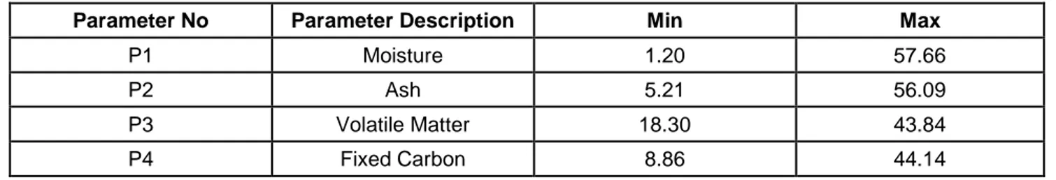
In this study, different coal samples collected from 187 coalfields which covers 110,000 km2 terrestrial Tertiary area in Turkey were used in predicting the gross calorific value for these coals. The total number of coal data points used in this analysis was 187 whose vitrinite reflectance (Rmax) varied between 0.312 and 0.782 and calorific value varied between 5.9 MJ/kg and 24.34 MJ/kg (Tuncali et al, 2002).The proximate analysis and ultimate analysis parameters used in the model are shown in Tables 1 and 2, respectively. During the regression calculations, kcal/kg was used as the heat unit, so the regression equations will give the equivalent result for MJ/kg.
Table 1Proximate analysis parameters used
Parameter No Parameter Description Min Max
P1 Moisture 1.20 57.66
P2 Ash 5.21 56.09
P3 Volatile Matter 18.30 43.84
P4 Fixed Carbon 8.86 44.14
Table 2Ultimate analysis parameters used
Parameter No Parameter Description Min Max
U1 Combustible Sulphur 0.01 10.29 U2 Total Sulphur 0.21 10.65 U3 Carbon 14.31 61.42 U4 Hydrogen 1.21 4.31 U5 Nitrogen 0.15 3.28 U6 Oxygen 0.79 23.16
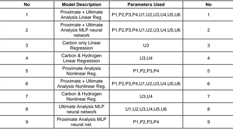
In this study, 9 different prediction models using linear and nonlinear regression techniques and MLP neural network using different combinations of proximate and ultimate analysis parameters were tested and compared. These models are shown in Table 3.
Table 3Prediction models used in this study
No Model Description Parameters Used No
1 Proximate + Ultimate
Analysis Linear Reg. P1,P2,P3,P4,U1,U2,U3,U4,U5,U6 1
2
Proximate + Ultimate Analysis MLP neural
network
P1,P2,P3,P4,U1,U2,U3,U4,U5,U6 2
3 Carbon only Linear
Regression U3 3
4 Carbon & Hydrogen
Linear Regression U3,U4 4
5 Proximate Analysis
Nonlinear Reg. P1,P2,P3,P4 5
6 Proximate + Ultimate
Analysis Nonlinear Reg. P1,P2,P3,P4,U1,U2,U3,U4,U5,U6 6
7 Carbon & Hydrogen
Nonlinear Reg. U3,U4 7
8 Ultimate Analysis MLP
neural network U1,U2,U3,U4,U5,U6 8
9 Proximate Analysis MLP
neural net. P1,P2,P3,P4 9
In order to have a fair comparison of the prediction techniques, same training and testing data is used throughout the process for all models. The data is divided into 8 equal subsets by randomly selecting equal number of data samples from the coal data set. As a result, 5 subsets of 23 random samples and 3 subsets of 24 random samples are formed. Then, each subset is tested separately using all the mentioned techniques in Table 3 as k-fold (k=8) testing. As a result, all 187 data points are tested. Then, the test performance results are compared.
RESULTS AND DISCUSSIONS
k-fold cross validation and/or testing is a commonly used method when there is a lack of available data for separate testing. It also provides a framework for better generalization and higher accuracy (Blum, Kalai and Langford, 1999). In this model, 8 different models are constructed for each test subset and for each prediction model and their results are compared. As a result of this 8-fold testing, all available data is tested for each model.
At the same time a correlation analysis between input parameters and output parameters are performed in order to identify which parameters are correlated and how much they affect the output directly. The correlation analysis results between all the parameters are shown in Table 4. Input parameters are explained in detail in Tables 2, 3. Output parameter is GCV.
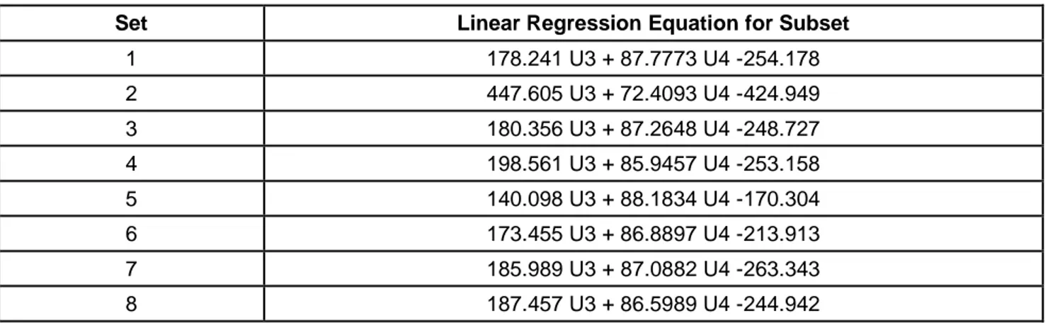
There are a total of 8 different linear regression equations for each training subset for each linear regression model. The best linear regression model is tabulated in Table 5.
Table 4Correlation analysis between each parameter P1 P2 P3 P4 U1 U2 U3 U4 U5 U6 GCV P1 1,0 -0,46 -0,4 -0,64 -0,29 -0,23 -0,64 -0,58 -0,44 0,07 -0,66 P2 1,00 -0,4 -0,32 0,16 0,15 -0,35 -0,31 0,02 -0,43 -0,33 P3 1,00 0,55 0,15 0,19 0,74 0,71 0,12 0,38 0,73 P4 1,00 0,14 0,03 0,94 0,81 0,53 0,21 0,94 U1 1,00 0,96 0,14 0,22 0,13 -0,53 0,20 U2 1,00 0,08 0,16 0,07 -0,53 0,13 U3 1,00 0,85 0,48 0,14 0,98 U4 1,00 0,34 0,15 0,87 U5 1,00 -0,24 0,47 U6 1,00 0,16 GCV 1,00
Table 5Linear regression parameters for Model 4, the best linear regression model
Set Linear Regression Equation for Subset
1 178.241 U3 + 87.7773 U4 -254.178 2 447.605 U3 + 72.4093 U4 -424.949 3 180.356 U3 + 87.2648 U4 -248.727 4 198.561 U3 + 85.9457 U4 -253.158 5 140.098 U3 + 88.1834 U4 -170.304 6 173.455 U3 + 86.8897 U4 -213.913 7 185.989 U3 + 87.0882 U4 -263.343 8 187.457 U3 + 86.5989 U4 -244.942
Quick analyses of the linear regression equations confirm coefficient similarities clearly indicating a regular data distribution over the subsets. Generally, data subset block #5 in all models show some discrepancies compared to other models since that this particular data block had more outliers compared to other blocks. The equations for the best nonlinear regression model are tabulated in Table 6.
Table 6Nonlinear regression parameters for Model 7, the best nonlinear regression model
Set Nonlinear Regression Equation for Subset
1 111.47 * U30.90327 * U40.1768 2 150.02 * U30.77201 * U40.35133 3 112.16 * U30.900486 * U40.178631 4 116.51 * U30.884947 * U40.195597 5 111.45 * U30.91312 * U40.140924 6 115.04 * U30.895604 * U40.171986 7 110.95 * U30.901777 * U40.182962 8 114.27 * U30.893294 * U40.185299
The neural network model used throughout this study is the Multilayer Perceptron (MLP). MLP network is well known for its generalization capabilities for nonlinear data problems [20]. Several different networks were developed and tested and the best results were achieved using a 2-hidden layer model, each having 20 neurons. Different networks having the same parameters but different weights were constructed by training each data set with 5000 epochs. Each neuron used sigmoid activation function. The learning algorithm was based on conjugate gradient method without momentum term. The network weights were updated and optimized based on minimum Cross Validation (CV) error.
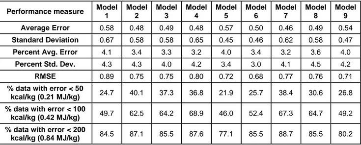
The results obtained from linear and nonlinear regression models and MLP neural network models are summarized in Table 7 where several different performance measures are evaluated.
Table 7 Performance analysis of the studied models
Performance measure Model 1 Model 2 Model 3 Model 4 Model 5 Model 6 Model 7 Model 8 Model 9 Average Error 0.58 0.48 0.49 0.48 0.57 0.50 0.46 0.49 0.54 Standard Deviation 0.67 0.58 0.58 0.65 0.45 0.46 0.62 0.58 0.47
Percent Avg. Error 4.1 3.4 3.3 3.2 4.0 3.4 3.2 3.6 4.0
Percent Std. Dev. 4.3 4.3 4.0 4.2 3.4 3.0 4.1 4.5 4.2
RMSE 0.89 0.75 0.75 0.80 0.72 0.68 0.77 0.76 0.71
% data with error < 50
kcal/kg (0.21 MJ/kg) 24.7 40.1 37.3 36.8 21.9 25.7 38.4 30.6 26.8 % data with error < 100
kcal/kg (0.42 MJ/kg) 49.7 62.5 64.2 68.9 46.0 52.4 67.3 64.7 49.2 % data with error < 200
kcal/kg (0.84 MJ/kg) 84.5 87.1 85.5 87.6 77.1 85.5 88.7 85.5 80.2
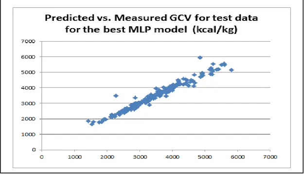
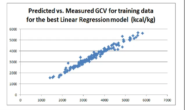
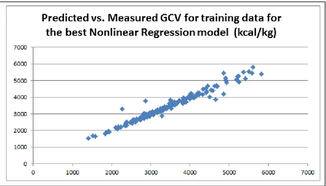
For each model and for each test subset, the average error is calculated. Average error is defined as the average of the absolute differences between the expected gross calorific result (obtained from the experimental data) and the generated output value from the model for each coal data in the particular test subset. In addition, the standard deviations of the model responses from the expected results are calculated. In order to have a scaled performance measure, the percent error calculations for both average error and standard deviation are also calculated. The prediction performances of the best models are also shown in Figures 1-7 where the training and test performance of the best linear regression, nonlinear regression and MLP models are presented.
Figure 1Predicted vs. Measured GCV test data using the best MLP Model (Model 2)
Figure 3Predicted vs. Measured GCV training data using the best Linear Regression Model (Model 4)
Figure 5Predicted vs. Measured GCV training data using the best Nonlinear Regression Model (Model 7)
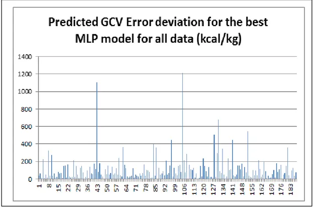
Figure 7Predicted GCV error deviation using the best MLP Model (Model 2)
The error deviation from the target GCV value (measured GCV) of the two best models are shown in Figure 6 and 7, where it was seen that most of the predicted data had relatively smaller deviation errors indicating, both models provided good generalization and predictions capabilities.
In another performance measure, a commonly used metric Root Mean Square Error (RMSE) (shown below) is also analyzed. Also in order to give a complete representation of the model performance, a basic output response distribution is demonstrated by indicating the percentage of the output values that have an error of less than 0.21, 0.42 and 0.84 MJ/kg respectively.
(1)
The results indicate that the best performance is obtained when linear or nonlinear regression is performed on carbon and hydrogen, which are the highest 2 correlated parameters with the gross calorific value; because, carbon, being a rank parameter has positive effect on gross calorific value while oxygen and moisture have negative effect. These results are tabulated in Tables 5 and 6 respectively. However, when all parameters are considered MLP neural network performed better than any other model (Table 7).
Implementing proximate analysis is much easier and faster compared to ultimate analysis. In order to take advantage of it, prediction models using only proximate analysis are also studied (Models 5 and 9). Once again, MLP neural network outperformed nonlinear regression neural network outperformed nonlinear regression even though the performance is not as successful as Models 2,3,4,6,7,8 where ultimate analysis results werepart of the input parameter vector.
In general most of the models estimated the gross calorific value within ±3% of the expected value. Model 2 (MLP neural network used with the both proximate and ultimate analysis) had the best prediction accuracy for the most amount of data points within a gross calorific value error of ±50 kcal/kg (±0.21 MJ/kg). More than 40% of the data points were within this range.
CONCLUSIONS
The results indicate the proposed models can be used in estimating the gross calorific value with an acceptable error rate. When outlier removal is performed, the performance increased significantly. Even though every tested model, more or less, can be used as an estimation model for GCV prediction, regression models in general slightly outperformed the neural network counterparts. This can be explained due to the fact that neural network models tried to learn the data regardless of how bad the data is, (assuming the outliers were experimentally problematic), whereas the regression models was mapping the data into a simpler output space. Using only proximate analysis also provided acceptable results, in that case the neural network model outperformed the regression model in both cases, so it did not change the outcome whether the full data was used or outliers were removed even though outlier removed helped the nonlinear regression estimator more than the neural network model. The percent error for the neural network estimator using only proximate analysis was 3.8% when the outliers were removed. In future work, fuzzy models might be added in order to handle the uncertainties in the data and the model parameters can be optimized using genetic algorithms.
REFERENCES
Akkaya,A V, 2009. Proximate analysis based multiple regression models for higher heating value estimation of low rank coals, Fuel Processing Technology90, pp165-170.
ASTM Designation D2015-85, Annual Book of ASTM Standards,05.21, 1985. ASTM Designation D3286-85, Annual Book of ASTM Standards,05.21, 1985.
Blum, A, Kalai, A, Langford, J, 1999. Beating the hold-out: bounds for K-fold and progressive cross-validation, Proceedings of the 12th Annual Conference on Computational Learning Theory, Santa Cruz, CA, USA, July 07-09 1999, pp 203-208.
Channiwala, S A, Parikh, P P, 2002. A unified correlation for estimating HHV of solid, liquid and gaseous fuels, Fuel 81, pp1051-1063.
Cordero, T, Marquez, F, Rodriguez-Mirasol, J, Rodriguez, J, 2001. Predicting heating values of lignocellulosic and carbonaceous materials from proximate analysis, Fuel 80, pp1567-1571.
Ferguson,J A, Rowe, M W, 1986. Calorific value of lignites from proximate analysis, ThermochimicaActa 107, pp291-298.
Fyans, R.L., 1977. Thermal Analysis Application Study,No:21, Perkin-Elmer Corp., Norwalk, CT.
Haykin, S,1999. Neural Networks: A Comprehensive Foundation, Second Edition, Prentice Hall, Upper Saddle River, NJ 07458 USA.
Kok, M V,Keskin, C, 2001. Calorific value determination of coals by DTA and ASTM methods, Journal of Thermal Analysis and Calorimetry Vol.64, pp1265-1270.
Kucukbayrak,S, Durus, B, Mericboyu, A E, Kadıoğlu, E, 1991. Estimation of calorific values of Turkish lignites, Fuel 70, pp 979-981.
Majumder, A K, Jain,R, Banerjee, P, Barnwal, J P, 2008. Development of a new proximate analysis based correlation to predict calorific value of coal, Fuel 87, pp3077-3081.
Malhotra, H, 2010. Calorific value of a fuel, http://www.economic expert.com/a/Calorific:Value:of:Coal.htm. Mesroghli, S H, Jorjani, E, Chelgani, S C, 2009. Estimation of gross calorific value based on coal analysis using
regression and artificial neural network, International Journal of Coal Geology 79, pp49-54.
Munoz-Guillena, M J, Solano, A L, Martinez de Lecea, C S,1992. Determination of calorific value of coals by differential thermal analysis, Fuel 71, pp579-583.
Ozbayoglu, G, Ozbayoglu, A M, Ozbayoglu, M E, 2008. Estimation of HardgroveGrindability Index of Turkish Coals by Neural Networks, International Journal of Mineral Processing 85 No:4, pp 93-100.
Parikh, J, Channiwala, S A, Ghosal, G K, 2005. A correlation for calculating HHV from proximate analysis of solid fuels, Fuel 84, pp 487-494.
Patel, S, Jeevan,K B, Badhe, Y P, Sharma, B K,Saha, S, Biswas, S, Chaudhury, A, Tambe, S S,Kulkarni, B D, 2007. Estimation of gross calorific value of coals using artificial neural Networks, Fuel 86 No.3 pp334-344. Rumelhart, D E, Hinton, G E, Williams, R J, 1986. Learning representations of back-propagation errors, Nature
vol. 323, pp533-536.
Speight, J G, 1994. The chemistry and technology of coal, 2nd ed. CRC Press, Taylor and Francis, p.181. Tuncali, E, Ciftci, B, Yavuz, N, Toprak, S, Koker, A, Gencer, Z, Aycik, H, Sahin, N, 2002. Chemical and
technological properties of Tersier age coal of Turkey, General Directorate of Mineral Research and Exploration, Ankara,Turkey, , ISBN: 6595-46-9, (Turkish).
Urkan, M K, Arikol,M, 1989. Correlations for the heating value of Turkish coals, Fuel 68No 4, pp527-530. Zactruba, J.,2009. Burning coal in power plants-Calorific value and