Applied genetic algortihms approach to curve fitting problems

(1)

T.C

BAHÇEŞEHİR ÜNİVERSİTESİ

APPLIED GENETIC ALGORTIHMS APPROACH TO

CURVE FITTING PROBLEMS

Master’s Thesis Sinem ŞENTÜRK

(2)

T.C

BAHÇEŞEHİR ÜNİVERSİTESİ

THE GRADUATE SCHOOL OF NATURAL AND APPLIED SCIENCES COMPUTER ENGINEERING

APPLIED GENETIC ALGORTIHMS APPROACH

TO CURVE FITTING PROBLEMS

Master’s Thesis

Sinem ŞENTÜRK

Supervisor: Prof. Nizamettin AYDIN

İstanbul, 2009

(3)

T.C BAHÇEŞEHİR ÜNİVERSİTESİ The Graduate School of Natural and Applied Sciences Computer Engineering Title of the Master’s Thesis : Applied Genetic Algorithms Approach to Curve Fitting Problems Name/Last Name of the Student: Sinem Şentürk Date of Thesis Defense : 02.09.2009 The thesis has been approved by the Graduate School of Natural and Applied Sciences. Assist. Prof. Tunç BOZBURA Acting Director This is to certify that we have read this thesis and that we find it fully adequate in scope, quality and content, as a thesis for the degree of Master of Science. Examining Committee Members: Prof. Nizamettin Aydın : Asc. Prof. Adem Karahoca : Assist. Prof. Orhan Gökçöl :

(4)

ii

ACKNOWLEDGEMENTS

I would like to specially thank to my supervisors Prof. Dr. Nizamettin Aydın and Asc. Prof. Dr. Yusuf Cengiz Toklu for their support, apprehension and unlimited tolerance during the course of this thesis.

(5)

ABSTRACT

APPLIED GENETIC ALGORTIHMS APPROACH TO CURVE FITTING PROBLEMS

Şentürk, Sinem Computer Engineering Supervisor: Prof. Nizamettin Aydın

September 2009, 30 pages

An alternative method was proposed for curve fitting in this study. The proposed method is Genetic Algorithms Method of which the application areas are getting wider recently. The application of Genetic Algorithms does not require auxiliary information and preliminary work as other parameter estimation methods. Therefore, it is practical for complex applications.

Within the scope of this study, a program was developed in order to show that it is possible to estimate the parameters of a simple polynome without requiring complex and long mathematical operations for the solution. Sample results of this program were also included.

Key words: Curve fitting, evolution, genetic algorithms, interpolation, least squares

method.

(6)

iv

ÖZET

EĞRİ UYDURMA PROBLEMLERİNE UYGULAMALI GENETİK ALGORİTMA YAKLAŞIMI

Şentürk, Sinem Bilgisayar Mühendisliği

Tez Danışmanı: Prof. Dr. Nizamettin Aydın Eylül 2009, 30 sayfa

Bu çalışmada eğri uydurma yöntemlerine alternatif bir yöntem önerilmiştir. Bu yöntem gün geçtikçe daha geniş kullanım alanlarına sahip olan Genetik Algoritmalar yöntemidir. Genetik Algoritmaların kullanımı diğer parametre tahmin yöntemleri gibi destekleyici bilgiler ve ön hazırlık gerektirmez. Bu nedenle, karmaşık uygulamalar için kullanışlıdır. Bu çalışmada basit bir polinomun parametrelerini tahmin etmek için çözümü uzun süren karmaşık matematiksel işlemlere gerek duyulmayabileceğini gösteren bir program yazılmıştır ve sonuçlarına yer verilmiştir.

Anahtar Kelimeler: Eğri uydurma, evrim, genetik algoritma, interpolasyon, en küçük

(7)

LIST OF TABLES

Table 1: One Point CrossOver ... 7

Table 2: Two Point CrossOver ... 7

Table 3: Data models with unknown parameters ... 26

Table 4: Data Sets ... 26

(9)

LIST OF FIGURES

Figure 1: chart of y= x2 -2x + 1 ... 19

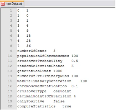
Figure 2: Data set and initial parameters ... 20

Figure 3: Output of the program ... 21

Figure 4: Estimated curve and original curve ... 21

(10)

viii

LIST OF EQUATIONS

Equation 1 ... 12 Equation 2 ... 12 Equation 3 ∑ ... 12 Equation 4 ∑ . ... 12 Equation 5 ∑ ∑ ∑ ; ... 13 Equation 6 ∑ ∑ ∑ … ∑ ∑ ∑ ∑ ∑ … ∑ ∑ ∑ ∑ ∑ … ∑ ∑ ∑ ∑ ∑ … ∑ … … … … ∑ ∑ ∑ ∑ … ∑ · … ∑ ∑ ∑ ∑ … ∑ ... 13

(11)

LIST OF ABBREVIATIONS

Genetic Algorithms : GAs

Average : AVG Deviation : DEV Genetic Algorithm : GA Chromosome : Chrom Probability of crossover : P (c) Probability of mutation : P (m) Probability of regeneration : P (r)

(12)

x

LIST OF SYMBOLS

Error :

Sum of square : Derivative of sum of square : ∂E Parameter which will be estimated : P

(13)

1 INTRODUCTION

One of the effective ways of defining the concept of a system is to create a mathematical model. In some circumstances, it may be required to build the mathematical model on the basis of data obtained from the systems through experimental approach. In such occurrences, the model is represented by limited number of samples.

The curve fitting algorithms use the limited number of data stacks in order to build the most appropriate mathematical model. With the help of this model they enable the computation of unknown values. However, the well-known curve fitting methods such as Gauss-Newton, Direct Search, and Variable Measurement Method may be time consuming in terms of their applications and necessary preliminary studies. These algorithms are generally suitable for a specific problem and may require restrictive assumptions related to continuity, existence of derivatives and any other limiting factors. Specific amount of auxiliary information is needed in order to have these algorithms to be used. If the starting point cannot be selected well, it may jam into local optimums and may provide only regional optimums. In such a case, the direction of the search may be altered and finding of the optimal results may be delayed.

In this study, Genetic Algorithms which doesn’t require auxiliary information and has an important role in solving the optimization problem were proposed for curve fitting. The structure of this study can be summarized in the following order:

Genetic algorithms and their operators are explained, The curve fitting operation is discussed,

The application developed with Java language for curve fitting using genetic algorithms was presented

(14)

2

2 GENERAL LITERATURE AND RESEARCH

INFORMATION

The main disadvantage of the parameter estimation methods, to produce solutions by using curve fitting, which have been effectively used within several areas such as from engineering to finance applications, from agriculture to information systems for several centuries, is that they cannot be used for all problems in general. There is a specific method for a specific problem available. Consequently, the researchers have been studying on Genetic Algorithms in order to provide a general solution to the problems. The curve fitting problems without using Genetic Algorithms can be sampled as the following:

Fitting closed form equations to data is useful for analysis and interpretation of the observed quantities. It helps in judging the strength of the relationship between the independent (predictor) variables and the dependent (response) variables, and enables prediction of dependent variables for new values of independent variables. Although curve fitting problems were first introduced almost three centuries ago (Stigler, S. M.

History of Statistics: The Measurement of Uncertainty Before 1900, Harvard University

Press, Cambridge MA, 1986), there is still no single methodology that can be applied universally. This is due to the diversity of the problem areas, and particularly due to the computational limitations of the various approaches that deal with only subsets of this scope. Linear regression, spline fitting and autoregressive analysis are all solution methodologies to identification and curve fitting problems.

There are several studies in literature in order to solve the curve fitting problems using Genetic algorithms.

Genetic Algorithms has been applied to system identification and curve fitting by several researchers. The relevant work on these can be categorized into two groups. The first one includes direct adaptation of the classical GA approach to various curve fitting techniques (Karr, C. L., Stanley D. A., and Scheiner B. J., “Genetic algorithm applied to least squares curve fitting,” U.S. Bureau of Mines Report of Investigations 9339, 1991.).

(15)

In these studies GA replaces traditional techniques as a function optimization tool. The second category includes much more comprehensive approaches where not only parameters of the model, but the model itself, are search dimensions. One leader work on this area is Koza’s adaptation of Genetic Programming (GP) to symbolic regression. The idea of genetically evolving programs was first implemented by (Cramer, N. L., “A representation for the adaptive generation of simple sequential programs,” Proceedings

of an International Conference on Genetic Algorithm and Their Applications, 183-187,

1985 and Fujiko, C. and Dickinson, J., “Using the genetic algorithm to generate LISP source code to solve prisoner’s dilemma,” Genetic Algorithms and Their Applications:

Proceedings of the Second International Conference on Genetic Algorithms, 236-240,

1987.). However, GP has been widely developed by Koza who has performed the most extensive study in this area. Recently, Angeline also used the basic GP approach enhanced with adaptive crossover operators to select functions for a time series problem (Angeline, Peter J., “Two self-adaptive crossover operators for genetic programming,”

Advances in Genetic Programming Volume II (editors: Peter J. Angeline and Kenneth E.

Kinnear, Jr.), MIT Press, Cambridge MA, 89-109, 1996.).

In this study, it was suggested with the help of outputs of the developed program that the Genetic Algorithms methods can be generally used as a solution in curve fitting problems supporting the researches mentioned and referenced above.

(16)

4

3 GENETIC ALGORITHMS

Genetic Algorithms (GAs) are adaptive heuristic search algorithms premised on the evolutionary ideas of natural selection and genetic.

The fundamentals of Genetic Algorithms were introduced by John Holland. They use two important features from natural evolution: handing down of information from one generation to another, or inheritance, and competition for survival, or survival of the fittest. The main advantages of GAs that make them suitable for solving real-life problems are:

• They are adaptive

• They possess inherent parallelism

• They are efficient for solving complex problems where the main focus is on obtaining good, not necessarily the best, solutions quickly

• They are easy to parallelize without much communication overhead

GAs are particularly suited for applications involving search and optimization where the space is huge, complex and multimodal and the need for finding the exact optimal solution is not all important (Bandyopadyay, S., Pal, S.K., 2007, Classification and

learning using genetic algorithms: applications in bioinformatics and web intelligence,

1, Springer, p.13).

There are several applications of Genetic Algorithms such as function optimization, tabulation, mechanical learning, design and cellular production. Unlike the global optimization methods, it uses the coded forms of parameters, not the parameter stack. Genetic Algorithms functioning according to the probability rules require the objective function only. They scan a particular area of the solution space, not the complete area. Thus, they provide quicker solutions by scanning the solution space effectively.

The scanning structure of the Genetic Algorithms is explained by sub-arrays theorem and structure blocks hypothesis. Sub-arrays are the theoretical structures used to explain

(17)

the behaviors of the Genetic Algorithms. Sub-arrays are defined by using the {0, 1, *} factors. The array below is a statement of the chromosome stack where the value of first position of the S sub-array is 0 and the second and fourth are 1. The value of the position shown as “*” could be either 0 or 1.

S = 01*1*

The degree and the length of sub-arrays, together form the essentials of the Genetic Algorithms. The degree of a sub-array is equal to the total number of constant positions in that sub-array. It is also equal to the sum of the total numbers of 0s and 1s.

The length of a sub-array is the distance from a specific initial position to the last position. Sub-arrays having consistent shortest length and lowest degree more than the population average are multiplied exponentially. This multiplication is realized with genetic operations and as a result, individuals having superior attributes and features than their parents are emerged. This provides a solution quality growing through generations.

Genetic Algorithms code each point within a solution space with binary bit array which is called chromosome. Each point has a fitness value. Genetic Algorithms deal with populations instead of single points. They form a new population in each generation by using genetic operators such as crossover and mutation. After a couple of generations later, the populations are consisted of individuals having better fitness values.

Genetic Algorithms includes forming of the initial population, computation of the fitness values, and execution of reproduction, crossover and mutation phases:

• Choose initial population • Repeat until terminated

o Evaluate each individual’s fitness o Prune population

(18)

6

Apply crossover operator Apply mutation operator

o Check for termination criteria (number of generations, amount of time, minimum fitness, threshold satisfied, etc.)

• Loop if not terminating

3.1. INITIALIZATION

Many individual solutions are randomly generated to form an initial population. The size of the population varies depending on the nature of the problem. The populations are formed with the members who are randomly selected from possible solution space.

3.2. FITNESS

A fitness value is computed for each individual within the population. There is a fitness function for each problem, for which a solution is searched. The fitness value plays an important role in selection of more proper solution in each generation. The greater the fitness value of a solution, the higher the possibility of its survival and reproduction.

3.3. SELECTION

The arrays are replicated according to the fitness functions in reproduction operator and individuals with better hereditary attributes are selected.

3.4. CROSSOVER

The crossover which is one of the operators affecting the performance of Genetic Algorithms corresponds to the crossover in natural population. Two chromosomes are randomly selected from the new population obtained as a result of reproduction operation and are put under a reciprocal crossover operation. In this operation where “L” is the length of the array, a “k” integer is selected within the “1 <= k <= L-1”

(19)

interval. The array is applied with a crossover operation based on the “k” value. The simplest crossover method is the single spotted / pointed crossover (Table 1) where both chromosomes need to be in same gene length.

Table 1: One Point CrossOver

In double spotted / pointed crossover the chromosome is broken in two points and the corresponding positions are replaced (Table 2).

Table 2: Two Point CrossOver

CROSSOVER POINTS 1 2 PARENT #1 0 1 2 3 4 5 6 7 8 9 PARENT #2 A B C D E F G H I J OFFSPRING A B 2 3 4 5 G H I J CROSSOVER POINTS 1 PARENT #1 0 1 2 3 4 5 6 7 8 9 PARENT #2 A B C D E F G H I J OFFSPRING 0 1 2 3 E F G H I J

(20)

8 3.5. MUTATION

If the population doesn’t contain the entire coded information, the crossover cannot produce an acceptable solution. Therefore, an operator capable of reproducing new chromosomes from the existing ones is needed. Mutation fulfills this task. In artificial genetic systems, mutation operator provides protection against the loss of a good solution which may not be re-obtained (Goldberg D.E. 1989, Genetic Algorithms in

Search, Optimization and Machine Learning, Addison-Wesley, USA). It converts a bit

value to another under a low probability value in the problems where binary coding system is used.

3.6. NEW POPULATION CREATION AND STOPPING THE OPERATION

The new generation will become the parent of the next one. The process continues with the fitness defined with the new population. This process continues until a defined number of populations or maximum iteration number or targeted fitness value is reached.

3.7. SELECTION OF PARAMETERS IN GENETIC ALGORITHMS

The parameters have significant impact on the performance of the Genetic Algorithms. Several studies were performed in order to find the optimal control parameters; however, no general parameters could be identified to be used for all problems (Altıparmak F., Dengiz B. ve Smith A.E., 2000, “An Evolutionary Approach For

Reliability Optimization in Fixed Topology Computer Networks”, Transactions On

Operational Research, Volume: 12, Number: 1-2, s. 57-75). These parameters are called as control parameters. The control parameters can be listed as:

• Population size, • Crossover probability, • Mutation probability, • Generation interval, • Selection strategy, and • Function scaling.

(21)

3.7.1. Population Size

When this value is too small, the Genetic Algorithm can jam into a local optimum. If the value is too great, the time needed to come to a solution becomes higher. In 1985, Goldberg suggested a population size computation method which is based on the chromosome length only. Furthermore, Schaffer and his friends expressed after researches and studies on several test functions in 1989 that a population size of 20-30 provides better results (Goldberg, 1985).

3.7.2. Crossover Probability

The purpose of the crossover is to create proper chromosomes by combining the attributes and features of existing good chromosomes. The chromosome couples are selected for crossover with P(c) probability. Increase in crossover operations causes increase in structure blocks; however, this also increases the probability of good chromosomes become spoiled.

3.7.3. Mutation Probability

The purpose of the mutation is to protect the genetic variety. The mutation can be occurred in each bit in a chromosome with P(m) probability. If mutation probability increases, the genetic search turns into a random search. However, this also helps to recall the lost genetic material.

3.7.4. Selection Strategy

There are several methods available to replace the old generation. In generation based strategy the chromosomes in the existing population are replaced with the children. Since the best chromosome in the population is also replaced it cannot be inherited to the next generation; therefore, this strategy is used together with the best fit / elitist strategy.

(22)

10

In best fit / elitist strategy, the best chromosomes in a population can never be replaced; therefore, the best solution for reproduction is always convenient.

In balanced strategy, only a few chromosomes are replaced. In general, the worst chromosomes are replaced when new ones are joined to the population.

(23)

4 CURVE FITTING

Curve fitting algorithms are used to build the most proper mathematical model based on limited amount of data.

The techniques developed to fit the curves to the data points are usually divided into two classes: Regression and Interpolation.

4.1. REGRESSION

This is used when there are distinctive errors regarding the data.

4.2. INTERPOLATION

This is used in order to identify the interim points between the data points where the related errors are ambiguous. It is simply defined as “the estimation of the values in blank fields using available numeric values”.

Interpolation is generally used in engineering and similar disciplines based on experiments / measurements in order to fit the collected data to a function curve.

It comes into prominence to identify the values in the blank fields using interpolation where the collected data is randomly distributed and particularly heterogeneous.

Interpolation techniques are generally applied by fitting the curve(s) to the available (xi, yi) data points. Various graded polynomials are used as Interpolation functions such

as logarithmic, exponential, hyperbolic and trigonometric functions (for periodic data values).

If the data points are distributed equal at intervals, it would be best to utilize interpolation techniques based on finite differentiation and if not, linear or LaGrange interpolation techniques would be the best option (Yükselen, M.A., HM504 Uygulamalı

(24)

12

In polynomial approach, only an “n = N-1 graded polynomial” can be passed through N number of points. Furthermore, an “N-1 graded polynomial” is passed through each data point.

Each co-efficient must be calculated in order to fit the curve to the data set where the data set is not linearly distributed. According to this, to have the polynomial

y = P0 + P1 * x + P2 * x2 + P3 * x3 + P4 * x4 + … + Pn * xn

the co-efficient i = {0, 1, 2, 3, 4, … , n} Pi must be calculated. There are “n + 1” numbers of unknown parameters in the problem.

By this definition:

Errors are calculated as:

Equation 1

Square of the errors is calculated as:

Equation 2

Sum of the squares is calculated as:

Equation 3 ∑

In order to obtain the smallest value of the sum of the squares, the derivates of E according to the Pi i = {0, 1, 2, 3, 4, …, n} parameters should be equal to zero:

(25)

The Pi co-efficient could be obtained by solving the “n+1” number of linear equations as achieved by the formula mentioned above. Thus, the equation system may be re-organized in different forms:

Equation 5 ∑ ∑ ∑ ; , , , , … ,

Another equation form:

Equation 6 ∑ ∑ ∑ … ∑ ∑ ∑ ∑ ∑ … ∑ ∑ ∑ ∑ ∑ … ∑ ∑ ∑ ∑ ∑ … ∑ … … … … ∑ ∑ ∑ ∑ … ∑ · … ∑ ∑ ∑ ∑ … ∑

(26)

14

5 GENETIC ALGORITHMS APPLICATION FOR

CURVE FITTING

The objective of curve fitting is to select functional coefficients which minimize the total error over the set of data points being considered. Once a functional form and an error metric have been selected, curve fitting becomes an optimization problem over the set of given data points. Since Genetic Algorithms have been used successfully as global optimization techniques for both continuous functions and combinatorial problems, they seem suited to curve fitting when it is structured as a parameter selection problem.

These points are the curve data which needs to be fitted by a polynomial equation. This sample data should fit an equation like

y = x2 -2x + 1

(x, y) = {(0, 1), (1, 0), (2, 1), (3, 4), (4, 9), (0, 15), (6, 25), (7, 36)}

First parameter is chromosome dimension which means number of genes, second parameter is represented the population of chromosomes, third parameter is crossover probability, fourth one is random selection chance % (regardless of fitness), fifth parameter represented the stop after this many generation, sixth one number of preliminary runs to build good breeding stock for final-full run, other parameter is maximum preliminary generations, eighth parameter is chromosome mutation probability - probability of a mutation occurring during genetic mating. For example, 0.03 means 3% chance, other parameters are crossover type, number of decimal points of precision, consider positive or negative float numbers, if true compute statistics else do not compute statistics.

(27)

T T g p A T c e t f f r To create a Two parents greater chan population d

After that fit

The ranking calculated. I example, if t the current fitness is low fitnessRank ranking num preliminary s are selecte nce of bein dimension. tness value f g of the pa If the fitness the fitness p generation, wer than any will equal t mbers denote

y population ed from pop ng selected.

for each mem

arameter "fi is high, the passed in is h the fitnessR y fitness valu to zero. The e very fit chr n, first of al pulation, wh The variab mber is comp fitness" with correspondi higher than a Rank will e ue for any ch e rankings fo omosomes. ll members here highly ble called “ puted: h respect to ing fitness r any fitness v equal to the hromosome i or all chrom must be sel fit individua “upperBoun o the curren anking will value for any e population

in the curren mosomes are

lected rando als were giv nd” value is nt generatio be high, too y chromosom nDim, and i nt generation calculated. omly. ven a s the on is o. For me in f the n, the High

(28)

16

Then the next generation of chromosomes is created by genetically mating fitter individuals of the current generation.

One point crossover on two given chromosomes:

Any duplicated genes are eliminated by replacing duplicates with genes which were left out of the chromosome.

For example, if we have:

chromosome A = { "x1", "x2", "x3", "x4" } chromosome B = { "y1", "y2", "y3", "y4" }

and we randomly choose the crossover point of 1, the new genes will be: new chromosome A = { "y1", "x2", "x3", "x4" }

new chromosome B = { "x1", "y2", "y3", "y4" }

Genetically the given chromosomes are recombined using a two point crossover technique which combines two chromosomes at two random genes, creating two new chromosomes.

For example, if we have:

chromosome A = { "x1", "x2", "x3", "x4", "x5" } chromosome B = { "y1", "y2", "y3", "y4", "y5" }

and we randomly choose the crossover points of 1 and 3, the new genes will be: new chromosome A = { "y1", "x2", "y3", "x4", "x5" }

(29)

Uniform crossover on two given chromosomes:

This technique randomly swaps genes from one chromosome to another. For example, if we have:

chromosome A = { "x1", "x2", "x3", "x4", "x5" } chromosome B = { "y1", "y2", "y3", "y4", "y5" }

uniform (random) crossover might result in something like: chromosome A = { "y1", "x2", "x3", "x4", "x5" }

chromosome B = { "x1", "y2", "y3", "y4", "y5" } if only the first gene in the chromosome was swapped.

When the elitism is employed the fittest two chromosomes always survive to the next generation. By this way, an extremely fit chromosome is never lost from the chromosome pool. In elitism the fittest chromosome automatically goes on to next generation (in two offspring):

this.chromNextGen[iCnt].copyChromGenes(this.chromosomes[this.bestFitnessChromIndex]);

The chromosomes previously created and stored in the "next" generation are copied into the main chromosome memory pool. Random mutations are applied where appropriate.

(30)

T s o p d The average smaller this optimal) sol population a different, the e deviation deviation, th lution. It cal are differen e higher the from the cu he higher th lculates this nt than the b deviation. 18 urrent popul he convergen s deviation b bestFitGene ation of chr nce is to a pa by determin s. The mor romosomes articular (bu ning how ma re the numb is obtained. ut not necess any genes in ber of genes The sarily n the s are

(31)

T t c t “ c The screen c tested with. column indi the solution “0, 1, 2, 3, 4 curve. 0,00 5,00 10,00 15,00 20,00 25,00 30,00 35,00 40,00 0 y capture belo The first co icates the “y of the polyn 4, 5, 6, 7” v

0,00 1,00

w (Figure 2) lumn repres y” value whi

nomial is “1 values. The c Figure 1 0 2,00 ) displays on ents the “x” ich satisfies 1, 0, 1, 4, 9, chart below 1: chart of y 3,00 4 y= x2_-2x ne of the pro ” value of the the “x” con 15, 25, 36” (Figure 1) d y= x2 -2x + 1 4,00 5,00 x + 1 oblems the a e polynomia ndition. It w ” where the “ displays the 1 0 6,00 applications al and the se was observed “x” variable “y= x2_-2x 7,00 8 were econd d that e gets + 1” 8,00

(32)

20

Figure 2: Data set and initial parameters

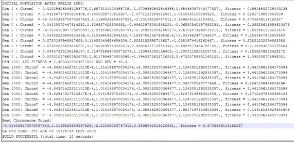
When the values above are provided to the program as input, the coefficients are obtained with an error rate of 0,009 within six (6) seconds. The member having the best fitness value out of 100.000 members resulted from a 1.000 generation where each generation produces 100 members, becomes the solution.

The solution or the coefficients of the curve in other words, for this sample has been found as:

P1 = 1.0003717114222255 P2 = -2.0030339280997236

(33)

T T f The function The curve w function abo 0,00 5,00 10,00 15,00 20,00 25,00 30,00 35,00 40,00 0 y n of the curv would be disp ove. 1 Figure 3 ve could be b y = 1.000 played as dep 2 : Output of built as follow 03*x2_{– 2.00} picted in fig 3 4 original estimate f the program ws (with fou 030x + 1.004 ure below (F 4 5 m ur decimal d 46 Figure 3) acc 6 digits): cording to th 7 he 8

(34)

I n a W f R T c T n It would be number of m also doesn’t When the d four parame Results after

The error rat calculated as The results w new populat e possible to members in mean that w ata set from ters, the foll r first run of

te for this sa s below:

were not eva tions and gen

o achieve b each genera we can obtain m the first sa lowing result f the program Figure 5 ample was 0 aluated as su nerations in 22 better and m ation and pr n better resu ample is app ts were obta m: : Output of ,232069 and P1 = 0.00 P2 = 0.87 P3 = -1.41 P4 = 0.25 ufficient and order to obta more accurat roviding gen ults with mor plied for a th ained (Figure f the program d the coeffic 83 32 137 27 d the process ain better res

te results by netic variety re members hird degree e 4): m ients of the p s is re-perfor sults (Figure y increasing y. However, and generati polynomial polynomial rmed by cre e 5). g the , this ions. with were ating

(35)

T p T P The error r polynomial w The polynom Program wa

ate for this were calcula

mial was solv as then re-exe Figure 6 sample red ated as below ved as “y = ecuted: : Output of duced to 0, w: P1 = 0.00 P2 = 0.97 P3 = -1.76 P4 = 0.64 -0.0010 * x3 f the program 162588972 10 32 628 49 3_{+ 0.9732 *} m and the co x2 - 1.7628 efficients of * x + 0.6449 f the 9”.

(36)

T t T T n I c T ( T

The error rat the polynom The polynom The accepta next trials. It It may be consecutive The error ra (Figure 7). T The paramet te for this sa mial were cal

mial was solv able results c

t should be n considered run in this s ate was furt The results ters were cal

Figure 7 ample reduce lculated as b ved as “y = could be obt noted that ev as coincid study. ther reduced were consid lculated as b 24 : Output of ed to 0,1296 elow: P1 = 0.01 P2 = 1.11 P3 = -2.20 P4 = 0.95 -0.0140 * x3 tained after very new run dence that w d to 0,07850 dered as acc below: f the program 656089 (Figu 40 69 015 96 3 + 1.1169 *

the first run n may not pr we obtained 09586 as als ceptable and m ure 6) and th x2 - 2.2015* n of the prog rovide better d better re so seen in th d the search he coefficien * x + 0.9596 gram or afte r results. sults after he output b was termin nts of 6”. er the each below nated.

(37)

T T The polynom The solution -6 -5 -4 -3 -2 -1 0 1 2 3 4 0 x

mial was solv

ns on the sam 1 2 ved as “y= -Figure 8 me platform 2 3 P1 = 0.00 P2 = 1.05 P3 = -2.01 P4 = 0.85 -0.0088* x3 + : Output of can be seen 4 88 99 154 83 + 1.0599* x2 f the program as below: 5 6 2 - 2.0154* x m 7 x + 0.8583” 8 first sec thir fou . t ond rd rth

(38)

26

6 EXPERIMENTAL RESULTS IN LITERATURE

It was observed that the results of the some experiments from the literature are parallel with the results of this study.

Table 3: Data models with unknown parameters

3 Parameter Functions

Gompertz

Logistic ⁄1

The data set obtained from Ratkowsky was used in parameter estimation for the functions from Table 3 (see Table 4 below).

Table 4: Data Sets

A B C

Y X Y X Y X

8.93 9 16.08 1 1.23 0 10.80 14 33.83 2 1.52 1 18.59 21 65.80 3 2.95 2 22.33 28 97.20 4 4.34 3 39.35 42 191.55 5 5.26 4 56.11 57 326.20 6 5.84 5 61.73 63 386.87 7 6.21 6 64.62 70 520.53 8 6.50 8 67.08 79 590.03 9 6.83 10 651.92 10 724.93 11 699.56 12 689.96 13 637.56 14 717.41 15

The GA control parameters in source are: • Population size, N = 60

• Number of maximum generations = 1000 • Re-generation probability, P (r) = 0.1

(39)

• Gene crossover probability, P (c) = 0.9 • Mutation probability P (m) = 0.01

The analysis was performed by GA for each given data set and the comparative results are listed in Table 5.

Table 5: Gauss-Newton and Genetic Algorithm application results

Gompertz Logistic

Data

Sets Parameters Gauss‐Newton GA Gauss‐Newton GA

A 82.830 82.730 72.46 72.534 1.224 1.224 2.618 2.612 0.037 0.037 0.067 0.067 3.630 3.636 1.34 1.344 B 723.1 722.75 702.9 700.56 2.500 2.503 4.443 4.444 0.450 0.451 0.689 0.689 1134 1133.9 744 744.17 C 6.925 6.9213 6.687 6.691 0.768 0.7696 1.745 1.764 0.493 0.4934 0.755 0.754 0.0619 0.0619 0.0353 0.035

Source: Ratkowsky, D.A., 1983, “Nonlinear Regression Modeling”, Marcel Dekker θ values were calculated with the formula θ S . Within this formula; n denotes the number of data pairs in a data set and p denotes the number of parameters in the regression equation.

The results show that the Genetic Algorithm method were calculated very close to the Gauss-Newton for a particular example as the results can be observed in Table 5.

(40)

28

7 CONCLUSION

The success of the optimization methods other than Genetic Algorithms depends on the initial point of the estimation. For instance, in order to determine the initial point when Gauss-Newton method is used for the search, a preliminary study is needed. In addition, some more information may also be needed regarding the function such as derivativeness and continuity of the variables.

As presented within this study, the Genetic Algorithms method does not need any auxiliary information and preliminary work. The researcher needs only to determine the generation number and population size and to set the mutation rate and crossover type. Such determination does not also require preliminary study. The acceptance rate of the problem, time and economical factors play decisive role. The researcher can accept the solution in any point of the time and terminate the operation.

The Genetic Algorithms differ from the other methods as it also provides solution population. All other methods focus on a single point of a search space. Therefore, the Genetic Algorithms can be used in parameter estimation of much more complex functions which make it a better alternative than other evolution based methods.

(41)

REFERENCES

Altıparmak F., Dengiz B. and Smith A.E., 2000, An evolutionary approach for

reliability Optimization in Fixed Topology Computer Networks, Transactions On

Operational Research, Volume: 12, Number: 1-2, s. 57-75

Altunkaynak, B., Alptekin, E., 2004, Genetic algorithm method for parameter

estimation in nonlinear regression, G.U. Journal of Science, 17(2):43-51.

Angeline, Peter J., 1996, Two self-adaptive crossover operators for genetic programming, Advances in Genetic Programming Volume II (editors: Peter J. Angeline and Kenneth E. Kinnear, Jr.), MIT Press, Cambridge MA, 89-109.

Bandyopadyay, S., Pal, S.K., 2007, Classification and learning using genetic

algorithms: applications in bioinformatics and web intelligence, 1, Springer, p.13.

Bäck, T. and Schwefel, H. P., 1993, An overview of evolutionary algorithms for

parameter optimization, Evolutionary Computation, 1, 1-23.

Cramer, N. L., 1985, A representation for the adaptive generation of simple sequential programs, Proceedings of an International Conference on Genetic Algorithm and Their

Applications, 183-187.

Fujiko, C. and Dickinson, J., 1987, Using the genetic algorithm to generate LISP source

code to solve prisoner’s dilemma, Genetic Algorithms and Their Applications:

Proceedings of the Second International Conference on Genetic Algorithms, 236-240. Goldberg D.E. 1989, Genetic Algorithms in Search, Optimization and Machine

Learning, Addison-Wesley, USA

(42)

30

Karr, C. L., Stanley D. A., and Scheiner B. J., 1991, Genetic algorithm applied to least

squares curve fitting, U.S. Bureau of Mines Report of Investigations, 9339.

Koza, J. R.,1992, Genetic Programming: On the Programming of Computers by Means

of Natural Selection, MIT Press, Cambridge MA, 162-169.

Ratkowsky, D.A., 1983, “Nonlinear Regression Modeling”, Marcel Dekker

Stigler, S. M., 1986, History of Statistics: The Measurement of Uncertainty Before

1900, Harvard University Press, Cambridge MA.

Wu, J., Chung, Y., 2007, Real-coded genetic algorithm for solving generalized

polynomial programming problems, Journal of Advanced Computational Intelligence

and Intelligent Informatics, Vol.11, No.4

(43)

CURRICULUM VITAE

Name Surname : Sinem Şentürk Birth Place / Year : İstanbul / 1981

Languages : Turkish (Native), English BSc : Bahcesehir University – 2006 MSc : Bahcesehir University – 2009 Name of Institute : Institute of Science

Name of Program : Computer Engineering Work Experience : 2008 May –

Software Developer

Anadolu Anonim Türk Sigorta Şirketi 2006 Sept – 2008 May

Teaching and Research Assistant

Bahcesehir University Computer Engineering Department

Applied genetic algortihms approach to curve fitting problems

T.C

BAHÇEŞEHİR ÜNİVERSİTESİ

APPLIED GENETIC ALGORTIHMS APPROACH TO

CURVE FITTING PROBLEMS

T.C

BAHÇEŞEHİR ÜNİVERSİTESİ

APPLIED GENETIC ALGORTIHMS APPROACH

TO CURVE FITTING PROBLEMS

Sinem ŞENTÜRK

Supervisor: Prof. Nizamettin AYDIN

ACKNOWLEDGEMENTS

ABSTRACT

ÖZET

TABLE OF CONTENTS

LIST OF TABLES

LIST OF FIGURES

LIST OF EQUATIONS

LIST OF ABBREVIATIONS

LIST OF SYMBOLS

1 INTRODUCTION

2 GENERAL LITERATURE AND RESEARCH

INFORMATION

3 GENETIC ALGORITHMS

4 CURVE FITTING

5 GENETIC ALGORITHMS APPLICATION FOR

CURVE FITTING

6 EXPERIMENTAL RESULTS IN LITERATURE

7 CONCLUSION

REFERENCES

CURRICULUM VITAE