Search for a W boson decaying to a vector-like quark and a top or bottom quark in the all-jets final state

CERN-EP-2018-279 2019/04/05

CMS-B2G-18-001

Search for a W

0

boson decaying to a vector-like quark and a

top or bottom quark in the all-jets final state

The CMS Collaboration

Abstract

A search for a heavy W0 resonance decaying to one B or T vector-like quark and a

top or bottom quark, respectively, is presented. The search uses proton-proton col-lision data collected in 2016 with the CMS detector at the LHC, corresponding to an

integrated luminosity of 35.9 fb−1 at √s = 13 TeV. Both decay channels result in a

final state with a top quark, a Higgs boson, and a b quark, each produced with sig-nificant energy. The all-hadronic decays of both the Higgs boson and the top quark are considered. The final-state jets, some of which correspond to merged decay prod-ucts of a boosted top quark and a Higgs boson, are selected using jet substructure

techniques, which help to suppress standard model backgrounds. A W0 boson

sig-nal would appear as a narrow peak in the invariant mass distribution of these jets. No significant deviation in data with respect to the standard model background

pre-dictions is observed. Cross section upper limits on W0 boson production in the top

quark, Higgs boson, and b quark decay mode are set as a function of the W0 mass,

for several vector-like quark mass hypotheses. These are the first limits for W0 boson

production in this decay channel, and cover a range of 0.01 to 0.43 pb in the W0 mass

range between 1.5 and 4.0 TeV.

Published in the Journal of High Energy Physics as doi:10.1007/JHEP03(2019)127.

c

2019 CERN for the benefit of the CMS Collaboration. CC-BY-4.0 license

∗_{See Appendix A for the list of collaboration members}

1

Introduction

Many extensions of the standard model (SM) predict new massive charged gauge bosons [1–

3]. The W0 boson is a hypothetical heavy partner of the SM W gauge boson that could be

produced in proton-proton (pp) collisions at the CERN LHC. Searches for W0 bosons have

been most recently performed at a center-of-mass energy of 13 TeV by the CMS and ATLAS Collaborations in the lepton-neutrino [4, 5], diboson [6, 7], and diquark [8, 9] final states. Vector-like quarks (VLQs) are hypothetical heavy partners of SM quarks for which the left- and right-handed chiralities transform the same way under SM gauge groups. Searches for VLQs have been performed by the CMS and ATLAS Collaborations in both the single [10–13] and pair

production [14–16] channels. The decay of the W0 boson to a heavy B or T VLQ and a top

or b quark, respectively, is predicted, e.g., in composite Higgs boson models with custodial symmetry protection [17–19]. These models stabilize the quantum corrections to the Higgs

mass and preserve naturalness. The W0 branching fraction to a quark and a VLQ depends

on the VLQ mass, with a maximum of 50% in the high VLQ mass range at the threshold of custodian production (see Ref. [20]).

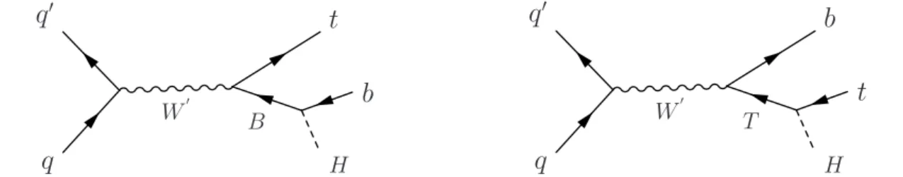
A search for a W0 boson in this decay mode is presented for the first time. The analysis consid-ers the decay channel where the B or T VLQ decays into a Higgs boson and a b or top quark, respectively, in the all-jets final state. Both the B and T VLQ-mediated decays result in the same

signature, as can be seen in Fig.1. Because of the high W0 and VLQ masses considered in this

analysis, the decay products are highly Lorentz boosted. These boosted decay products are reconstructed as single jets with distinct substructure, which is used in the analysis to

distin-guish them from SM multijet production. An inclusive search for a W0boson decaying to a top

quark, a Higgs boson, and a b quark is performed. The SM background is dominated by events comprised of jets produced via the strong interaction, referred to as quantum chromodynam-ics (QCD) multijet events, and top quark pair production (tt) events. These backgrounds are modeled by a combination of Monte Carlo (MC) simulation and control regions in data. The invariant mass distribution of the three-jet system, mtHb, is used to set the first limits on the W0

boson production cross section in the decay channel to a B or T VLQ. The data sample used in the analysis corresponds to an integrated luminosity of 35.9 fb−1[21] of pp collision data at

√ s=13 TeV, recorded in 2016. W0 _B

q

q

b

t

q

q

t

b

Figure 1: The W0 boson production and decays considered in the analysis. The analysis

as-sumes equal branching fractions for W0boson to tB and bT and 50% for each VLQ to qH.

The theoretical framework followed in the analysis is described in Ref. [20]. In this model the

top and W0 are superpositions of elementary and composite modes, with the top degree of

compositeness given by sL, and the mixing angle of the elementary and composite W0 states

given by θ2. The W0 boson production cross section is inversely proportional to cot2(θ2), but

low cot(θ2)values tend to be dominated by the leptonic W0boson decay mode. High values of

the sL parameter increase the relative phase space for the decay into two VLQs, whereas low

sLvalues enhance the W0 diboson decays. The analysis assumes this theoretical framework as

evaluated at sL =0.5 and cot(θ2) =3, which is chosen for the purposes of sensitivity in the W0

at 13 TeV using the framework of Ref. [20] for W0 masses in the range 1.5 to 4.0 TeV with the

assumptions that the W0 _→VLQ branching fraction is equally distributed between the tB and

bT final states. As a benchmark for the analysis, the VLQ branching fractions for each of the

decays B _→bH and T _→tH are assumed to be 50%, consistent with the benchmark used in

other recent searches.

2

The CMS detector

The central feature of the CMS apparatus is a superconducting solenoid of 6 m internal diame-ter, providing a magnetic field of 3.8 T. Within the solenoid volume are a silicon pixel and strip tracker, a lead tungstate crystal electromagnetic calorimeter (ECAL), and a brass and scintilla-tor hadron calorimeter (HCAL), each composed of a barrel and two endcap sections. Forward calorimeters extend the pseudorapidity coverage provided by the barrel and endcap detectors. Muons are detected in gas-ionization chambers embedded in the steel flux-return yoke outside the solenoid. A more detailed description of the CMS detector, together with a definition of the coordinate system used and the relevant kinematic variables, can be found in Ref. [22].

The particle-flow algorithm [23] aims to reconstruct and identify each individual particle with an optimized combination of information from the various elements of the CMS detector. The energy of each photon is obtained from the ECAL measurement. The energy of each electron is determined from a combination of the electron momentum at the primary interaction vertex as determined by the tracker, the energy of the corresponding ECAL cluster, and the energy sum of all bremsstrahlung photons spatially compatible with originating from the electron track. The energy of each muon is obtained from the momentum, which is measured by the cur-vature of the corresponding track. The energy of each charged hadron is determined from a combination of their momentum measured in the tracker and the matching ECAL and HCAL energy deposits, corrected for zero-suppression effects and for the response function of the calorimeters to hadronic showers. Finally, the energy of each neutral hadron is obtained from the corresponding corrected ECAL and HCAL energies that are not associated with a charged hadron track.

Jets are clustered with the anti-kT [24] algorithm in the FASTJET3.0 [25] software package. Jet

momentum is determined as the vectorial sum of all particle momenta in the jet, and is found

from simulation to be within 5 to 10% of the true momentum over the whole pT spectrum and

detector acceptance. Additional pp interactions within the same or nearby bunch crossings (pileup) can contribute additional tracks and calorimetric energy depositions to the jet mo-mentum. To mitigate this effect, charged particles originating from sub-leading pp collision vertices within the same or adjacent bunch crossings are discarded in the jet clustering proce-dure, where the primary collision vertex is defined as the vertex largest quadrature-summed

pT of all reconstructed particles. To account for the neutral pileup component, the pileup per

particle identification (PUPPI) algorithm [26] is used, which applies weights that rescale the jet transverse momentum based on the per-particle probability of originating from the primary vertex prior to jet clustering. Jet energy corrections are derived from simulation studies so that the average measured response of jets becomes identical to that of particle level jets. In situ measurements of the momentum balance in dijet, photon+jet, Z+jet, and multijet events are used to determine any residual differences between the jet energy scale in data and in simu-lation, and appropriate corrections are made [27]. Additional selection criteria are applied to each jet to remove jets potentially dominated by instrumental effects or reconstruction failures. The jet energy resolution amounts typically to 15% at 10 GeV, 8% at 100 GeV, and 4% at 1 TeV, to be compared to about 40, 12, and 5% obtained when the calorimeters alone are used for jet

clustering.

Events of interest are selected using a two-tiered trigger system [28]. The first level (L1), com-posed of custom hardware processors, uses information from the calorimeters and muon de-tectors to select events at a rate of around 100 kHz within a time interval of less than 4 µs. The second level, known as the high-level trigger (HLT), consists of a farm of processors running a version of the full event reconstruction software optimized for fast processing, and reduces the event rate to around 1 kHz before data storage.

3

Simulated samples

The tt production background is estimated from simulation, and is generated with POWHEG

2.0 [29–32]. The signal samples are generated at leading order using MADGRAPH5 aMC@NLO

2.3.3 [33, 34] with the NNPDF3.0 leading order parton distribution function (PDF) set, in the mass range from 1.5 to 4.0 TeV in 0.5 TeV increments. The analysis uses a QCD multijet

sam-ple as a cross check for the background estimate, which is also generated at LO with MAD

-GRAPH5 aMC@NLO. Parton showering and hadronization are simulated withPYTHIA8.212 [35]

using either the CUETP8M2T4 [36] or CUETP8M1 [37] underlying event tunes. For each W0

boson mass point, three VLQ mass points are generated with the VLQ mass range from 0.8 to

3.0 TeV. The generated VLQ masses are scaled to the W0 boson mass (m_W0) such that there is

a low (≈1/2 mW0), medium (≈2/3 m_W0), and high (≈3/4 m_W0) mass sample for each W0

bo-son mass point in order to explore the sensitive phase space of the boosted W0 boson decay

products. The generated W0boson and VLQ widths are narrow as compared with the detector

and reconstruction resolutions which is in accord with theoretical predictions for most of the

analyzed phase space. The simulation of the CMS detector uses GEANT4 [38]. All MC

sam-ples include pileup simulation and are weighted such that the distribution of the number of interactions per bunch crossing agrees with that observed in data.

4

Event reconstruction

The W0 → T/B → tHb channel is characterized by three high-pT jets. The jets from the top

quark (top jet) and Higgs boson (Higgs jet) decays tend to be wide and massive, whereas the jet from the b quark (b jet) will tend to be narrow and have a lower mass. Therefore, one jet clustered with the anti-kT algorithm with a distance parameter of 0.8 (AK8 jet) with pT >

300 GeV is required for the Higgs boson candidate jet. One AK8 jet with pT > 400 GeV is

required for the top quark candidate jet. One anti-kTjet with a distance parameter of 0.4 (AK4

jet) with pT >200 GeV is required for the b candidate jet. The separation∆R (

√

(∆φ)2_{+ (∆η)}2₎

between the two AK8 jets is required to be at least 1.8 in order to reduce the correlation of jet shapes arising from the abutting of jet boundaries, which can bias the background estimate. The AK8 jets are then selected as being consistent with a top quark or a Higgs boson decay using the tagging procedures defined below. The collection of jets considered for the b quark

candidate is then populated by AK4 jets with ∆R of at least 1.2 from the tagged AK8 jets.

In the case of multiple jets with the same tag, the tagged candidate is chosen randomly. Jet identification criteria are used for these three jets in order to reduce the impact of spurious jets from detector noise [39]. All jets in the analysis are required to be within|η| <2.4.

Because the signal of interest is a high mass resonance decaying to multiple high-pT jets, data

events are triggered by HT >800 or 900 GeV, where HT is defined as the sum of all AK4 jet

trigger requirement, and the AK8 jet pT trigger is included to overcome an issue in the trigger

HT calculation that impacts about 24% of the analyzed data.

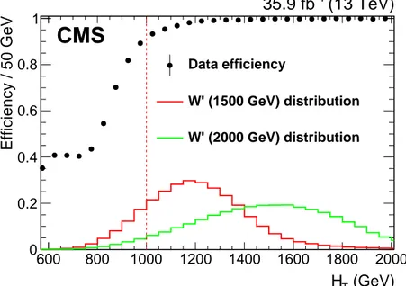
The efficiency of the trigger selection is studied using a sample of events that have at least one muon of pT>24 GeV. The fraction of these events that pass the full trigger selection is defined

as the trigger efficiency and is shown in Fig. 2 as a function of HT. The offline event selection

requires that HTbe larger than 1 TeV which ensures that the trigger efficiency is larger than 93%

near the threshold and is nearly 100% over most of the signal region. Although there is little inefficiency due to the trigger, this is taken into account as an event weight when processing MC samples. (GeV) T H 600 800 1000 1200 1400 1600 1800 2000 Efficiency / 50 GeV 0 0.2 0.4 0.6 0.8 1 Data efficiency W' (1500 GeV) distribution W' (2000 GeV) distribution

(13 TeV)

35.9 fb

CMS

Figure 2: Trigger efficiency as a function of HT. Events are required to have HT > 1 TeV as is

indicated by the red dashed line. The HTdistributions of two W0 signal hypotheses are shown

for comparison, normalized to unit area.

4.1 Top jet tagging

For top quarks with pT >400 GeV, the decay products, one b quark and two light quarks, can

merge into a single AK8 jet. Top quark jets are identified using a set of three quantities defined below.

The N-subjettiness [40] algorithm defines the τN variable, which quantifies how consistent the

jet energy pattern is with N or fewer hard partons, with the low τNvalues being more consistent

with N or fewer partons. In the case of a top quark hadronic decay, the ratio of τ3to τ2is used.

The merged top jet can also be discriminated from background by using the large top quark mass. The modified mass drop tagger algorithm [41], also known as the “soft drop” algorithm

[42] with β = 0 and z = 0.1 is used to calculate this mass variable, mt_SD. This algorithm

declusters the jet, and removes soft radiations, thus allowing a clearer separation between the merged top jet and background.

Finally, as the top jet contains a b quark, additional discrimination power can be achieved by using subjet b tagging with the combined secondary vertex version 2 (CSVv2) b tagging algorithm (SJcsvmax) [43]. We use a b tagging operating point defined by a 10% misidentification

The MC to data correction (scale factor) for the top tagging operating point in Table 1 is mea-sured to be 1.07+₋0.11_0.04in a sample enriched in semileptonic tt production, using the same proce-dure as outlined in Ref. [39].

4.2 Higgs jet tagging

In the case of a highly boosted Higgs boson in the bb decay mode, the decay products tend to merge into a jet that has a mass consistent with a Higgs boson and that contains two b hadrons clustered into the jet. Once again, the soft drop algorithm is used to provide the variable mH_SD as a measure of the Higgs boson jet mass, but in this case the jet is scaled using a simulation-derived correction suitable for resonances below the top jet tagging mass window [44], which is

pTand η dependent but results in a 5-10% mass amplification in both data and MC. Scale factors

are used for the jet mass scale and resolution, which are derived from a fit to the distribution

of the W boson jet mH

SDspectrum in a sample enriched in semileptonic tt production using the

technique outlined in Ref. [39].

To identify the two b quarks clustered into the merged Higgs jet, a dedicated double-b tag-ging algorithm (Dbtag) is used at an operating point with a misidentification probability of approximately 3% and an efficiency of 50%. Data samples enriched in QCD produced bb and tt events are used to establish scale factors for this tagger for the cases of signal and mistagged top quarks, respectively [43].

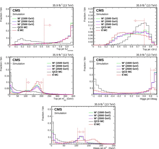
Figure 3 shows the variable distributions that are used for top and Higgs candidate jet tagging in tt, QCD, and signal MC simulation. The selections for these distributions includes all other top and Higgs candidate jet selections in order to preserve variable correlations.

In the rare occurrence that a jet passes both the Higgs and top jet tags, the ambiguity is resolved by giving the Higgs jet tag priority.

4.3 b jet tagging

The b quark from the VLQ or W0 decay is reconstructed as an AK4 jet that is required to pass

the CSVv2 b tagging algorithm [43] at the same operating point as is used for the subjets of the merged top jet. A MC to data scale factor for the b tagging requirement is used in order to improve the agreement of data and simulation.

4.4 Event selection

Event selection details can be found in Table 1. The signal region used for setting cross section upper limits is required to contain a top, a Higgs boson, and a b tagged jet.

The sensitivity of the selections used in the analysis have been studied both in the context

of the expected limit and the W0 discovery potential. After identifying the top, Higgs, and b

candidate jets, the W0candidate mass is analyzed as the invariant mass of the three jets. Table 2 shows the signal efficiency for all samples considered in the analysis.

5

Background estimation

The primary background in this analysis is QCD multijet production, the contribution of which is derived from data using control regions that are selected with kinematic criteria that are similar to those used for the signal region but with a reduced signal efficiency. This is achieved by inverting top substructure selections and extracting the Higgs jet pass to fail ratio for QCD jets. This ratio is then used as an event weight for events that pass the top jet selection but fail

csvmax Top jet SJ 0 0.1 0.2 0.3 0.4 0.5 0.6 0.7 0.8 0.9 1 Fraction / bin 0 0.1 0.2 0.3 0.4 0.5 (13 TeV) -1 35.9 fb CMS Simulation W' (1500 GeV) W' (2000 GeV) W' (2500 GeV) QCD MC MC t t 2 τ 3/ τ Top jet 0 0.1 0.2 0.3 0.4 0.5 0.6 0.7 0.8 0.9 1 Fraction / bin 0 0.02 0.04 0.06 0.08 0.1 0.12 0.14 0.16 0.18 0.2 0.22 (13 TeV) -1 35.9 fb CMS Simulation W' (1500 GeV) W' (2000 GeV) W' (2500 GeV) QCD MC MC t t (GeV) t SD Top jet m 0 50 100 150 200 250 300 350 400 Fraction / bin 0 0.05 0.1 0.15 0.2 0.25 0.3 (13 TeV) -1 35.9 fb CMS Simulation W' (1500 GeV) W' (2000 GeV) W' (2500 GeV) QCD MC MC t t

Higgs jet Dbtag 1 − −0.8 −0.6 −0.4 −0.2 0 0.2 0.4 0.6 0.8 1 Fraction / bin 0 0.1 0.2 0.3 0.4 0.5 (13 TeV) -1 35.9 fb CMS Simulation W' (1500 GeV) W' (2000 GeV) W' (2500 GeV) QCD MC MC t t (GeV) H SD Higgs jet m 0 50 100 150 200 250 Fraction / bin 0 0.1 0.2 0.3 0.4 0.5 (13 TeV) -1 35.9 fb CMS Simulation W' (1500 GeV) W' (2000 GeV) W' (2500 GeV) QCD MC MC t t

Figure 3: Normalized distributions of the discriminating variables in tt, QCD, and signal MC simulation. The distributions shown, from upper left to lower right, are of the variables: the maximum subjet b tag, τ3/τ2, and mtSD, all used for top quark discrimination, and the double-b

tag discriminant and mH_SDused for tagging candidate Higgs boson jets. The QCD distributions

are extracted from events with the generator-level HT > 1 TeV. Each variable distribution in

this set of figures requires an event that passes the selection on all other variables in order to preserve possible correlations.

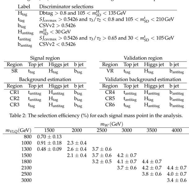
Table 1: Selection regions used in the analysis. Tagging discriminator selections and regions described in the text are explicitly defined here. The signal region (SR) is used to set cross section upper limits, the control regions (CRN) are used to estimate the QCD background, and the validation region (VR) is used to validate the background estimation procedure.

Label Discriminator selections

Htag Dbtag>0.8 and 105<mH_SD<135 GeV

ttag SJcsvmax>0.5426 and τ3/τ2 <0.8 and 105< mt_SD <210 GeV

btag CSVv2>0.5426

Hantitag mHSD<30 GeV

tantitag SJcsvmax>0.5426 and τ3/τ2 >0.65 and 30< mt_SD <105 GeV

bantitag CSVv2<0.5426

Signal region

Region Top jet Higgs jet b jet

SR ttag Htag btag

Background estimation

Region Top jet Higgs jet b jet

CR1 tantitag Hantitag btag

CR2 tantitag Htag btag

CR3 ttag Hantitag btag

Validation region

Region Top jet Higgs jet b jet

VR ttag Htag bantitag

Validation background estimation

Region Top jet Higgs jet b jet

CR4 tantitag Hantitag bantitag

CR5 tantitag Htag bantitag

CR6 ttag Hantitag bantitag

Table 2: The selection efficiency (%) for each signal mass point in the analysis. m_W0(GeV) mVLQ(GeV) 1500 2000 2500 3000 3500 4000 800 0.70_±0.13 1000 0.91±0.18 2.3±0.4 1300 0.48±0.09 2.6±0.4 3.7±0.6 1500 2.1±0.4 3.7±0.6 4.2±0.7 1800 3.2±0.5 4.1±0.7 4.4±0.7 2100 3.7±0.6 4.2±0.7 4.4±0.7 2500 3.8_±0.6 4.0_±0.7 3000 3.4_±0.6

the Higgs boson jet selection. The resulting distribution is used as the background estimate for the signal region. The primary assumption for the background estimate method is that the top jet substructure selection can be inverted without largely biasing the Higgs jet substructure selection.

A set of control regions are defined by requiring the Higgs jet candidate mH

SD to be less than

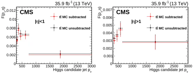
30 GeV with no double-b tagging selection. Table 1 defines various selection regions used in the analysis. A transfer function F(pT, η)is extracted from data by inverting the top jet candidate

mt_SDselection to be between 30 and 105 GeV and τ3/τ2>0.65. In this region, F(pT, η)is defined

as the ratio of the jet pT spectrum of the tagged Higgs candidate in two η regions (central,

|η| <1.0, and forward,|η| >1.0) for the full Higgs jet selection (CR2) to the inverted selection

(CR1) and is shown in Fig. 4. The F(pT, η)distribution is used to transform the normalization

and shape of distributions from the Hantitagregion to the Htagselection region, and is measured

with low signal contamination.

ac-complished by defining a control region in data with identical top and b jet candidate selections as in the signal region, but with the inverted Higgs jet selection (CR3). In this region, the mtHb

template is created using F(pT, η)as an event weight in a given Higgs candidate jet pT, η bin.

This weighted template is used as the QCD background estimate in the signal region.

In the F(pT, η)extraction procedure, the tt production component is subtracted from data in all

distributions used for creating F(pT, η)in order to ensure that F(pT, η)refers only to the QCD

component. The fraction of tt simulation subtracted from the numerator and denominator is low, 7.3 and 0.4% of the total distribution, respectively. Additionally, the tt contamination of the QCD background estimate in the signal region must to be subtracted. This is performed by applying the QCD background estimation procedure to simulated tt events using the same

F(pT, η)as is used when extracting the QCD estimate from data. The estimated contribution

accounts for 2.6% of the total QCD estimate in the signal region, which is then subtracted when forming the background estimate. The tt contamination has only a small effect on the QCD background estimation, so the systematic uncertainty due to the tt subtraction procedure is conservatively taken as the difference between the QCD background estimate extracted with and without the full tt subtraction procedure.

In order to test the applicability and versatility of the background estimate in data, a valida-tion region, VR as defined in Table 1, is defined based on inverting the b tagging criterion on the b candidate jet, with the corresponding control regions for background estimation (CR4– CR6). The transfer function in this validation region Fv(pT, η) is estimated from the ratio of

CR5 to CR4 using the same parameterization as F(pT, η). The mtHb background validation test

in this region can be seen in Fig. 5. This region validates the background estimate analog with

a χ2/ndf of 0.3 with systematic uncertainties taken into account, where ndf is the number of

degrees of freedom. The tt component in this validation region is removed using the same

procedure that is used in the signal region background estimate. The agreement in the mtHb

distribution background validation test demonstrates that the top jet selection can be inverted without biasing the Higgs jet selection. The Higgs jet candidate 4-vector mass for the SR back-ground estimate is set to the mean of the distribution extracted from the VR in order to correct

the small kinematic bias from the mass selection when forming the mtHb invariant mass. This

correction has only a small effect on the resulting distribution because of the fact that the jet

pT is large compared to the mass, and a systematic uncertainty is evaluated as the root mean

square of the distribution in the VR.

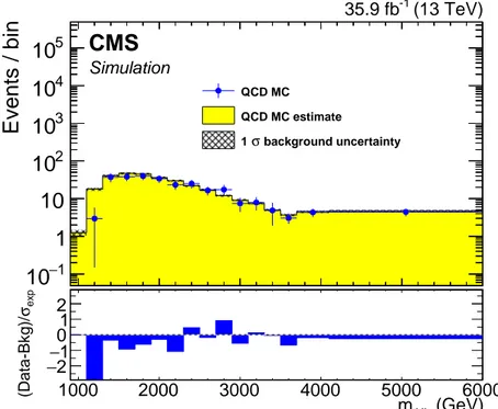
Additionally, the background validation can be studied with simulated QCD events. Figure 6 shows the level of background agreement where the SR selection and QCD background are evaluated using only simulated QCD events with the same method as was previously

described for data. A χ2/ndf of 1.4 is observed, and an additional systematic uncertainty is

included when evaluating the QCD background estimate in collision data. This correction is extracted from the ratio of the SR to QCD background in the QCD MC validation test, and is ap-plied using an interpolation of the ratio in order to decrease the effect of statistical fluctuations but to still keep the increased uncertainty at low mtHb.

The tt component is estimated by using simulation with an additional event weight to correct the generator top jet pTdistribution [45]. This generator correction is used in order to improve

the agreement of MC with data with respect to a known generator level mismodelling and is cross checked in the VR region.

T

Higgs candidate jet p

500 1000 1500 2000 2500 3000 ) η , _T F(p 0 0.002 0.004 0.006 0.008 0.01 0.012 (13 TeV) -1 35.9 fb

CMS

Higgs candidate jet p

500 1000 1500 2000 2500 3000 ) η , _T F(p 0 0.001 0.002 0.003 0.004 0.005 0.006 0.007 (13 TeV) -1 35.9 fb

CMS

Figure 4: Transfer function F(pT, η)used for estimation of the QCD background in the signal

region, shown in the central (left) and forward (right) η regions. The error bars represent the statistical uncertainty in F(pT, η)only.

6

Systematic uncertainties

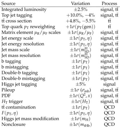
This analysis considers a wide range of systematic uncertainties that are organized into those that impact only the event yields, which are assumed to follow a log-normal distribution [46],

and those that affect the mtHb distribution shape as well. All of the systematic uncertainties

considered in the analysis are summarized in Table 3.

6.1 Normalization uncertainties

The uncertainty in the integrated luminosity is taken as 2.5% for the data set used in the analy-sis [21].

The uncertainty in the correction to the efficiency of top jet tagging algorithm is between ₋4

and+10% of the nominal value.

The theoretical uncertainty in the tt production cross section is taken into account as an

asym-metric uncertainty between −5.5 and +4.8% that is calculated as the quadrature sum of the

scale and PDF uncertainties on the overall cross section.

6.2 Shape uncertainties

The uncertainty in the jet energy scale is taken into account by scaling the four-vectors used in reconstructing the mtHbdistribution by the±1σ jet energy scale uncertainty, which is

approxi-mately 2% for jets in the analysis. The jet energy scale variation impacts the m_tHb distribution shape through a horizontal shift but can also cause a normalization difference in the case that the jet falls above or below the kinematic threshold. The uncertainty in the jet energy resolution is also taken into account by the±1σ uncertainty in the jet energy resolution correction used for simulated samples. This uncertainty is applied to all simulated samples used in the analysis, and has only a small impact.

The uncertainty in the jet mass scale and resolution is measured in a highly enriched sample of tt containing one final state lepton. In this sample, a fit is performed to the W boson jet mass

peak in the corresponding AK8 jet PUPPI mH

SDdistribution, in which the mean and width of

the PUPPI mH_SDspectrum is extracted. The mass scale uncertainty is estimated from the shift of the W mass peak to be 0.94%. The uncertainty in the mass resolution is estimated from the W

(GeV)

m

1000

2000

3000

4000

5000

6000

Events / bin

10

1

10

10

10

10

10

10

CMS

Figure 5: Reconstructed W0mass distributions (mtHb) in the b candidate inverted validation

re-gion (VR) shown for data and background contributions. Several signal hypotheses are shown to demonstrate the low signal contamination. The background uncertainty includes all system-atic and statistical uncertainties.

boson mass peak width to be 20%. These uncertainties are applied to the signal estimate used in the analysis, and result in approximately 4 and 6% variations in the overall yield for the scale and resolution uncertainties, respectively. The differences in the W and Higgs boson tagging efficiencies are estimated from a comparison of parton showering methods and are found to be between 4–5%, so an additional 5% uncertainty is included for the signal simulated samples used in the analysis.

The uncertainty used for the b tagging requirement on the AK4 jet is evaluated by varying

the b tagging and b mistagging scale factor within their ±1σ uncertainty and are considered

uncorrelated with each other. Given the kinematic selection on the AK4 jet, this uncertainty is

evaluated in four pT regions from 200–1000 GeV. For jets with a pT outside of this region, the

uncertainty is evaluated as twice the uncertainty at 1000 GeV. This uncertainty is applied to all simulated samples used in the analysis, and results in approximately a 2% effect.

The double-b tagging uncertainty used for the Higgs jet tagging [43] selection is evaluated by

varying the double-b tagging scale factor by the±1σ uncertainty. The scale factor is

parame-terized using three regions in pT. Similar to the AK4 b tagging uncertainty, outside of the

kine-matic range of the scale factor, the uncertainty is evaluated at twice the maximum range. The double-b tagging scale factor uncertainty results in approximately a 5% effect. Also evaluated is the mistag scale factor in the case of a Higgs boson mistagged as a top quark, as explained in Section 4. The uncertainties in both the Higgs jet tagging efficiency and the mistag rate are applied to all simulated samples used in the analysis, and are treated as uncorrelated with each other during limit setting.

The events used by the analysis are largely collected where the trigger efficiency is near 100%, however the small inefficiency is evaluated using the trigger efficiency extracted from data as

(GeV)

m

1000

2000

3000

4000

5000

6000

Events / bin

10

1

10

10

10

10

10

CMS

Figure 6: Reconstructed W0mass distributions (mtHb) for the simulated QCD events in the

sig-nal region for the purposes of validation. The agreement given the systematic uncertainties is at the 1 standard deviation level. The background uncertainty takes into account all systematic and statistical uncertainties.

parameterized in HT (see Fig. 2), and the uncertainty is evaluated as half of this inefficiency.

This uncertainty is small (<1%), and is applied to all simulated samples used in the analysis. As mentioned in Section 3, the simulated pileup distribution is reweighted to match data using an effective total inelastic cross section of 69.2 mb. The uncertainty in this procedure is evalu-ated by varying the total inelastic cross section by_±4.6% [47]. This uncertainty is applied to all simulated samples used in the analysis, and has only a small impact.

The mtHb distribution from the tt simulation is reweighted to correct for known differences in

the generator pTspectrum [45]. The±1σ shape uncertainty in this procedure is estimated from

the difference with the unweighted distribution. This uncertainty is applied to the tt simulated sample used in the analysis, and results in approximately a 21% effect.

The PDF uncertainty is evaluated using the NNPDF3.0 set [48]. The NNPDF set uses MC repli-cas, from which the uncertainty is evaluated as the RMS of the distribution of the associated

weights, and is then added in quadrature with the αs uncertainty. In the case of signal, the

shapes are then normalized to the nominal distribution, as to only preserve the shape of the PDF uncertainty. The normalization component of the PDF uncertainty is considered an uncer-tainty in the signal cross section.

The renormalization and factorization (µRand µF) scale uncertainty is evaluated using event

weights provided for varying the µRor µFscales up and down by a factor of two. There are

six total weights that represent the independent and simultaneous variation of µRand µF. Per

event, all weights are considered and the envelope is then used as the±1σ uncertainty band.

This uncertainty is applied to the tt MC sample used in the analysis, and results in an approx-imately 30% effect. Similar to the PDF uncertainty, the normalization component of this un-certainty is taken as the signal cross section theoretical unun-certainty, and the shape component

alone is used for limit setting.

The analysis considers five sources of uncertainty in the shape of the QCD background estimate derived from data. The statistical uncertainty in F(pT, η)is propagated to the mtHbspectrum by

evaluating the F(pT, η)weight at±1σ in a given (pT, η) bin. The uncertainty from each F(pT, η)

bin is added in quadrature to form the full uncertainty in the mtHbtemplate. The up and down

uncertainty variation in the tt subtraction procedure is taken as the unsubtracted mtHb

dis-tribution and the resulting mtHb distribution given twice the subtraction. The uncertainty in

the four vector Higgs jet candidate mass modification is taken as_±30 GeV. The “nonclosure”

uncertainty in the QCD background estimate is evaluated as the difference between the full selection and background prediction from the QCD MC closure test using the interpolated ra-tio, and is the leading source of uncertainty in the QCD background estimate of approximately 20%.

The MC statistical uncertainty is taken into account using the “Barlow–Beeston lite” method [49] during limit setting.

Table 3: Sources of systematic uncertainty affecting the m_tHb distribution. Sources that list the systematic variation as_±1σ depend on the distribution of the variable given in the parentheses, while those that list the variation in percent are rate uncertainties.

Source Variation Process

Integrated luminosity ±2.5% signal, tt

Top jet tagging +10.0%,−4% signal, tt

tt cross section +4.8%,₋5.5% tt

Top quark pTreweighting +1σ(pT(gen)) tt

Matrix element µR/µFscales ±1σ(µR/µF) signal, tt

Jet energy scale _±1σ(pT, η) signal, tt

Jet energy resolution ±1σ(pT, η) signal, tt

Jet mass scale ±1σ(mH_SD) signal, tt

Jet mass resolution _±1σ(mH_SD) signal, tt

b tagging _±1σ(pT) signal, tt

b mistagging _±1σ(pT) signal, tt

Double-b tagging ±1σ(pT) signal, tt

Double-b mistagging ±1σ(pT) signal, tt

Higgs jet tagging ±5% signal

Pileup ±1σ (σmb) signal, tt

PDF _±1σ(Q2, x) signal, tt

HTtrigger ±1σ(HT) signal, tt

tt contamination _±1σ(pT) QCD

F(pT, η) ±1σ(pT, η) QCD

Higgs jet mass modification ±1σ(mH) QCD

Nonclosure ±1σ(mtHb) QCD

7

Results

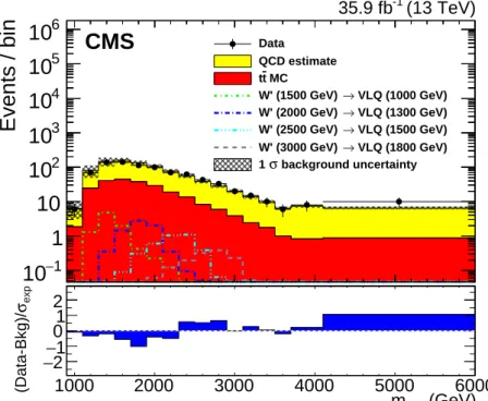
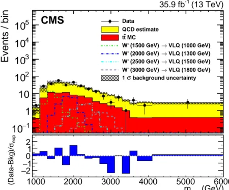
The final mtHbdistribution is shown in Fig. 7, with a χ2/ndf of 1.3 for the agreement of data and

background. Table 4 shows the yield for data, QCD and tt backgrounds, for various selection regions including the full selection.

Using a Bayesian approach with a flat prior for the signal cross section, upper limits are ob-tained on the product of the W0boson production cross section in the sL =0.5 and cot(θ2) =3

(GeV)

m

1000

2000

3000

4000

5000

6000

Events / bin

10

1

10

10

10

10

10

CMS

Figure 7: Reconstructed W0 mass distributions (mtHb) in the signal region, compared with the

distributions of estimated backgrounds, and several benchmarks models. The signal

distribu-tions include the contribudistribu-tions from W0 decays to both the T and B assuming equal branching

fractions. The uncertainties shown in the hatched region contain both statistical and systematic uncertainties of all background components.

Table 4: Event yield table after various selections. The definition of each region is given in Table 1. The uncertainties shown here for the validation region and the signal region are pre fit; the posteriori uncertainties for tt and QCD are constrained down by 40 and 14%, respectively.

Region Data QCD tt CR1 79 104 — 332 CR2 398 — 25 CR3 45 646 — 1365 CR4 288 926 — 543 CR5 1 330 — 76 CR6 154 608 — 1991 VR 844±30 659±150 236±83 SR 284±17 208±49 71±28

hypothesis, and the benchmark W0 _→ T/B _→ tHb branching fraction. A binned likelihood

is used to calculate 95% confidence level (CL) upper limits, in a process where all systematic uncertainties listed in Section 6 that affect the shape of the mtHb distribution are included as

nuisance parameters that modify the shape using template interpolation, and those that affect the normalization are included as nuisance parameters with lognormal priors. For the signal

template, the sum of reconstructed mtHbdistribution from the tB and bT decay channels is used.

Pseudo-experiments are used to derive the_±1σ deviations in the expected limit. The

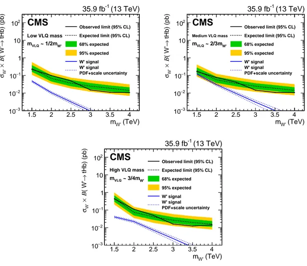
system-atic uncertainties described above are accounted for as nuisance parameters and the posterior probability is refitted for each pseudo-experiment. Cross section upper limits are shown in

at a value of 0.85 standard deviations. Although no signal mass points are excluded by solely

analyzing the all hadronic W0 _→T/B_→tHb decay in the democratic bT and tB decay

hypoth-esis, a W0with a mass below 1.6 TeV is excluded at 95% CL in the case of a 100% bT branching

fraction hypothesis. (TeV) W' m 1.5 2 2.5 3 3.5 4 tHb) (pb) → ( W' Β × W' σ 3 − 10 2 − 10 1 − 10 1 10 2 10 (13 TeV) -1 35.9 fb

CMS

CMS

CMS

Figure 8: The W0 boson 95% CL production cross section limits. The expected limits (dashed)

and observed limits (solid), as well as the W0 boson theoretical cross section and the PDF and

scale normalization uncertainties are shown. The bands around the expected limit represent the

±1 and±2σexp uncertainties in the expected limit. The limits for low- (upper left),

medium-(upper right), and high- (lower) mass VLQ mass ranges, defined in Table 2, are shown.

8

Summary

A search for a heavy W0 boson decaying to a B or T vector-like quark and a top or b quark,

respectively, has been presented. The data correspond to an integrated luminosity of 35.9 fb−1

collected in 2016 with the CMS detector at the LHC. The signature considered for both decay modes is a top quark and a Higgs boson, both decaying hadronically, and a b quark jet. Boosted heavy-resonance identification techniques are used to exploit the event signature of three en-ergetic jets and to suppress standard model backgrounds. No significant deviation from the

standard model background prediction has been observed. Cross section upper limits on W0

boson production in the top quark, Higgs boson, and b quark decay mode are set as a function of the W0 mass, for several vector-like quark mass hypotheses. These are the first limits for W0

boson production in this decay channel, and cover a range of 0.01 to 0.43 pb in the W0 mass range between 1.5 and 4.0 TeV.

Acknowledgments

We congratulate our colleagues in the CERN accelerator departments for the excellent perfor-mance of the LHC and thank the technical and administrative staffs at CERN and at other CMS institutes for their contributions to the success of the CMS effort. In addition, we gratefully acknowledge the computing centers and personnel of the Worldwide LHC Computing Grid for delivering so effectively the computing infrastructure essential to our analyses. Finally, we acknowledge the enduring support for the construction and operation of the LHC and the CMS detector provided by the following funding agencies: BMBWF and FWF (Austria); FNRS and FWO (Belgium); CNPq, CAPES, FAPERJ, FAPERGS, and FAPESP (Brazil); MES (Bulgaria); CERN; CAS, MoST, and NSFC (China); COLCIENCIAS (Colombia); MSES and CSF (Croa-tia); RPF (Cyprus); SENESCYT (Ecuador); MoER, ERC IUT, and ERDF (Estonia); Academy of Finland, MEC, and HIP (Finland); CEA and CNRS/IN2P3 (France); BMBF, DFG, and HGF (Germany); GSRT (Greece); NKFIA (Hungary); DAE and DST (India); IPM (Iran); SFI (Ireland); INFN (Italy); MSIP and NRF (Republic of Korea); MES (Latvia); LAS (Lithuania); MOE and UM (Malaysia); BUAP, CINVESTAV, CONACYT, LNS, SEP, and UASLP-FAI (Mexico); MOS (Mon-tenegro); MBIE (New Zealand); PAEC (Pakistan); MSHE and NSC (Poland); FCT (Portugal); JINR (Dubna); MON, RosAtom, RAS, RFBR, and NRC KI (Russia); MESTD (Serbia); SEIDI, CPAN, PCTI, and FEDER (Spain); MOSTR (Sri Lanka); Swiss Funding Agencies (Switzerland); MST (Taipei); ThEPCenter, IPST, STAR, and NSTDA (Thailand); TUBITAK and TAEK (Turkey); NASU and SFFR (Ukraine); STFC (United Kingdom); DOE and NSF (USA).

Individuals have received support from the Marie-Curie program and the European Research Council and Horizon 2020 Grant, contract No. 675440 (European Union); the Leventis Foun-dation; the A. P. Sloan FounFoun-dation; the Alexander von Humboldt FounFoun-dation; the Belgian Federal Science Policy Office; the Fonds pour la Formation `a la Recherche dans l’Industrie et dans l’Agriculture (FRIA-Belgium); the Agentschap voor Innovatie door Wetenschap en Tech-nologie (IWT-Belgium); the F.R.S.-FNRS and FWO (Belgium) under the “Excellence of Science - EOS” - be.h project n. 30820817; the Ministry of Education, Youth and Sports (MEYS) of the Czech Republic; the Lend ¨ulet (“Momentum”) Programme and the J´anos Bolyai Research Scholarship of the Hungarian Academy of Sciences, the New National Excellence Program

´

UNKP, the NKFIA research grants 123842, 123959, 124845, 124850 and 125105 (Hungary); the Council of Science and Industrial Research, India; the HOMING PLUS program of the Foun-dation for Polish Science, cofinanced from European Union, Regional Development Fund, the Mobility Plus program of the Ministry of Science and Higher Education, the National Science Center (Poland), contracts Harmonia 2014/14/M/ST2/00428, Opus 2014/13/B/ST2/02543, 2014/15/B/ST2/03998, and 2015/19/B/ST2/02861, Sonata-bis 2012/07/E/ST2/01406; the National Priorities Research Program by Qatar National Research Fund; the Programa Estatal de Fomento de la Investigaci ´on Cient´ıfica y T´ecnica de Excelencia Mar´ıa de Maeztu, grant MDM-2015-0509 and the Programa Severo Ochoa del Principado de Asturias; the Thalis and Aristeia program cofinanced by EU-ESF and the Greek NSRF; the Rachadapisek Sompot Fund for Postdoctoral Fellowship, Chulalongkorn University and the Chulalongkorn Academic into Its 2nd Century Project Advancement Project (Thailand); the Welch Foundation, contract C-1845; and the Weston Havens Foundation (USA).

References

[1] M. Schmaltz and D. Tucker-Smith, “Little Higgs theories”, Ann. Rev. of Nucl. and Part. Sci.

55(2005) 229, doi:10.1146/annurev.nucl.55.090704.151502,

arXiv:hep-ph/0502182.

[2] T. Appelquist, H.-C. Cheng, and B. A. Dobrescu, “Bounds on universal extra

dimensions”, Phys. Rev. D 64 (2001) 035002, doi:10.1103/PhysRevD.64.035002,

arXiv:hep-ph/0012100.

[3] R. N. Mohapatra and J. C. Pati, “Left-right gauge symmetry and an ’isoconjugate’ model of CP violation”, Phys. Rev. D 11 (1975) 566, doi:10.1103/PhysRevD.11.566.

[4] CMS Collaboration, “Search for heavy gauge W’ boson in events with an energetic lepton

and large missing transverse momentum at√s=13 TeV”, Phys. Lett. B 770 (2017)

doi:10.1016/j.physletb.2017.04.043, arXiv:1612.09274.

[5] ATLAS Collaboration, “Search for a new heavy gauge boson resonance decaying into a

lepton and missing transverse momentum in 36 fb−1of pp collisions at√s=13 TeV with

the ATLAS experiment”, Eur. Phys. J. C 78 (2018) 401,

doi:10.1140/epjc/s10052-018-5877-y, arXiv:1706.04786.

[6] CMS Collaboration, “Search for a heavy resonance decaying to a pair of vector bosons in

the lepton plus merged jet final state at√s =13 TeV”, JHEP 05 (2018) 088,

doi:10.1007/JHEP05(2018)088, arXiv:1802.09407.

[7] ATLAS Collaboration, “Search for WW/WZ resonance production in νqq final states in

pp collisions at√s=13 TeV with the ATLAS detector”, JHEP 03 (2018) 042,

doi:10.1007/JHEP03(2018)042, arXiv:1710.07235.

[8] CMS Collaboration, “Searches for W0bosons decaying to a top quark and a bottom quark

in proton-proton collisions at 13 TeV”, JHEP 08 (2017) 029,

doi:10.1007/JHEP08(2017)029, arXiv:1706.04260.

[9] ATLAS Collaboration, “Search for W0 _→tb decays in the hadronic final state using pp

collisions at√s=13 TeV with the ATLAS detector”, Phys. Lett. B 781 (2018) 327,

doi:10.1016/j.physletb.2018.03.036, arXiv:1801.07893.

[10] CMS Collaboration, “Search for single production of a vector-like T quark decaying to a

Z boson and a top quark in proton-proton collisions at√s = 13 TeV”, Phys. Lett. B 781

(2018) 574, doi:10.1016/j.physletb.2018.04.036, arXiv:1708.01062. [11] CMS Collaboration, “Search for single production of vector-like quarks decaying to a b

quark and a Higgs boson”, JHEP 06 (2018) 031, doi:10.1007/JHEP06(2018)031,

arXiv:1802.01486.

[12] ATLAS Collaboration, “Search for pair- and single-production of vector-like quarks in final states with at least one Z boson decaying into a pair of electrons or muons in pp

collision data collected with the ATLAS detector at√s=13 TeV”, (2018).

arXiv:1806.10555.

[13] CMS Collaboration, “Search for single production of vector-like quarks decaying into a b

quark and a W boson in proton-proton collisions at√s=13 TeV”, Phys. Lett. B 772

[14] CMS Collaboration, “Search for pair production of vector-like quarks in the bWbW

channel from proton-proton collisions at√s = 13 TeV”, Phys. Lett. B 779 (2018) 82,

doi:10.1016/j.physletb.2018.01.077, arXiv:1710.01539.

[15] CMS Collaboration, “Search for vector-like T and B quark pairs in final states with

leptons at√s=13 TeV”, (2018). arXiv:1805.04758.

[16] ATLAS Collaboration, “Combination of the searches for pair-produced vector-like

partners of the third-generation quarks at√s =13 TeV with the ATLAS detector”, (2018).

arXiv:1808.02343.

[17] K. Agashe, R. Contino, and A. Pomarol, “The minimal composite Higgs model”, Nucl. Phys. B 719 (2005) 165, doi:10.1016/j.nuclphysb.2005.04.035,

arXiv:hep-ph/0412089.

[18] D. Barducci et al., “Exploring drell-yan signals from the 4d composite higgs model at the lhc”, JHEP 04 (2013) 152, doi:10.1007/JHEP04(2013)152, arXiv:1210.2927. [19] D. Barducci and C. Delaunay, “Bounding wide composite vector resonances at the lhc”,

JHEP 02 (2016) 55, doi:10.1007/JHEP02(2016)055, arXiv:1511.01101.

[20] N. Vignaroli, “New W0 signals at the LHC”, Phys. Rev. D 89 (2014) 095027,

doi:10.1103/PhysRevD.89.095027, arXiv:1404.5558.

[21] CMS Collaboration, “CMS luminosity measurements for the 2016 data taking period”, CMS Physics Analysis Summary CMS-PAS-LUM-17-001, CERN, Geneva, 2017.

[22] CMS Collaboration, “The CMS experiment at the CERN LHC”, JINST 3 (2008) S08004, doi:10.1088/1748-0221/3/08/S08004.

[23] CMS Collaboration, “Particle-flow reconstruction and global event description with the CMS detector”, JINST 12 (2017) P10003, doi:10.1088/1748-0221/12/10/P10003,

arXiv:1706.04965.

[24] M. Cacciari, G. P. Salam, and G. Soyez, “The anti-kTjet clustering algorithm”, JHEP 04

(2008) 063, doi:10.1088/1126-6708/2008/04/063, arXiv:0802.1189.

[25] M. Cacciari, G. P. Salam, and G. Soyez, “Fastjet user manual”, Eur. Phys. J. C 72 (2012) 1896, doi:10.1140/epjc/s10052-012-1896-2, arXiv:1111.6097.

[26] D. Bertolini, P. Harris, M. Low, and N. Tran, “Pileup per particle identification”, JHEP 10 (2014) 059, doi:10.1007/JHEP10(2014)059, arXiv:1407.6013.

[27] CMS Collaboration, “Jet energy scale and resolution in the CMS experiment in pp collisions at 8 TeV”, JINST 12 (2017) P02014,

doi:10.1088/1748-0221/12/02/P02014, arXiv:1607.03663.

[28] CMS Collaboration, “The CMS trigger system”, JINST 12 (2017) P01020, doi:10.1088/1748-0221/12/01/P01020, arXiv:1609.02366.

[29] S. Frixione, P. Nason, and C. Oleari, “Matching NLO QCD computations with parton shower simulations: the POWHEG method”, JHEP 11 (2007) 070,

[30] S. Alioli, P. Nason, C. Oleari, and E. Re, “A general framework for implementing NLO calculations in shower Monte Carlo programs: the POWHEG BOX”, JHEP 06 (2010) 043, doi:10.1007/JHEP06(2010)043, arXiv:1002.2581.

[31] P. Nason, “A new method for combining NLO QCD with shower Monte Carlo algorithms”, JHEP 11 (2004) 040, doi:10.1088/1126-6708/2004/11/040, arXiv:hep-ph/0409146.

[32] S. Frixione, P. Nason, and G. Ridolfi, “A positive-weight next-to-leading-order Monte Carlo for heavy flavour hadroproduction”, JHEP 09 (2007) 126,

doi:10.1088/1126-6708/2007/09/126, arXiv:0707.3088.

[33] J. Alwall et al., “The automated computation of tree-level and next-to-leading order differential cross sections, and their matching to parton shower simulations”, JHEP 07 (2014) 079, doi:10.1007/JHEP07(2014)079, arXiv:1405.0301.

[34] J. Alwall et al., “Comparative study of various algorithms for the merging of parton showers and matrix elements in hadronic collisions”, Eur. Phys. J. C 53 (2008) 473,

doi:10.1140/epjc/s10052-007-0490-5, arXiv:0706.2569.

[35] T. Sj ¨ostrand et al., “An introduction to PYTHIA 8.2”, Comput. Phys. Commun. 191 (2015) 159, doi:10.1016/j.cpc.2015.01.024, arXiv:1410.3012.

[36] CMS Collaboration, “Investigations of the impact of the parton shower tuning in Pythia 8

in the modelling of tt at√s =8 and 13 TeV”, Technical Report CMS-PAS-TOP-16-021,

CERN, Geneva, 2016.

[37] CMS Collaboration, “Event generator tunes obtained from underlying event and multiparton scattering measurements”, Eur. Phys. J. C 76 (2016) 155,

doi:10.1140/epjc/s10052-016-3988-x, arXiv:1512.00815.

[38] GEANT4 Collaboration, “GEANT4—a a simulation toolkit”, Nucl. Instrum. Meth. 506

(2003) 250, doi:10.1016/S0168-9002(03)01368-8.

[39] CMS Collaboration, “Jet algorithms performance in 13 TeV data”, CMS Physics Analysis Summary CMS-PAS-JME-16-003, CERN, Geneva, 2017.

[40] J. Thaler and K. Van Tilburg, “Maximizing boosted top identification by minimizing N-subjettiness”, JHEP 02 (2012) 093, doi:10.1007/JHEP02(2012)093,

arXiv:1108.2701.

[41] M. Dasgupta, A. Fregoso, S. Marzani, and G. P. Salam, “Towards an understanding of jet substructure”, JHEP 09 (2013) 029, doi:10.1007/JHEP09(2013)029,

arXiv:1307.0007.

[42] A. J. Larkoski, S. Marzani, G. Soyez, and J. Thaler, “Soft drop”, JHEP 05 (2014)

doi:10.1007/JHEP05(2014)146, arXiv:1402.2657.

[43] CMS Collaboration, “Identification of heavy-flavour jets with the CMS detector in pp collisions at 13 TeV”, JINST 13 (2018) P05011,

doi:10.1088/1748-0221/13/05/P05011, arXiv:1712.07158.

[44] CMS Collaboration, “Search for massive resonances decaying into WW, WZ, ZZ, qW,

and qZ with dijet final states at√s=13 TeV”, Phys. Rev. D 97 (2018) 072006,

[45] CMS Collaboration, “Measurement of differential cross sections for top quark pair production using the lepton+jets final state in proton-proton collisions at 13 TeV”, Phys. Rev. D 95 (2017) 092001, doi:10.1103/PhysRevD.95.092001, arXiv:1610.04191. [46] J. S. Conway, “Incorporating nuisance parameters in likelihoods for multisource spectra”,

in Proceedings, PHYSTAT 2011 workshop on statistical issues related to discovery claims in search experiments and unfolding, CERN,Geneva, Switzerland 17-20 January 2011, p. 115. 2011. arXiv:1103.0354. doi:10.5170/CERN-2011-006.115.

[47] CMS Collaboration, “Measurement of the inelastic proton-proton cross section at√s=13

TeV”, JHEP 07 (2018) 161, doi:10.1007/JHEP07(2018)161, arXiv:1802.02613. [48] NNPDF Collaboration, “Parton distributions from high-precision collider data”, Eur.

Phys. J. C 77 (2017) 663, doi:10.1140/epjc/s10052-017-5199-5,

arXiv:1706.00428.

[49] R. Barlow and C. Beeston, “Fitting using finite Monte Carlo samples”, Comput. Phys. Commun. 77 (1993) 219, doi:10.1016/0010-4655(93)90005-W.

A

The CMS Collaboration

Yerevan Physics Institute, Yerevan, Armenia

A.M. Sirunyan, A. Tumasyan

Institut f ¨ur Hochenergiephysik, Wien, Austria

W. Adam, F. Ambrogi, E. Asilar, T. Bergauer, J. Brandstetter, M. Dragicevic, J. Er ¨o, A. Escalante Del Valle, M. Flechl, R. Fr ¨uhwirth1, V.M. Ghete, J. Hrubec, M. Jeitler1, N. Krammer, I. Kr¨atschmer, D. Liko, T. Madlener, I. Mikulec, N. Rad, H. Rohringer, J. Schieck1_{, R. Sch ¨ofbeck,}

M. Spanring, D. Spitzbart, A. Taurok, W. Waltenberger, J. Wittmann, C.-E. Wulz1, M. Zarucki

Institute for Nuclear Problems, Minsk, Belarus

V. Chekhovsky, V. Mossolov, J. Suarez Gonzalez

Universiteit Antwerpen, Antwerpen, Belgium

E.A. De Wolf, D. Di Croce, X. Janssen, J. Lauwers, M. Pieters, H. Van Haevermaet, P. Van Mechelen, N. Van Remortel

Vrije Universiteit Brussel, Brussel, Belgium

S. Abu Zeid, F. Blekman, J. D’Hondt, J. De Clercq, K. Deroover, G. Flouris, D. Lontkovskyi, S. Lowette, I. Marchesini, S. Moortgat, L. Moreels, Q. Python, K. Skovpen, S. Tavernier, W. Van Doninck, P. Van Mulders, I. Van Parijs

Universit´e Libre de Bruxelles, Bruxelles, Belgium

D. Beghin, B. Bilin, H. Brun, B. Clerbaux, G. De Lentdecker, H. Delannoy, B. Dorney, G. Fasanella, L. Favart, R. Goldouzian, A. Grebenyuk, A.K. Kalsi, T. Lenzi, J. Luetic, N. Postiau, E. Starling, L. Thomas, C. Vander Velde, P. Vanlaer, D. Vannerom, Q. Wang

Ghent University, Ghent, Belgium

T. Cornelis, D. Dobur, A. Fagot, M. Gul, I. Khvastunov2, D. Poyraz, C. Roskas, D. Trocino,

M. Tytgat, W. Verbeke, B. Vermassen, M. Vit, N. Zaganidis

Universit´e Catholique de Louvain, Louvain-la-Neuve, Belgium

H. Bakhshiansohi, O. Bondu, S. Brochet, G. Bruno, C. Caputo, P. David, C. Delaere, M. Delcourt, A. Giammanco, G. Krintiras, V. Lemaitre, A. Magitteri, K. Piotrzkowski, A. Saggio, M. Vidal Marono, P. Vischia, S. Wertz, J. Zobec

Centro Brasileiro de Pesquisas Fisicas, Rio de Janeiro, Brazil

F.L. Alves, G.A. Alves, M. Correa Martins Junior, G. Correia Silva, C. Hensel, A. Moraes, M.E. Pol, P. Rebello Teles

Universidade do Estado do Rio de Janeiro, Rio de Janeiro, Brazil

E. Belchior Batista Das Chagas, W. Carvalho, J. Chinellato3, E. Coelho, E.M. Da Costa,

G.G. Da Silveira4, D. De Jesus Damiao, C. De Oliveira Martins, S. Fonseca De Souza,

H. Malbouisson, D. Matos Figueiredo, M. Melo De Almeida, C. Mora Herrera, L. Mundim, H. Nogima, W.L. Prado Da Silva, L.J. Sanchez Rosas, A. Santoro, A. Sznajder, M. Thiel, E.J. Tonelli Manganote3_{, F. Torres Da Silva De Araujo, A. Vilela Pereira}

Universidade Estadual Paulistaa, Universidade Federal do ABCb, S˜ao Paulo, Brazil

S. Ahujaa, C.A. Bernardesa, L. Calligarisa, T.R. Fernandez Perez Tomeia, E.M. Gregoresb, P.G. Mercadanteb, S.F. Novaesa, SandraS. Padulaa

Bulgaria

A. Aleksandrov, R. Hadjiiska, P. Iaydjiev, A. Marinov, M. Misheva, M. Rodozov, M. Shopova, G. Sultanov

University of Sofia, Sofia, Bulgaria

A. Dimitrov, L. Litov, B. Pavlov, P. Petkov

Beihang University, Beijing, China

W. Fang5, X. Gao5, L. Yuan

Institute of High Energy Physics, Beijing, China

M. Ahmad, J.G. Bian, G.M. Chen, H.S. Chen, M. Chen, Y. Chen, C.H. Jiang, D. Leggat, H. Liao, Z. Liu, S.M. Shaheen6, A. Spiezia, J. Tao, Z. Wang, E. Yazgan, H. Zhang, S. Zhang6, J. Zhao

State Key Laboratory of Nuclear Physics and Technology, Peking University, Beijing, China

Y. Ban, G. Chen, A. Levin, J. Li, L. Li, Q. Li, Y. Mao, S.J. Qian, D. Wang

Tsinghua University, Beijing, China

Y. Wang

Universidad de Los Andes, Bogota, Colombia

C. Avila, A. Cabrera, C.A. Carrillo Montoya, L.F. Chaparro Sierra, C. Florez,

C.F. Gonz´alez Hern´andez, M.A. Segura Delgado

University of Split, Faculty of Electrical Engineering, Mechanical Engineering and Naval Architecture, Split, Croatia

B. Courbon, N. Godinovic, D. Lelas, I. Puljak, T. Sculac

University of Split, Faculty of Science, Split, Croatia

Z. Antunovic, M. Kovac

Institute Rudjer Boskovic, Zagreb, Croatia

V. Brigljevic, D. Ferencek, K. Kadija, B. Mesic, A. Starodumov7, T. Susa

University of Cyprus, Nicosia, Cyprus

M.W. Ather, A. Attikis, M. Kolosova, G. Mavromanolakis, J. Mousa, C. Nicolaou, F. Ptochos, P.A. Razis, H. Rykaczewski

Charles University, Prague, Czech Republic

M. Finger8, M. Finger Jr.8

Escuela Politecnica Nacional, Quito, Ecuador

E. Ayala

Universidad San Francisco de Quito, Quito, Ecuador

E. Carrera Jarrin

Academy of Scientific Research and Technology of the Arab Republic of Egypt, Egyptian Network of High Energy Physics, Cairo, Egypt

M.A. Mahmoud9,10, Y. Mohammed9, E. Salama10,11

National Institute of Chemical Physics and Biophysics, Tallinn, Estonia

S. Bhowmik, A. Carvalho Antunes De Oliveira, R.K. Dewanjee, K. Ehataht, M. Kadastik, M. Raidal, C. Veelken

Department of Physics, University of Helsinki, Helsinki, Finland

Helsinki Institute of Physics, Helsinki, Finland

J. Havukainen, J.K. Heikkil¨a, T. J¨arvinen, V. Karim¨aki, R. Kinnunen, T. Lamp´en, K. Lassila-Perini, S. Laurila, S. Lehti, T. Lind´en, P. Luukka, T. M¨aenp¨a¨a, H. Siikonen, E. Tuominen, J. Tuominiemi

Lappeenranta University of Technology, Lappeenranta, Finland

T. Tuuva

IRFU, CEA, Universit´e Paris-Saclay, Gif-sur-Yvette, France

M. Besancon, F. Couderc, M. Dejardin, D. Denegri, J.L. Faure, F. Ferri, S. Ganjour, A. Givernaud, P. Gras, G. Hamel de Monchenault, P. Jarry, C. Leloup, E. Locci, J. Malcles, G. Negro, J. Rander, A. Rosowsky, M. ¨O. Sahin, M. Titov

Laboratoire Leprince-Ringuet, Ecole polytechnique, CNRS/IN2P3, Universit´e Paris-Saclay, Palaiseau, France

A. Abdulsalam12, C. Amendola, I. Antropov, F. Beaudette, P. Busson, C. Charlot,

R. Granier de Cassagnac, I. Kucher, A. Lobanov, J. Martin Blanco, C. Martin Perez, M. Nguyen, C. Ochando, G. Ortona, P. Paganini, P. Pigard, J. Rembser, R. Salerno, J.B. Sauvan, Y. Sirois, A.G. Stahl Leiton, A. Zabi, A. Zghiche

Universit´e de Strasbourg, CNRS, IPHC UMR 7178, Strasbourg, France

J.-L. Agram13, J. Andrea, D. Bloch, J.-M. Brom, E.C. Chabert, V. Cherepanov, C. Collard,

E. Conte13, J.-C. Fontaine13, D. Gel´e, U. Goerlach, M. Jansov´a, A.-C. Le Bihan, N. Tonon,

P. Van Hove

Centre de Calcul de l’Institut National de Physique Nucleaire et de Physique des Particules, CNRS/IN2P3, Villeurbanne, France

S. Gadrat

Universit´e de Lyon, Universit´e Claude Bernard Lyon 1, CNRS-IN2P3, Institut de Physique Nucl´eaire de Lyon, Villeurbanne, France

S. Beauceron, C. Bernet, G. Boudoul, N. Chanon, R. Chierici, D. Contardo, P. Depasse, H. El Mamouni, J. Fay, L. Finco, S. Gascon, M. Gouzevitch, G. Grenier, B. Ille, F. Lagarde,

I.B. Laktineh, H. Lattaud, M. Lethuillier, L. Mirabito, S. Perries, A. Popov14, V. Sordini,

G. Touquet, M. Vander Donckt, S. Viret

Georgian Technical University, Tbilisi, Georgia

T. Toriashvili15

Tbilisi State University, Tbilisi, Georgia

Z. Tsamalaidze8

RWTH Aachen University, I. Physikalisches Institut, Aachen, Germany

C. Autermann, L. Feld, M.K. Kiesel, K. Klein, M. Lipinski, M. Preuten, M.P. Rauch, C. Schomakers, J. Schulz, M. Teroerde, B. Wittmer

RWTH Aachen University, III. Physikalisches Institut A, Aachen, Germany

A. Albert, D. Duchardt, M. Erdmann, S. Erdweg, T. Esch, R. Fischer, S. Ghosh, A. G ¨uth, T. Hebbeker, C. Heidemann, K. Hoepfner, H. Keller, L. Mastrolorenzo, M. Merschmeyer, A. Meyer, P. Millet, S. Mukherjee, T. Pook, M. Radziej, H. Reithler, M. Rieger, A. Schmidt, D. Teyssier, S. Th ¨uer

RWTH Aachen University, III. Physikalisches Institut B, Aachen, Germany

G. Fl ¨ugge, O. Hlushchenko, T. Kress, T. M ¨uller, A. Nehrkorn, A. Nowack, C. Pistone, O. Pooth, D. Roy, H. Sert, A. Stahl16

Deutsches Elektronen-Synchrotron, Hamburg, Germany

M. Aldaya Martin, T. Arndt, C. Asawatangtrakuldee, I. Babounikau, K. Beernaert, O. Behnke,

U. Behrens, A. Berm ´udez Mart´ınez, D. Bertsche, A.A. Bin Anuar, K. Borras17, V. Botta,

A. Campbell, P. Connor, C. Contreras-Campana, V. Danilov, A. De Wit, M.M. Defranchis, C. Diez Pardos, D. Dom´ınguez Damiani, G. Eckerlin, T. Eichhorn, A. Elwood, E. Eren,

E. Gallo18, A. Geiser, J.M. Grados Luyando, A. Grohsjean, M. Guthoff, M. Haranko, A. Harb,

H. Jung, M. Kasemann, J. Keaveney, C. Kleinwort, J. Knolle, D. Kr ¨ucker, W. Lange, A. Lelek,

T. Lenz, J. Leonard, K. Lipka, W. Lohmann19, R. Mankel, I.-A. Melzer-Pellmann, A.B. Meyer,

M. Meyer, M. Missiroli, J. Mnich, V. Myronenko, S.K. Pflitsch, D. Pitzl, A. Raspereza, P. Saxena, P. Sch ¨utze, C. Schwanenberger, R. Shevchenko, A. Singh, H. Tholen, O. Turkot, A. Vagnerini, G.P. Van Onsem, R. Walsh, Y. Wen, K. Wichmann, C. Wissing, O. Zenaiev

University of Hamburg, Hamburg, Germany

R. Aggleton, S. Bein, L. Benato, A. Benecke, V. Blobel, T. Dreyer, A. Ebrahimi, E. Garutti, D. Gonzalez, P. Gunnellini, J. Haller, A. Hinzmann, A. Karavdina, G. Kasieczka, R. Klanner, R. Kogler, N. Kovalchuk, S. Kurz, V. Kutzner, J. Lange, D. Marconi, J. Multhaup, M. Niedziela, C.E.N. Niemeyer, D. Nowatschin, A. Perieanu, A. Reimers, O. Rieger, C. Scharf, P. Schleper, S. Schumann, J. Schwandt, J. Sonneveld, H. Stadie, G. Steinbr ¨uck, F.M. Stober, M. St ¨over, A. Vanhoefer, B. Vormwald, I. Zoi

Karlsruher Institut fuer Technologie, Karlsruhe, Germany

M. Akbiyik, C. Barth, M. Baselga, S. Baur, E. Butz, R. Caspart, T. Chwalek, F. Colombo, W. De Boer, A. Dierlamm, K. El Morabit, N. Faltermann, B. Freund, M. Giffels,

M.A. Harrendorf, F. Hartmann16, S.M. Heindl, U. Husemann, I. Katkov14, S. Kudella, S. Mitra,

M.U. Mozer, Th. M ¨uller, M. Musich, M. Plagge, G. Quast, K. Rabbertz, M. Schr ¨oder, I. Shvetsov, H.J. Simonis, R. Ulrich, S. Wayand, M. Weber, T. Weiler, C. W ¨ohrmann, R. Wolf

Institute of Nuclear and Particle Physics (INPP), NCSR Demokritos, Aghia Paraskevi, Greece

G. Anagnostou, G. Daskalakis, T. Geralis, A. Kyriakis, D. Loukas, G. Paspalaki

National and Kapodistrian University of Athens, Athens, Greece

A. Agapitos, G. Karathanasis, P. Kontaxakis, A. Panagiotou, I. Papavergou, N. Saoulidou, E. Tziaferi, K. Vellidis

National Technical University of Athens, Athens, Greece

K. Kousouris, I. Papakrivopoulos, G. Tsipolitis

University of Io´annina, Io´annina, Greece

I. Evangelou, C. Foudas, P. Gianneios, P. Katsoulis, P. Kokkas, S. Mallios, N. Manthos, I. Papadopoulos, E. Paradas, J. Strologas, F.A. Triantis, D. Tsitsonis

MTA-ELTE Lend ¨ulet CMS Particle and Nuclear Physics Group, E ¨otv ¨os Lor´and University, Budapest, Hungary

M. Bart ´ok20, M. Csanad, N. Filipovic, P. Major, M.I. Nagy, G. Pasztor, O. Sur´anyi, G.I. Veres

Wigner Research Centre for Physics, Budapest, Hungary

G. Bencze, C. Hajdu, D. Horvath21, ´A. Hunyadi, F. Sikler, T. ´A. V´ami, V. Veszpremi,

G. Vesztergombi†

Institute of Nuclear Research ATOMKI, Debrecen, Hungary

Institute of Physics, University of Debrecen, Debrecen, Hungary

P. Raics, Z.L. Trocsanyi, B. Ujvari

Indian Institute of Science (IISc), Bangalore, India

S. Choudhury, J.R. Komaragiri, P.C. Tiwari

National Institute of Science Education and Research, HBNI, Bhubaneswar, India

S. Bahinipati23, C. Kar, P. Mal, K. Mandal, A. Nayak24, D.K. Sahoo23, S.K. Swain

Panjab University, Chandigarh, India

S. Bansal, S.B. Beri, V. Bhatnagar, S. Chauhan, R. Chawla, N. Dhingra, R. Gupta, A. Kaur, M. Kaur, S. Kaur, P. Kumari, M. Lohan, A. Mehta, K. Sandeep, S. Sharma, J.B. Singh, A.K. Virdi, G. Walia

University of Delhi, Delhi, India

A. Bhardwaj, B.C. Choudhary, R.B. Garg, M. Gola, S. Keshri, Ashok Kumar, S. Malhotra, M. Naimuddin, P. Priyanka, K. Ranjan, Aashaq Shah, R. Sharma

Saha Institute of Nuclear Physics, HBNI, Kolkata, India

R. Bhardwaj25, M. Bharti25, R. Bhattacharya, S. Bhattacharya, U. Bhawandeep25, D. Bhowmik,

S. Dey, S. Dutt25, S. Dutta, S. Ghosh, K. Mondal, S. Nandan, A. Purohit, P.K. Rout, A. Roy,

S. Roy Chowdhury, G. Saha, S. Sarkar, M. Sharan, B. Singh25, S. Thakur25

Indian Institute of Technology Madras, Madras, India

P.K. Behera

Bhabha Atomic Research Centre, Mumbai, India

R. Chudasama, D. Dutta, V. Jha, V. Kumar, D.K. Mishra, P.K. Netrakanti, L.M. Pant, P. Shukla

Tata Institute of Fundamental Research-A, Mumbai, India

T. Aziz, M.A. Bhat, S. Dugad, G.B. Mohanty, N. Sur, B. Sutar, RavindraKumar Verma

Tata Institute of Fundamental Research-B, Mumbai, India

S. Banerjee, S. Bhattacharya, S. Chatterjee, P. Das, M. Guchait, Sa. Jain, S. Karmakar, S. Kumar,

M. Maity26, G. Majumder, K. Mazumdar, N. Sahoo, T. Sarkar26

Indian Institute of Science Education and Research (IISER), Pune, India

S. Chauhan, S. Dube, V. Hegde, A. Kapoor, K. Kothekar, S. Pandey, A. Rane, A. Rastogi, S. Sharma

Institute for Research in Fundamental Sciences (IPM), Tehran, Iran

S. Chenarani27_{, E. Eskandari Tadavani, S.M. Etesami}27_{, M. Khakzad, M. Mohammadi}

Na-jafabadi, M. Naseri, F. Rezaei Hosseinabadi, B. Safarzadeh28, M. Zeinali

University College Dublin, Dublin, Ireland

M. Felcini, M. Grunewald

INFN Sezione di Baria, Universit`a di Barib, Politecnico di Baric, Bari, Italy

M. Abbresciaa,b, C. Calabriaa,b, A. Colaleoa, D. Creanzaa,c, L. Cristellaa,b, N. De Filippisa,c, M. De Palmaa,b_{, A. Di Florio}a,b_{, F. Errico}a,b_{, L. Fiore}a_{, A. Gelmi}a,b_{, G. Iaselli}a,c_{, M. Ince}a,b_,

S. Lezkia,b, G. Maggia,c, M. Maggia, G. Minielloa,b, S. Mya,b, S. Nuzzoa,b, A. Pompilia,b, G. Pugliesea,c, R. Radognaa, A. Ranieria, G. Selvaggia,b, A. Sharmaa, L. Silvestrisa, R. Vendittia, P. Verwilligena, G. Zitoa

INFN Sezione di Bolognaa, Universit`a di Bolognab, Bologna, Italy