Abstract—In this paper, concurrent design of controllers for a vehicle equipped with a parallel hybrid powertrain is studied. Our work focuses on designing the two control algorithms, the energy management and the vehicle stability, concurrently which are traditionally considered separately. Dynamic Programming (DP) technique is used in order to obtain the optimal response trace for the controllers. In energy management strategy torque split ratio between engine and electric motor is used as a control signal. Additionally, in vehicle dynamics control strategy the torque split factor between front and rear axles is used as a control signal. Minimizing the fuel consumption and wheel slip is used as cost functions in energy management and vehicle dynamics control strategies respectively. Two dynamic problems are solved separately first and compared to the concurrent solution of the problems. Results show promising benefits can be obtained from the concurrent DP solution and rule extraction for designing better hybrid vehicle controllers.
I. INTRODUCTION
N parallel with the rapid increase in population around the world, the need for personal mobility and transportation has reached to high levels [1]. Although vehicles make daily life easier, the pollution caused by them is one of the major problems of the big cities as well as the overall adverse effects to the environment [1]. Using hybrid powertrains, which combine two or more power sources in a single system, provide significant improvements in fuel efficiency and reduce the emissions until zero emission vehicle (ZEV) technologies are commercially feasible. Traditionally, energy management strategies for hybrid electric vehicles are developed considering powertrain dynamics only [2], [3] and [4]. Our research focuses on the coupling effects among controller problems of a same physical system such as the energy management and vehicle H. İ. Dokuyucu is with the Mechanical Engineering Department of Bilkent University, Ankara, 06800 TURKEY (phone: +90-312-290-3066; e-mail: [email protected]).
M. Cakmakci is with the Mechanical Engineering Department of Bilkent University, Ankara, 06800 TURKEY (phone: +90-312-290-3427; e-mail: [email protected]).
dynamics which can possibly give us better results if we consider vehicle stability when determining the energy management of the hybrid powertrain or vice versa. We propose concurrent design of two controllers communicating with each other by means of controller area network units. In this study it is shown that the two controller problems studied here have an interaction when considered concurrently, and this interaction provides better results than the results of controllers when considered separately. When studying control systems, dynamic programming, DP, is a useful technique to obtain the optimal trace of the controller outputs given the reference set-point data for the system. The generic DP Matlab function outlined in [5] is used in our study. Our reference model is a parallel hybrid model based on the model developed in [6]. The vehicle parameters in this model are updated according to a parallel hybrid vehicle configuration which we have also developed a complex and nonlinear simulation model to be used in the upcoming stage of our research. Also vehicle longitudinal dynamics of this model is updated according to a bicycle model, which involves longitudinal dynamics only, including torque split device between front and rear axles in order to be used in developing vehicle dynamics controller algorithm.
There are many studies in literature on the design and performance of energy management and vehicle dynamics controllers. In [7], optimal energy-management strategies are studied. In [3], minimum fuel consumption is evaluated considering the optimal control theory. In [8], it is worked on optimizing the fuel economy and balancing the state of charge of the battery. In [6], [9] and [10] dynamic programming is used to obtain the optimal strategy for hybrid electric vehicles. In [2], it is applied to the vehicle stability by giving all the power of electric motor to the rear axle and all the power of the internal combustion engine to the front axle. For both energy management and vehicle dynamics DP studies once the optimal control trace is obtained, a casual control algorithm is designed as the second step to complete the strategy development [2], [4], [7], [9],[12].
Concurrent Design of Energy Management and Vehicle Stability
Algorithms for a Parallel Hybrid Vehicle using Dynamic
Programming
H. Ibrahim Dokuyucu and Melih Cakmakci, Member, IEEE
I
Fairmont Queen Elizabeth, Montréal, Canada June 27-June 29, 2012
In this paper optimization control problem of hybrid vehicles is studied. Firstly energy management and vehicle dynamics are worked on separately. And then it is tried to reach promising results when the two control systems are defined concurrently. DP technique is used to solve the optimization problems. The remainder of this paper is organized as follows. In Part II, modeling of the system is explained. Dynamic programming is introduced in Part III. It is applied for energy management and vehicle stability control algorithms first separately and then concurrently also in Part III. Our current results are discussed in Part IV.
II. PARALLEL HYBRID POWERTRAIN MODEL TABLE I
NOMENCLATURE Acronym Description
Input space for DP algorithm Gravitational force (N) Inertial force (N)
Time-varying dynamics of a plant Tire friction forces (N)
Maximum allowable tire friction force (N) Tire normal forces (N)
Gravity (m/s2)
Center of gravity (COG) height (m) Time-varying cost function of a plant
Torque split factor between rear and front axles Wheel base (m)
Distance between front axle and CoG (m) Distance between rear axle and CoG (m) Half of the vehicle physical mass (kg) Gear ratio of the transfer case
State space of the DP algorithm State-of-charge
Output torque of the transfer case (N.m) Input torque of the transfer case (N.m)
Rotational speed of the wheels (rad/s) Input rotational speed of the transfer case Output rotational speed of the transfer case Rear rotational speed ratio (RRSR) Minimum value of final state Maximum value of final state
Road friction coefficient Subscripts
The list of symbols, constants and parameter we use in our formulation is given in Table I. For our research, we developed a parallel hybrid powertrain model in Matlab\Simulink based on actual vehicle data and a typical powertrain configuration. This is a complex nonlinear plant model driven by realistic control algorithms which we will use as our verification model once a rule based vehicle control strategy is developed based on the research described here. For our controller development study a simplified model based on [6] was developed using our complex simulation model vehicle parameters. The vehicle longitudinal dynamics are modeled using the longitudinal bicycle model and the transfer case model [11] is used to split the total torque between front and rear axles. The vehicle parameters used for this study are given in Table II.
A. Vehicle Model
Our vehicle model is based on a mid-sized passenger vehicle with initial body mass of 800 kg. The vehicle is equipped with a 2.2l spark ignited internal combustion engine with an approximated initial mass of 250 kg.
The vehicle longitudinal dynamics are modeled using the bicycle model ignoring the lateral dynamics. Dynamic weight transfer between front and rear axles is considered due to the vehicle acceleration. The model used in [13] is followed. The bicycle model used in this study is shown in Fig. 1.
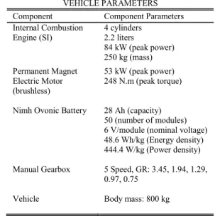
TABLE II VEHICLE PARAMETERS Component Component Parameters Internal Combustion Engine (SI) 4 cylinders 2.2 liters 84 kW (peak power) 250 kg (mass) Permanent Magnet Electric Motor (brushless) 53 kW (peak power) 248 N.m (peak torque) Nimh Ovonic Battery 28 Ah (capacity)
50 (number of modules) 6 V/module (nominal voltage) 48.6 Wh/kg (Energy density) 444.4 W/kg (Power density) Manual Gearbox 5 Speed, GR: 3.45, 1.94, 1.29,
0.97, 0.75
Vehicle Body mass: 800 kg
The inputs of the vehicle model are vehicle velocity,
and vehicle acceleration, . These inputs are provided by
the drive cycle defined for the system.
Since this is a bicycle model including the longitudinal dynamics only, vehicle mass is modeled as the half of the total vehicle mass. At the contact points between tires and the road there are reaction forces, and , due to the
gravitation, as shown in (1).
Longitudinal tire forces are produced with propulsion or braking action of the vehicle. There is a linear relationship, shown in equation (2), between the tire normal forces, obtained in equation (1), and maximum tire longitudinal forces, , which limit the tire friction forces. The road
friction coefficient, , is assumed to be uniform. In equation (2), denotes the actual friction forces between tire and
road. It should be noted that aerodynamic and grade resistances are neglected for simplicity of the analysis.
(1)
(2)
By using Newton’s second law we can find the relationship between vehicle acceleration and longitudinal tire force.
Fig. 1. Bicycle model used in [12]
(3) where is the net external longitudinal tire force and it is limited by the front and rear maximum longitudinal tire forces as shown in equation (4).
(4)
With equations (3) and (4) we can reach the limitation of the acceleration.
(5)
Before analyzing the tire normal forces the longitudinal dynamics is mentioned as a static system by considering the principle of d’Alembert.
(6)
By using equation (3) and (6) is found as shown in equation (7).
(7)
denotes the inertial force associated with accelerating/decelerating status of the vehicle.
Weight transfer under vehicle acceleration is modeled as shown in equations (8) and (9).
(8) (9) In equations (8) and (9) first terms on the right hand represent the static weight distribution and second terms represent the dynamic weight distribution.
B. Transfer Case Model
In our powertrain model front and rear axle torque values differ from each other. In order to split the torque between front and rear axles we need to use a center differential. In practical applications center differential may not be able to transfer all the produced torque to a single axle. This issue will be considered in the upcoming stages of our research. The transfer case model used in [2] is followed. The inputs of the model are total torque produced, inertia, rotational
speeds of the front and rear axles. The outputs are torque values of front and rear axles.
Output torque is calculated as shown in equation (10).
(10)
Front and rear torque values are determined via factor of torque split, , as shown in equations (11) and (12).
(11)
(12)
Factor of torque split, , is a function of rear rotational
speed ratio (RRSR), . This function,
, is to be the control law of the traction
controller. It will be determined after the dynamic programming procedure.
(13)
RRSR, , is calculated as shown in equation (14).
(14)
RRSR is the dynamic state of the model and it depends on the speed difference of front and rear axles. This ratio can be thought as the function of the slip of the vehicle and the aim of the traction controller is to make the RRSR value at 0.5, i.e. to make the slip zero.
The split factors of rear and front axles sum up to unity as shown in equation (15).
(15)
The output rotational speed is calculated as shown in equation (16).
(16)
The mean value of rotational speeds of front and rear axles,
, which is defined in equation (17), is used in equation
(16).
(17)
In equation (16), denotes the reduction in the transfer case model and it is taken as unity in our study.
III. DYNAMIC PROGRAMMING
As stated earlier dynamic programming is used to find an optimal path for controllers which are going to be designed. The aim of the dynamic programming is to minimize the weighted cost function. In our study these cost functions calculate the fuel consumption and wheel slip in energy management control and traction control systems respectively. The cost function is minimized over a finite horizon for a given drive cycle. The optimization problem can be formulated as shown in equation (18).
(18) Subject to (19)
where is the time-varying dynamics of the
plant, and is the time-varying cost of the plant. Dynamic state is denoted by , and control signal is denoted by .
There are initial and final constraints for the dynamic state of the system as shown in equations (20) and (21).
(20)
(21)
A. Energy Management
The optimization problem formulation in [3] is used in our study. The state-of –charge is the only dynamic state in the model. And torque split ratio between internal combustion engine and electric motor is the control signal. In [3], the discrete model is firstly defined as shown in equation (22).
(22)
In equation (22), stands for state-of-charge, stands for torque split ratio between internal combustion engine and electric motor, stands for vehicle velocity, stands for vehicle acceleration and stands for gear number.
For our DP analysis the discrete model in equation (22) is simplified as shown in equation (23).
(23)
where
(24) with
(25) and are defined as the state space and input space for the dynamic programming algorithm respectively in equation (25).
Here it is assumed that driving cycle is readily known. In our study FTP75 drive cycle is used for all simulations in order to have a fixed basis when comparing different controller schemes. Fig. 5 shows the velocity profile of the FTP75 drive cycle.
The optimization problem for energy management controller is formulated as shown in equation (26).
(26) Subject to (27)
In equation (27), is the fuel consumption
function of the HEV model as a cost of the system. Dynamic state, , is state-of-charge and control signal, , is torque split ratio between internal combustion engine and electric motor. The aim of the DP algorithm is to minimize the cost function.
TSR is defined as shown in equation (28).
(28) The working modes of the powertrain are given in Table III
TABLE III Powertrain Working Modes
TSR RANGE WORKING MODE
Electric Motor Only Mode
Torque Assist Mode
Engine Only Mode
Battery Charging Mode
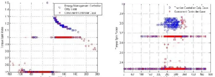
Initial charge is taken as 0.5 and final state-of-charge is between 0.5 and 0.51. For our DP analysis the algorithm outlined in [1] is used. We reach the optimal torque split ratio trace by taking the argument which minimizes the cost function given in equation (26). In Fig. 2, state-of-charge behavior is given and in Fig. 4, the optimal operating trace of the controller is given.
Fig. 2. SOC (left) and RRSR (right) behavior of systems
It can be seen in the results in Fig. 2 (left) and Fig. 3 (left) that the vehicle is working in the electric motor only mode in the low torque demand range when vehicle is launched. Optimal trace of the controller shows that in the low torque demand range except vehicle launch, recharging mode is preferred. Engine only mode is dominant in the middle torque demand range, and torque assist mode is preferred in the high torque demand mode. In Fig.3 (left), optimum trace shows that our hybrid electric model works like a typical parallel hybrid electric vehicle [5].
Fig. 3. Optimal Operating Points of Control Systems B. Vehicle Dynamics
The algorithm outlined in [1] is also used for DP analysis of vehicle dynamics control system. Here the vehicle is assumed to be non-hybrid so the battery and the electric motor are removed from the system. The only dynamic state is the rear rotational speed ratio (RRSR), . The
torque split factor between front and rear axles is the control signal.
The discrete model is firstly defined as shown in equation (30).
(30)
In equation (30), stands for RRSR, stands for torque split factor between front and rear axles, stands for vehicle velocity, stands for vehicle acceleration, stands for gear number and stands for the friction coefficient between tire and road.
For our DP analysis the discrete model in equation (30) is simplified as shown in equation (31).
(31)
where
(32) with
(33) and are defined as the state space and input space for the dynamic programming algorithm respectively in equation (33).
When simplifying the discrete model we have to know the friction coefficient between road and tire as well as vehicle speed, vehicle acceleration and gear number. For traction controller studies, the most common approach is to make simulations for short distances. In this study we need to use long drive cycles in order to provide the coherence between the two control problems. It is assumed that friction coefficient is given for the drive cycle. This is specified based on the limitation of the vehicle acceleration given in the equation (5).
The optimization problem for traction controller is formulated as shown in equation (34).
(34) Subject to (35)
In equation (35), is the wheel slip
function of the vehicle model as a cost of the system. Dynamic state, , is RRSR and control signal, , is torque split factor between front and rear axles. The aim of the DP algorithm is minimizing the wheel slip while maximizing the tractive force. TSF is defined as shown in equation (36).
(36) The boundaries for TSF are defined as shown in equation (29).
(37)
The working modes of the powertrain are given in Table IV. TABLE IV
Powertrain Working Modes
TSF RANGE WORKING MODE
Rear Axle Only Mode
Front and Rear Mixing Mode
Front Axle Only Mode
Initial RRSR is chosen as 0.5. The final RRSR value is between 0.5 and 0.51. RRSR behavior is given in Fig. 2 (right). Fig. 3 (right) shows the optimal operating trace of the controller.
Optimal trace of the controller shows that in the low speed range rear axle only mode is preferred. Front and rear axle mixing mode is dominant in the middle and high speed range. There are transitions between front and rear axle when crankshaft speed is about 250 rad/s.
C. Concurrent System
The problem formulation for concurrent case is shown in equation (38)-(40). In this part the control systems for energy management and vehicle dynamics are combined. The DP algorithm is arranged for two dynamic states, namely state-of-charge and RRSR. The state space and input space including the default values for concurrent optimization are the same as the individual processes.
(38) Subject to (39 (40)
It is important to note that the concurrent optimization formulation given in (38)-(40) contains the two automotive control problems that are coupled by nature and traditionally solved as separate problems. For example, our concurrent problem formulation reduces to the energy management problem formulation when the state variable of traction controller is kept fixed and vice versa. Fig. 3 (plus signs) shows the optimal traces of the concurrent controller. Torque assist mode got more dominant in the high torque demand range. Transitions between front and rear axles took place
between 200 rad/s and 350 rad/s range. It should be noted that we need a complex transfer case model in order to provide front/rear axle only modes. In this study the main objective is to obtain the optimal traces. Working mode of powertrain should also be considered when analyzing the results. In the torque assist mode, the decrease in wheel slip results in decrease in energy loss of the vehicle.
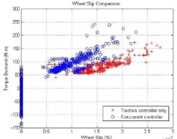
Fig. 4. Wheel slip comparison of concurrent and traction controllers
Fig. 5. Fuel rate comparison of concurrent and EM controllers TABLE V
Fuel Consumption Comparison over FTP75 Cycle Fuel Consumpti on (l/100km) Average Wheel Slip (%) Improvement FC AWS EM Only Case 8.3 TC Only Case 3.6 Concurrent Controller 7.5 3.4 9.63 % 5.5 % In Fig. 4 and Fig. 5, the fuel rate and wheel slip comparisons are illustrated between individual cases and concurrent. Our results indicate that fuel rate is decreased when concurrent controller is used since energy loss due to the slippage is eliminated by hybrid energy management strategies such as regenerative braking. The profile of concurrent controller stays around an optimum fuel rate line with low fluctuations. This tells us that power consumption of electric motor gets higher by being dominant in the torque assist mode of the powertrain and helping the internal combustion engine to operate in the fuel efficient range. The fuel rate and wheel slip profiles are integrated over FTP75 drive cycle given in Table V. The results indicate that we can obtain high levels of fuel efficiency in the long range driving conditions. Hard acceleration and braking ranges are outlined where the
difference is significant. Wheel slip is lowered for the same torque demand when concurrent controller is used since torque adjustment of wheel slip controller is stabilized by the energy management strategy. As electric motor assistance is improved the contribution of electric motor gets higher. This makes the torque transitions of the powertrain stable.
IV. CONCLUSION
In this study the DP is applied for three different controller problems and promising results of the concurrent system are achieved. Comparisons show us the results of concurrent controller are better. Concurrent system provides interaction between energy management and traction controllers. Knowing the road conditions is an advantage for energy management strategy whereas knowing the torque transitions of power suppliers is an advantage for the traction controller. These advantages make the concurrent solution work better than the controllers operating separately. The results of concurrent controller in this study motivate us to study on designing concurrent controllers in our research.
REFERENCES
[1] European Environment Agency, “Transport and environment: on the way to a new common transport policy”, in EEA Report, no:1/2007. [2] D., Kim, S., Hwang and H., Kim, “Vehicle Stability Enhancement of
Four-Wheel-Drive Hybrid Electric Vehicle Using Rear Motor Control”, in Vehicular Transactions on Vehicular Technology, vol. 57, no. 2, March 2008.
[3] S., Delprat, J., Lauber, T., M., Guerra and J., Rimaux, “Control of a Parallel Hybrid Power train: Optimal Control,” in IEEE Trans. Veh. Technol., vol.53, no.3, pp.872-881, May 2004.
[4] F. Borelli, A. Bemporad, M. Fodor and D. Hrovat, “An MPC/Hybrid System Approach to Traction Control”, in IEEE Trans. on Con. Sys. Technol., vol. 14, no.3, May 2006.
[5] O., Sundström and L., Guzzella, “A Generic Dynamic Programming Matlab Function”, In Proceedings of the 18th IEEE International Conference on Control Applications, pages 1625-1630, Saint Petersburg, Russia, 2009
[6] O., Sundström, L., Guzzella and P., Soltic, “Optimal Hybridization in Two Parallel Hybrid Electric Vehicles using Dynamic Programming”, in 17th IFAC World Congress, ser. Proc. of the 17th IFAC World Congress, Seoul, Korea, 2008.
[7] A., Sciarretta, L., Guzzella, “Control of Hybrid Electric Vehicles,” in IEEE Cont. Sys. Mag., Apr. 2007.
[8] Y., Huang, C., Yin, J., Zhang, “Optimal Torque Distrubution Control Strategy for Parallel Hybrid Electric Buses”, in WSEAS Transactions on Systems, vol.7, issue 6, June 2008.
[9] A., I., Antoniou, A., Emadi, “Adaptive Control Strategy for Hybrid Electric Vehicles”, in IEEE Electric Power and Power Electronics Center.
[10] C., Lin, H., Peng, J., W., Grizzle and J., Kang, “Power management strategy for a parallel hybrid electric truck”, in IEEE Transactions on Control Systems Technology, vol. 11, no. 6, November 2003. [11] A. Rousseau, “PSAT Training Part 05”, Argonne National Laboratory.
[Online]. Available:
http://www.transportation.anl.gov/pdfs/HV/406.pdf, September 2011 [date accessed].
[12] N., J., Schouten, M., A., Salman, N., A., Kheir, “Fuzzy Logic Controller Parallel Hybrid Vehicles,” in IEEE Trans. Veh. Con. Sys. Technol., vol. 10, no.3, May 2002.
[13] K. Tong, “Simultaneous Plant/Controller Optimization of Traction Control for Electric Vehicle”, University of Waterloo, Ontario, Canada, 2007.