Cite this article as: Soltanbeigi, B., Altunbas, A., Gezgin, A. T., Cinicioglu, O. "Determination of Passive Failure Surface Geometry for Cohesionless Backfills", Periodica Polytechnica Civil Engineering, 64(4), pp. 1100–1110, 2020. https://doi.org/10.3311/PPci.14241
Determination of Passive Failure Surface Geometry for
Cohesionless Backfills
Behzad Soltanbeigi1, Adlen Altunbas2, Ahmet Talha Gezgin3, Ozer Cinicioglu3*
1 Institute for Infrastructure and Environment, University of Edinburgh, Thomas Bayes Road, EH9 3JL Edinburgh, UK
2 Department of Civil Engineering, Faculty of Engineering and Natural Sciences, Istanbul Medipol University, 34810 Beykoz, Istanbul,
Turkey
3 Department of Civil Engineering, Faculty of Engineering, Bogazici University, 34342 Bebek, Istanbul, Turkey * Corresponding author, e-mail: [email protected]
Received: 28 April 2019, Accepted: 09 July 2020, Published online: 18 August 2020
Abstract
Correct determination of the passive failure surface geometry is necessary for the design of retaining structures. The conventional theories assume linear passive failure surfaces even though it is known that the actual failure surfaces are non-linear. Many researchers claimed the appropriateness of a hybrid curved-linear method. This approach estimates the curved section by a log-spiral function, which then connects to the backfill surface with the conventional linear assumption. The main drawback here is that the geometric properties of the hybrid mathematical function is not directly related to the mechanical properties of soils. Thus, this study attempts to provide a mechanical description for the assumed geometrical parameters. For this purpose, a series of 1 g small scale retaining wall model tests, simulating passive failure, are conducted on two different backfill soils. The relative density is varied in the model tests and the resultant peak friction angles of the backfills are calculated as functions of failure stress state and relative density using a well-known empirical equation. Transparent sidewalls allow for visualization of the failure surface evolution, which is obtained by capturing images and analysing then through Particle Image Velocimetry (PIV) technique. Subsequently, the quantified slip zones are fitted with the hybrid curved-linear approach. The relationships between the peak friction angle and the geometrical characteristics of the best-fit log-spiral and linear functions are investigated. Obtained results are used to propose a set of equations that allow the estimation of non-linear passive failure surfaces as function of peak friction angle.
Keywords
passive state, particle image velocimetry (piv), dilatancy, retaining wall, physical modelling
1 Introduction
Identification of the geometries of failure surfaces that emerge in backfills has critical importance in the anal-ysis and design of retaining structures [1]. In the prac-tice of geotechnical engineering, generally Coulomb [2] and Rankine [3] theories are used in design. Both theo-ries are based on simplified assumptions regarding the geometry and orientation of the backfill failure surfaces. The common fundamental hypothesis of both theories is that the shear plane formed in the backfill at the ulti-mate state is a straight line, the inclination of which is only a function of the internal friction angle of the back-fill. Several studies in literature investigated the evolution of lateral pressures and the formation of shear bands in retained backfills. Some of these used experiments [4–11] whereas the others preferred numerical methods [12–18].
One common outcome of all studies on the subject is that effective strength parameters (cohesion, soil friction angle, or soil-wall interface friction angle) control the magnitude of passive pressure [7]. This is expected since the problem involves a limit state problem. Additionally, several researchers noticed other influencing factors that control the magnitude of lateral thrust, such as: backfill density [19], pressure level [19] and dilation angle of back-fill soil [19–21].
On the other hand, the results of all these studies sug-gest that the geometries of slip surfaces that emerged in retained backfills at failure are nonlinear. In the lit-erature, factors affecting the geometries of passive fail-ure surfaces are as following: internal friction angle [22, 23], interface friction angle [23], backfill density [19].
Regarding the mathematical form of the nonlinear fail-ure surface, researchers generally suggested a composite form including both linear and logarithmic spiral sections [7, 12, 23, 24].
Liu et al. [25] suggested a modified method to obtain the failure surface geometry and earth pressure coefficient for passive state of failure. The proposed approach is based on the logarithmic spiral method developed by Terzaghi [24]. To find the corresponding angle of the logarithmic spiral (which determines the characteristics of the spiral), a math-ematical solution is used (i.e. using the bisection method for root-finding). Additionally, for a backfill without sur-face inclination, it is assumed that linear portion of the failure surface meets the backfill surface with an angle of
π/4 – ϕ'/2 (i.e. Rankine zone). Successively, the proposed
method is verified by using FEM numerical approach. Overall, it is shown that obtained results from the proposed method are in agreement with those of FEM simulations.
Xu et al. [26] proposed an analytical approach to esti-mate the stress state within a retained backfill. In this method, a log-spiral failure surface is assumed, which is discretized into dices. Then, the forces acting on each dice (depending on its location, within or at the boundary of the log-spiral region), allowing observation of local internal forces distribution. The inter-dice normal and shear forces are obtained through considering integration of the rela-tionships gained by satisfying the force and momentum equilibrium. This method is verified by FEM simulations, and it is pointed out that the normal and shear stresses obtained from both methods are similar in most parts of the backfill (except near the wall boundary).
Unfortunately, none of these studies offered a practical guidance by which the geometrical characteristics of the logarithmic spiral failure surface can be obtained. All sug-gestions were left at the level of identifying the suitability of using logarithmic spiral form as a good fit to the passive failure surfaces.
This study attempts to address this deficiency by link-ing the geometrical characteristics of logarithmic spiral to the properties of backfill soils. From mentioned pre-vious studies, it is deduced that peak friction angle can be referred as a global parameter that encompasses the influences of other affecting factors. The peak friction angle (ϕp') is a combined outcome of critical state friction
angle (ϕc') and peak dilatancy angle (ψp) [27–31]. As ψp is dependent on the collective influences of backfill den-sity and pressure level [31], and ϕc' is a soil constant, ϕp'
embodies the joint influences of all influential parameters
listed above. That is why the goal of this study is to devise a method which mathematically defines logarithmic spi-rals to fit passive failure surfaces as functions of backfill peak friction angles.
For this purpose, small scale retaining wall model tests are conducted with two different sand types. This study is limited to the investigation of vertical retaining systems that translate horizontally under plane strain conditions. Wall rotation and different wall geometries are out of the scope of this study as this is the first attempt at linking the geometrical characteristics of logarithmic spiral functions to measurable soil properties. Well-known empirical equa-tions from literature are used to calculate the peak friction angles of model backfills as functions of density and fail-ure stress state. PIV method is employed to visualize and determine the geometries of failure surfaces. As a result, it became feasible to investigate the influence of ϕp' on the
geometrical characteristics of failure surfaces. Finally, an empirical method, by which the geometries of passive fail-ure surfaces can be accurately predicted, is presented. 2 The retaining wall model
To investigate geometries of failure surfaces, 1 g small scale retaining wall model tests are conducted. In each model test, backfill soil is prepared at a different relative density (ID). Under 1 g conditions, the magnitude of backfill soil's
ϕp' directly changes with the changes in relative density.
This way, it becomes possible to monitor the influence of ϕp'
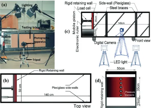
on failure surface geometry. Physical model set-up consists of a testing box, a model retaining wall that is capable of only translating laterally, a sand pluviation system, a stor-age tank, a crane, and a data acquisition system, as shown in Fig. 1(a). The testing box is, 140 cm in length, 60 cm in depth, and 50 cm in width, as illustrated in Fig. 1(b) and Fig 1(c). Sides of the box are made of 20 mm thick Plexi- glas allowing the observation and monitoring of soil defor-mations. To maintain plane-strain conditions at all stages of the test, it is necessary to prevent lateral deflections of Plexiglas side walls. For this purpose, model frame is equipped with metal braces supporting the Plexiglas side walls (Fig. 1(a)). Though the braces obstruct a small portion of the view when photographs of the tests are captured, this in no way hinders the identification of the failure surface geometry. Through the transparent side walls, photographic images of the backfill at different stages of wall deforma-tion can be captured for examinadeforma-tion. Obtained images are analyzed using PIV method, which led to visualized pas-sive failure surfaces [32–36]. The model retaining wall is an
aluminium plate with rectangular cross-section. The height and width of the model wall are 35 cm and 50 cm, respec-tively. To minimize the adverse effects of the rigid bound-ary at the bottom, the moving plate that simulates the ver-tical retaining wall is located 15 cm above the bottom of the test box. An electrical motor-actuator system drives the model wall laterally either towards or away from the retained backfill. The displacements of the wall are mea-sured by an electronic ruler. Motor displacement steps are used to validate the measurements of the electronic ruler. Fig. 1(d) shows five sensitive miniature pressure transduc-ers mounted along the vertical axis of the model wall for observing the variations of lateral earth pressures along the face of the wall. Density cans are buried in the back-fill during model preparation stage at the further end of the box away from the model wall. This way these cans do not interfere with the evolution of failure surfaces and they provide the means to measure backfill density after the completion of model tests. Variations of vertical stresses within the backfill are calculated using the measurements of the density cans. To verify vertical stress calculations, two miniature pressure transducers are buried in the backfill during model preparation stage of each test (Fig. 1(b) and Fig. 1(c)). A multi-channel data logger system is used for collecting data. Data logger is capable of handling an aggre-gate data collection rate of 400 kHz, with a maximum per channel sample rate of up to 500 Hz which is more than suf-ficient considering the velocity of model wall movement.
3 Calculation of peak friction angle of backfill soils The goal of this study is to link the geometrical charac-teristics of failure surfaces to backfill soil's ϕp'. Therefore,
it is necessary to know the magnitude of ϕp' once the
back-fill is prepared. This is not an easy task as ϕp' varies with
pressure, density, stress path and loading conditions. It is not possible to prepare equivalent samples of backfill soils for strength testing. Even though the sample is prepared with the same relative density as the model, changes in the symmetry conditions (axisymmetric versus plane strain), stress state or stress path will result in the deviation of the measured values from the model values. Therefore, an alternative method is necessary to obtain the values of ϕp'
that prevail in the backfill. For this purpose, well-known empirical equations, available in literature, are used to determine ϕp'. First of these equations are given in Eq. (1)
and relate ϕp' to ϕc' and ψp' of the backfill soil.
φp' =φc'+rψp (1) Here, r is an empirical line-fitting parameter. ψp is also referred as the maximum rate of dilatancy and it is mea-sured at the instance of peak failure. The relationship given in Eq. (1) was first described by Bishop [27] and later formulated by Bolton [28] in its final form. The mag-nitude of r is dependent on sample symmetry conditions. Second empirical equation (Eq. (2)) allows the calcula-tion of ψp as a function of backfill relative density (ID) and mean effective stress at failure (pf') [28]:
ψ ψ ψ p R D f a A r I A r I Q ln p p R = = − − 100 ' . (2)
Here, Q, R and r are empirical line-fitting parameters that depend on inherent soil characteristics and pa is the atmospheric pressure. The values of Q and R for the test-ing sand are obtained by triaxial testtest-ing. Chakraborty and Salgado [30] suggested that the value of the parameter Q depends on the magnitude of initial confining stress (pi') of
the soil. The results of the triaxial tests conducted for this study supported the findings of Chakraborty and Salgado [30]. Following Chakraborty and Salgado [30], the magni-tude of Q can be calculated using Eq. (3):
Q= +η β ln ' . pi (3)
Here, β and η are soil-specific empirical line-fitting parameters. Chakraborty and Salgado [30] showed that Eq. (3) is suitable for stresses that range from low to inter-mediate. The pi' values of the triaxial tests of this study
range from 25kPa to 500kPa and the soil specific values of the parameters β, η, and R are obtained for the two soils used. Values of these parameters for both soils used in this study are given in Table 1. It is known that ψp is indepen-dent of sample symmetry conditions [28, 37]. Therefore, at the same stress state, identical ψp values are measured in plane strain and triaxial tests. Consequently, it is possible to calculate ψp of the model backfill using the line-fitting parameters obtained by triaxial testing.
On the other hand, it is known that the values of ϕp'
measured under axisymmetric and plane strain conditions differ [37–39]. According to Schanz and Vermeer [37], this difference is caused by the dependence of ϕp' on
den-sity and stress path. Since the stress path under axisym-metric and plane strain conditions diverge, measured ϕp'
values also differ. That is why, ϕp' values are calculated
with Eq. (1), which uses line-fitting parameters suitable for axisymmetric conditions, are converted into ϕp' values that
are relevant for plane strain conditions. This is achieved using a method proposed by Hanna [39]. The r values rel-evant for axisymmetric and plane strain conditions for both backfill soils are given in Tables 1 and 2. Inserting the values of ψp (calculated using Eq. (2)), ϕc' of the soil
and r value (specific to plane strain condition) into Eq. (1), the magnitude of plane strain ϕp' can be calculated. Once
the value of ϕp' is obtained for each model test, it becomes
possible to investigate the influence of ϕp' on failure
sur-face geometry.
Apparently, Eq. (2) requires the input of pf'. The
mag-nitude of pf' is measured at the instance of failure using
the pressure transducers. Available transducers measure the normal stress in the vertical direction and in the hor-izontal direction normal to the wall. As a result, the nor-mal stress in the orthogonal horizontal direction must be calculated. The model box conforms to plane strain condi-tions. Therefore, at-rest conditions prevail in the direction of the normal to the sidewall. Accordingly, normal stresses in the direction of the sidewall normal are assumed to be equal to the measured lateral earth pressures before the occurrence of any deformation.
4 Backfill properties and sample preparation
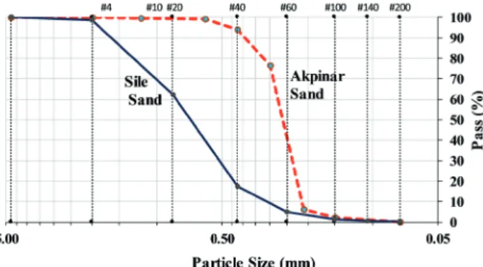
Two different sand types are used in this study; these are Akpinar (S1) and Sile (S2) sands which are obtained from different regions around Istanbul. S1 and S2 sands are poorly graded according to United Soil Classification System (USCS), see Fig. 2.
A summary of the physical characteristics of the sands are given in Table 1. Particle shape characteristics are quantified based on the grain shape charts proposed by Cho et al. [40].
Direct shear tests are conducted to measure the inter-face friction angle between the model wall and the back-fill sand. Measured backback-fill model-wall interface friction angles vary between 18° (loosest) and 24° (densest) for S1 and S2 sands.
It must be noted that in the current study the model wall material is the same in all tests. The underlying reason for this choice is that in practice the interface friction can vary within a limited range for sand backfills. For inter-face problems in sands, the roughness of a surinter-face is typ-ically quantified by the normalized roughness ratio which is the ratio of maximum roughness to mean grain diame-ter (D50) [41]. Maximum roughness is defined as the maxi-
mum vertical distance between a peak and a trough of the surface over a length equal to the mean grain diameter. However, following the definition of roughness, in practice it is impossible to have retaining wall surfaces that are per-fectly smooth/rough. Accordingly, considering the inter-faces between sand-sized grains and retaining structures (constructed with modern tools and materials), expected interface friction angle is unlikely to exceed the range of variation that was proposed by Terzaghi [24]. He sug-gested that the magnitude of interface friction angle varies between one-third and two-thirds of for practical applica-tions. The obtained interface friction angles for this study are also within this range.
Low friction transparent high-density polyethylene sheets are applied on the plexiglass side walls to satisfy plane-strain conditions. In order to investigate the influ-ence of soil friction angle on the geometry of passive fail-ure surface, tests are conducted with backfills that have different peak friction angles. This is achieved by prepar-ing the backfill soils with different relative densities.
Model backfills are prepared by dry-pluviation. Pluviation height is adjusted to achieve different relative densities. Whenever the target relative density cannot be reached by pluviation only, a hand-held electric compac-tor is used to compact the backfill in layers. Cinicioglu and Abadkon [31] showed that neither ψp nor ϕp' are influenced
by overconsolidation ratio (OCR). As a result, Eq. (1) and
Eq. (2) can still be used to calculate the magnitude of ϕp'
for the model backfill. As soon as a test is completed, density cans buried in the backfill are extracted and weighed. The results are used for calculating back-fill relative density and to check backback-fill homogeneity. Insignificantly small variations in vertical stresses under 1 g conditions justify the assumption of uniform ϕp' for the
whole model. Passive failure of backfill is simulated by horizontally translating the model wall toward the back-fill. Since, the tests are conducted with dry sand, there is no rate effect influencing soil response. Thus, based on the image-capturing rate of the camera, the translation speed of the model wall is adjusted (0.5 mm/s), which ensures the image quality level (i.e. resolution).
5 Failure surface geometry by PIV
In this study, PIV is used for monitoring the evolution of the backfill deformation caused by the translation of the model wall. GeoPIV-RG, a MATLAB based PIV software, specifically utilized for geotechnical applications, is used for the analyses of the images captured during the tests. Detailed information regarding GeoPIV-RG algorithms can be found in Stanier et al. [42]. PIV method is a popular approach to detect the deformations in soil medium [43].
The utilized camera can capture four images per sec-ond. This rate is enough for monitoring the quasi-static deformations of the model backfill. In all tests, the camera is placed at a fixed distance from the wall and the model is illuminated using special projectors to ensure the highest image quality.
Cumulative shear strain maps for different stages of the tests are obtained from the GeoPIV-RG analyses. Strain maps, corresponding to the instance of passive fail-ure, for each test are color-coded based on strain magni-tude. The high visual contrast achieved in these images makes it easier to distinguish the passive failure surfaces. In order to quantify the geometries of discerned failure surfaces, a coordinate system is established. The vertical axis of the coordinate system is coincident with the ini-tial position of the model wall and the origin is located at the bottom of the wall. Using this coordinate system, coordinates of the points along the failure surface that correspond to outer edge of failure surface are digitized. All coordinate measurements are done with respect to the position of the wall before any displacement. In order to achieve unit-independent quantification, measured coor-dinates of the failure surface are normalized by height of the model wall (Hw).
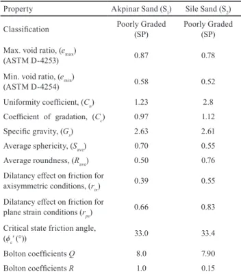
Table 1 Mechanical Properties of Akpinar and Sile Sands
Property Akpinar Sand (S1) Sile Sand (S2)
Classification Poorly Graded (SP) Poorly Graded (SP) Max. void ratio, (emax)
(ASTM D-4253) 0.87 0.78
Min. void ratio, (emin)
(ASTM D-4254) 0.58 0.52
Uniformity coefficient, (Cu) 1.23 2.8
Coefficient of gradation, (Cc) 0.97 1.12
Specific gravity, (Gs) 2.63 2.61 Average sphericity, (Save) 0.70 0.55
Average roundness, (Rave) 0.50 0.76
Dilatancy effect on friction for
axisymmetric conditions, (rtx) 0.39 0.55
Dilatancy effect on friction for
plane strain conditions (rps) 0.66 0.83 Critical state friction angle,
(ϕc' (°))
33.0 33.4
Bolton coefficients Q 8.0 7.90 Bolton coefficients R 1.0 0.15
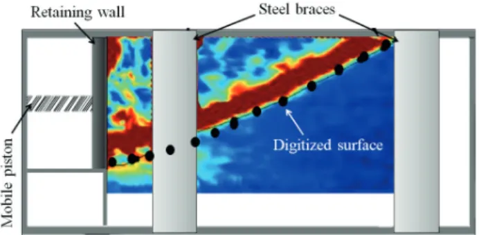
The presence of the braces that are necessary for sat-isfying plane strain conditions partially blocks the view of the failure surface geometry. However, braces are essential to prevent the bulging of plexiglass during soil deformation. However, failure surface geometry is clearly discernible, and the obstructed portion can be easily inter-polated as observed in Fig. 3.
6 Determination of failure surface geometry
Based on the results of PIV analyses, geometries of failure surfaces are determined in all model tests for both sand types, as shown in Fig. 4. Evident from all results, geom-etries of all passive slip planes are nonlinear and link the toe of the rigid retaining wall to the surface of the cohe-sionless backfill. It is clear that the magnitude of peak fric-tion angle, which is obtained through peak dilatancy angle, influences the shapes of failure surfaces. Additionally, the failure surfaces emerge at the ground level in the order of their respective ϕp' magnitudes. In other words, higher
magnitudes of ϕp' results in greater Bf values. 7 Prediction of slip plane geometry
As explained in the introduction section, several researchers suggested the suitability of using logarithmic spiral as the mathematical function to define the shapes of passive failure
surfaces in cohesionless soils [7, 12, 23, 24]. However, the current approach to define the log-spiral failure surface is based on predefined assumptions, which then follows a trial and error procedure. Accordingly, an ideal approach, which provides the geometrical characteristics of logarith-mic spiral failure surfaces as a function of soil properties is still lacking in the literature. Therefore, this study attempts to cancel the necessity for the prevailing assumptions, which would enhance the accuracy of passive failure sur-face predictions. To this end, the geometrical characteris-tics of the slip plane are correlated with the backfill peak friction angle. This is achieved by fitting logarithmic spi-rals to experimentally determined passive failure surfaces and then investigating the correlation between backfill ϕp'
and the geometrical characteristics of the logarithmic spi-rals that best fit the determined failure surfaces.
Experimentally observed passive failure surfaces can be divided into spiral and linear sections. The linear sec-tion is an extension of the spiral part (Fig. 5). Assuming that the spiral portions of passive failure surfaces have log-arithmic spiral forms, Terzaghi et al. [44] suggested that the log-spiral that yields the smallest total passive resis-tance corresponds to the actual passive failure surface. To find this failure plane, Terzaghi et al. [44] explained the necessary steps and assumptions as given below:
For cohesionless soils at passive limit state, a force equilibrium must exist between PP (resultant of the nor-mal and frictional components of the passive earth pres-sure), the weight of the area ABCD (see Fig. 5) and the fric-tional resistance due to the weight. It is also assumed that PP acts at lower third of AD (i.e. wall height). Additionally, following assumptions are made to obtain the composite passive failure surface (linear and curved portions):
Fig. 3 Determination of the failure surface geometry as plotted on the
cumulative shear strain map (for S2 sand with )
Fig. 4 Geometries of passive failure surfaces obtained from PIV
The linear part (BC) makes π/4 – ϕ'/2 with the horizon-tal surface of the backfill. The curved section is tangent to the linear part at B, and the center of spiral passes through
DB, which also makes π/4 – ϕ'/2 with the horizontal
sur-face of the backfill (an isosceles triangle is formed above
ABD curved wedge).
The curved lower part of failure surface (AB) is an arc of a logarithmic spiral, defined as:
r r e= 0 θtanφ
,
' (4)
where, r0 is the initial radius of the spiral (OA), θ is the spiral angle (angle between r and r0), O is the pole of the spiral located along the BD line (can be out of the zone defined by the limiting points B and D) (Fig. 5).
To compute PP, the sliding surface ABC composed of spiral (AB) and linear (BC) sections is defined. This is done by varying the position of the pole of the spiral along the line BD (referred as the s-line). This iterative process is continued until the desired failure surface that yields the smallest total passive resistance is obtained. However, this proposed graphical solution needs considerable time and effort. On the other hand, accuracies of the failure surfaces obtained by considering the abovementioned assumptions, have never been validated by model tests. Accordingly, in the next section, attempt has been made to evaluate the applicability of the log-spiral method for defining slip surface geometries using model test results. Following, possible relationships between the defining geometrical characteristics of the experimentally obtained best-fit spiral functions and ϕp' will be examined.
7.1 Necessary steps for plotting the best-fit log-spiral failure surface
Fitting the experimentally obtained failure surfaces with log-spirals requires the identification of two unknowns,
α and θ0. Here, α is the angle that forms between the line BC and the horizontal, and θ0 is the angle that forms between the line OA and the vertical, as shown in Fig. 5. One of the main assumptions for the determination of the log-spiral is that the final radius of the log-spiral (OB) must make an angle equal to α with the free surface of the backfill (passing through top of the wall). The origin of log-spiral O is located on OB line as well. PIV analyses of the model tests visually reveal the value of α. Since α is obtained experimentally, iteration is necessary only for determining the value of θ0, which determines the loca-tion of O (Point O lies at the intersecloca-tion of the extension of the line BD and the line that starts at point A making the
angle θ0 with the vertical). Each iteration requires several steps to plot the log spiral and the linear portion. This is performed by a script in MATLAB.
Experimentally obtaining the value of α and assuming a value for θ0, the value of θ and η are obtained as follows: θ=90°−θ −α
0 , (5)
η=180°− −α θ. (6) Then, it is possible to obtain lengths of FD, OD, OF,
GF, OG, and FA using the geometry of the problem given
in Fig. 5. Accordingly, length of r0 is obtained as:
r OF FA0= + . (7)
Inserting OF and FA into Eq. (7):
r0 HW 0 0 1 =
( )
( )
( )
+( )
tan sin sin cos . θ α θ θ (8)Location of O defined by OJ and JA, which is obtained using r0 and θ0:
OJ r= 0cos
( )
θ0 , (9)JA r= 0sin
( )
θ0 . (10)Having r0 and O, it is now possible to determine the log-spiral part of the failure surface. This requires replac-ing θ by i values (0< i < θ). Every gradual increase in i results in a new radius for the spiral (rn) and ultimately when i = θ, rn will be equal to rf. Coordinates for the end point of rn is calculated through:
Y ri= 0cos
( )
θ0 −(
rncos(
θ0+i)
)
, (11) Xi=rnsin(
θ0+i GD)
− , (12) Where, GD H= W( )
( )
( )
( )
+ tan sin sin sin . θ α θ θ 0 0 1 (13)Having the coordinates of B(Xf,Yf), it is possible to plot the linear portion as well. Fig. 6 visually explains the influence of θ0 on the resulting failure surfaces.
8 Results
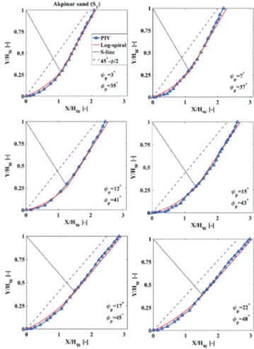
The failure surfaces, determined experimentally through PIV analyses, are fitted with log-spiral functions. The results are presented in Fig. 7 and Fig. 8 for model tests with S1 and S2 sands, respectively. The magnitudes of backfill ϕp' and ψp are reported in the legends of each figure.
Evidently, it is necessary to know the magnitudes of the parameters θ and α for plotting the linear and curved portions of the predicted failure surfaces. Therefore, this study attempts experimentally to examine the dependence of the necessary unknown fitting parameters (i.e. θ and α) on ϕp'. Experimentally obtained variations of θ and α are
shown in Fig. 9 for both S1 and S2 sands.
From Fig. 9, it is noticed that the variations of all examined parameters (θ and α) with ϕp' are linear for
both sands. In case of α – ϕp' relationship, experimentally
obtained relat-ionships are inversely linear for both sands (Fig. 9(a)) and are given in Eq. (14) for S1 sand and in Eq. (15) for S2 sand:
αS1=62°−0 8. φp' , (14) αS2=59°−0 8. φp'.
(15)
Fig. 6 Influence of the unknown parameter θ0 on the resulting failure
surface (for a backfill with ϕp' = 30°)
Fig. 7 Fitting experimentally visualized failure surfaces with log-spiral
function (for S1)
Fig. 8 Fitting experimentally visualized failure surfaces with log-spiral
function (for S2)
Fig. 9 Variation of fitting parameters with ϕp' (for the best fitting
Noticeable in Eqs. (14) and (15), the slopes of α – ϕp'
are the same for both soils and their zero-intercepts only slightly differ. The forms of the experimentally obtained
α – ϕp' relationships are the same as the commonly used α = 45° – ϕp'/2 relationship in literature [2, 3], whereas the values of their zero-intercepts and slope differ.
Additionally, experimentally obtained variations of θ0 with ϕp' for both soils are presented in Fig. 9. The results
point to a linear relationship as given in Eq. (16). θ0=φ +5
°
p' (16)
The results provided linear correlations between peak friction angle and the unknown fitting parameters (θ, θ0 and α). Additionally, r0 is also defined as function of HW,
θ0 and α. Thus, the general log-spiral function can be sug-gested in the new form as:
r H= W
( )
( )
e fp( )
+( )
(
)
tan sin sin cos . tan( ) θ α θ θ θ 0 0 1 ' (17) The proposed equation is unique, since it only uses peak friction angle as the input parameter to estimate the failure surface geometry under passive state.9 Discussion
As shown in the previous section of this paper, geometri-cal characteristics of passive failure surfaces are obtained for two different soils for a range of relative densities. The premise of this paper is that the geometrical charac-teristics of failure surfaces are linked directly to the mag-nitude of ψp (failure surface geometry is dependent on den-sity and stress state and because peak dilatancy angle (ψp) embodies the combined effects). However, determination of ψp is not very straightforward in practice. That is why the soil parameter to link to the failure surfaces' shape is chosen as the peak friction angle (ϕp').
The determination of ϕp' is common practice and is done
in almost all projects. Moreover, ϕp' is a direct function
of ψp as shown in Eq. (1). Obtained results supported the proposition regarding the dependence of failure sur-face geometries on ϕp' and the results are shown in Fig. 9.
The necessary geometrical features of a passive failure surface are defined as a function of θ and α, of which both vary linearly with ϕp'.
Additionally, when the results obtained from S1 and S2 sands are compared, it is noticed that the variations of θ and α with ϕp' are very similar. This suggests a direct dep-
endence of passive failure surface geometry on ϕp' which
requires further studying. Especially, because both back-fill soils used in model tests are poorly graded, tests on a well-graded soil will give valuable information regard-ing the influence of gradation characteristics on the geom-etry of failure planes. Another possible influence on pas-sive failure geometry is the mode of wall movement. This study used model tests which involve lateral transla-tion of a rigid wall. However, in problems where the wall rotates or deforms, the resulting passive failure geometry will most likely change.
On the other hand, it is necessary to note that all the mentioned shortcomings also apply to conventional methods of failure surface geometry prediction, such as Coulomb [2] or Rankine [3]. Fig. 7 and Fig. 8 also include comparisons with the conventional passive failure surface predictions. Evidently, linear failure surface predictions are significantly different from the experimentally deter-mined passive failure surfaces. Therefore, the use of new form of log-spiral function (Eq. (17)), for determining pas-sive failure surface geometries for cohesionless backfills, will result in more accurate predictions.
10 Conclusions
The classical theories on passive failure planes assume planar surfaces. However, as explained in the introduc-tion secintroduc-tion of this paper, the curved nature of failure sur-faces is well-known by researchers. However, approaches for mathematically defining the curved forms of passive failure surfaces are still lacking. Several researchers have noticed the suitability of log-spiral function for defining passive failure surfaces, but without linking the geomet-rical characteristics of the failure surfaces to the mechan-ical properties of backfill soils [16, 25]. This is attempted in this study through the use of model tests. The mechan-ical parameter for identifying the failure surface geom-etry is selected as the peak friction angle since it blends the influences of backfill density and stress state. Model tests are conducted with two different sands at different relative densities corresponding to different peak fric-tion angles. Failure surfaces are determined using Particle Image Velocimetry (PIV) analyses.
Based on the results, it is seen that the passive fail-ure surfaces are non-linear for both sand types and at all density levels. For dense backfills with higher ϕp',
result-ing failure surfaces extend further away from the model wall. Additionally, obtained failure surfaces are fitted with a log-spiral function. It is noticed that log-spiral functions fit the experimentally determined failure surfaces with
high accuracies. On the other hand, the linear failure sur-faces proposed by classical theories depart significantly away from the actual failure surfaces.
When the variations of geometrical characteristics of experimental failure surfaces with ϕp' are investigated, it is
noticed that the relationships are all linear. Consequently, obtained results suggest that log-spiral method can pre-cisely predict the passive pressure failure surface geometry.
Moreover, using the results presented in this study, it is possible to define log-spiral passive failure surfaces using
ϕp' as the only input parameter.
Acknowledgement
Authors would like to thank the Scientific and Technological Research Council of Turkey (TUBITAK Project 114M329) for providing financial support.
References
[1] Salgado, R. "The Engineering of Foundations", 1st ed., McGraw-Hill, Boston, MA, USA, 2008.
[2] Coulomb, C. "Essai sur une application des regles des maximis et minimis a quelues problemes de statique relatifs a larchitecture" (Test on an application of the rules of maximis and minimis to some problems of statics relating to architecture), In: Memoires de mathematique et de physique, Presentes a l'Academie Royale des Sciences, Paris, France, 1776, pp. 343–382. (in French)
[3] Rankine, W. J. M. "II. On the Stability of Loose Earth", Philosophical Transactions, 147(84), pp. 9–27, 1857.
https://doi.org/10.1098/rstl.1857.0003
[4] Hansen, J. B. "Earth Pressure Calculation", The Danish Technical Press, Copenhagen, Denmark, 1953.
[5] Narain, J., Saran, S., Nandakumaran, P. "Model Study of Passive Pressure in Sand", Journal of the Soil Mechanics and Foundation Division, 95(4), pp. 969–984, 1969.
[6] Rowe, P. W., Peaker, K. "Passive Earth Pressure Measurements", Géotechnique, 15(1), pp. 57–78, 1965.
https://doi.org/10.1680/geot.1965.15.1.57
[7] Duncan, J. M., Mokwa, R. L. "Passive Earth Pressures: Theories and Tests", Journal of Geotechnical and Geoenvironmental Engineering, 127(3), pp. 248–257, 2002.
https://doi.org/10.1061/(ASCE)1090-0241(2001)127:3(248) [8] Wilson, P., Elgamal, A. "Large-Scale Passive Earth Pressure
Load-Displacement Tests and Numerical Simulation", Journal of Geotechnical and Geoenvironmental Engineering, 136(12), pp. 1634–1643, 2010.
https://doi.org/10.1061/(ASCE)GT.1943-5606.0000386
[9] Tajabadipour, M., Marandi, M. "Effect of rubber tire chips-sand mixtures on performance of geosynthetic reinforced earth walls Effect of Rubber Tire Chips-Sand Mixtures on Performance of Geosynthetic Reinforced Earth Walls", Periodica Polytechnica Civil Engineering, 61(2), pp. 322–334, 2017.
https://doi.org/10.3311/PPci.9539
[10] Chogueur, A., Abdeldjalil, Z., Reiffsteck, P. "Parametric and Comparative Study of a Flexible Retaining Wall", Periodica Polytechnica Civil Engineering, 62(2), pp. 295–307, 2018. https://doi.org/10.3311/PPci.10749
[11] Yu, Q., Chen, X., Dai, Z., Nie, L., Soltanian, M. R. "Numerical Investigation of Stress Distributions in Stope Backfills", Periodica Polytechnica Civil Engineering, 62(2), pp. 533–538, 2018. https://doi.org/10.3311/PPci.11295
[12] Shields, D. H., Tolunay, A. Z. "Passive Pressure Coefficients by Method of Slices", Journal of the Soil Mechanics and Foundations Division, 99(12), pp. 1043–1053, 1973.
[13] Benmeddour, D., Mellas, M., Frank, R., Mabrouki, A. "Numerical study of passive and active earth pressures of sands", Computers and Geotechnics, 40, pp. 34–44, 2012.
https://doi.org/10.1016/j.compgeo.2011.10.002
[14] Reddy, N. S. C., Dewaikar, D. M., Mohapatra, G. "Computation of Passive Earth Pressure Coefficients for a Horizontal Cohesionless Backfill Using the Method of Slices", International Journal of Advanced Civil Engineering and Architecture Research, 2(1), pp. 32–41, 2013. [online] Available at: http://technical.cloud-journals. com/index.php/IJACEAR/article/view/Tech-131
[15] Guo, N., Zhao, J. "Multiscale insights into classical geomechan-ics problems", International Journal for Numerical and Analytical Methods in Geomechanics, 40(3), pp. 367–390, 2016.
https://doi.org/10.1002/nag.2406
[16] Patki, M. A., Dewaikar, D. M., Mandal, J. N. "Numerical Evaluation of Passive Earth-Pressure Coefficients under the Effect of Surcharge Loading", International Journal of Geomechanics, 17(3), Article number: 6016024, 2016.
https://doi.org/10.1061/(ASCE)GM.1943-5622.0000736
[17] Keshavarz, A., Ebrahimi, M. "Axisymmetric passive lateral earth pressure of retaining walls", KSCE Journal of Civil Engineering, 21(5), pp. 1706–1716, 2017.
https://doi.org/10.1007/s12205-016-0502-9
[18] Oberhollenzer, S., Tschuchnigg, F., Schweiger, H. F. "Finite element analyses of slope stability problems using non-associated plas-ticity", Journal of Rock Mechanics and Geotechnical Engineering, 10(6), pp. 1091–1101, 2018.
https://doi.org/10.1016/j.jrmge.2018.09.002
[19] Tejchman, J., Bauer, E., Tantono, S. F. "Influence of initial density of cohesionless soil on evolution of passive earth pressure", Acta Geotechnica, 2, pp. 53–63, 2007.
https://doi.org/10.1007/s11440-007-0022-3
[20] Fang, Y.-S., Ho, Y.-C., Chen, T.-J. "Passive Earth Pressure with Critical State Concept", Journal of Geotechnical and Geoenvironmental Engineering, 128(8), pp. 651–659, 2002.
https://doi.org/10.1061/(ASCE)1090-0241(2002)128:8(651) [21] Shiau, J., Smith, C. "Numerical Analysis of Passive Earth Pressures
with Interfaces", presented at III European Conference on Compu-tational Mechanics, Lisbon, Portugal, June, 5–8, 2006.
https://doi.org/10.1007%2F1-4020-5370-3_147
[22] Wilson, P., Elgamal, A. "Large-Scale Passive Earth Pressure Load-Displacement Tests and Numerical Simulation", Journal of Geotechnical and Geoenvironmental Engineering, 136(12), pp. 1634–1643, 2010.
[23] Kumar, J., Subba Rao, K. S. "Passive pressure coefficients, criti-cal failure surface and its kinematic admissibility", Géotechnique, 47(1), pp. 185–192, 1997.
https://doi.org/10.1680/geot.1997.47.1.185
[24] Terzaghi, K. "Theoretical Soil Mechanics", John Wiley & Sons, New York, NY, USA, 1943.
https://doi.org/10.1002/9780470172766
[25] Liu, S., Xia, Y., Liang, L. "A modified logarithmic spiral method for determining passive earth pressure", Journal of Rock Mechanics and Geotechnical Engineering, 10(6), pp. 1171–1182, 2018.
https://doi.org/10.1016/j.jrmge.2018.03.011
[26] Xu, S.-Y., Kannangara, K. K. P. M., Taciroglu, E. "Analysis of the stress distribution across a retaining wall backfill", Computers and Geotechnics, 103, pp. 13–25, 2018.
https://doi.org/10.1016/j.compgeo.2018.07.001
[27] Bishop, A. "Shear strength parameters for undisturbed and remoulded soil specimens", In: Proceedings of the Roscoe Memorial Symposium, Cambridge, UK, 1971, pp. 3–58.
[28] Bolton, M. D. "The strength and dilatancy of sands", Géotechnique, 36(1), pp. 65–78, 1986.
https://doi.org/10.1680/geot.1986.36.1.65
[29] Vaid, Y. P., Sasitharan, S. "The strength and dilatancy of sand", Canadian Geotechnical Journal, 29(3), pp. 522–526, 1992. https://doi.org/10.1139/t92-058
[30] Chakraborty, T., Salgado, R. "Dilatancy and Shear Strength of Sand at Low Confining Pressures", Journal of Geotechnical and Geoenvironmental Engineering, 136(3), pp. 527–532, 2010. https://doi.org/10.1061/(ASCE)GT.1943-5606.0000237
[31] Cinicioglu, O., Abadkon, A. "Dilatancy and Friction Angles Based on In Situ Soil Conditions", Journal of Geotechnical and Geoenvironmental Engineering, 141(4), pp. 1–7, 2015.
https://doi.org/10.1061/(ASCE)GT.1943-5606.0001272
[32] Ahmadi, H., Hajialilue-Bonab, M. "Experimental and analytical investigations on bearing capacity of strip footing in reinforced sand backfills and flexible retaining wall", Acta Geotechnica, 7, pp. 357– 373, 2012.
https://doi.org/10.1007/s11440-012-0165-8
[33] Altunbas, A., Soltanbeigi, B., Cinicioglu, O. "Determination of active failure surface geometry for cohesionless backfills", Geomechanics and Engineering, 12(6), pp. 983–1001, 2017. https://doi.org/10.12989/gae.2017.12.6.983
[34] Moghadam, M. J., Zad, A., Mehrannia, N., Dastaran, N. "Experi-mental evaluation of mechanically stabilized earth walls with recy-cled crumb rubbers", Journal of Rock Mechanics and Geotechnical Engineering, 10(5), pp. 947–957, 2018.
https://doi.org/10.1016/j.jrmge.2018.04.012
[35] Soltanbeigi, B., Altunbas, A., Cinicioglu, O. "Influence of dila-tancy on shear band characteristics of granular backfills", European Journal of Environmental and Civil Engineering, 2019.
https://doi.org/10.1080/19648189.2019.1572542
[36] Kamiloğlu, H. A., Sadoğlu, E. "Experimental and Theoretical Investigation of Short-and Long-Heel Cases of Cantilever Retaining Walls in Active State", International Journal of Geomechanics, 19(5), Article number: 4019023, 2019.
https://doi.org/10.1061/(ASCE)GM.1943-5622.0001389
[37] Schanz, T., Vermeer, P. A. "Angles of friction and dilatancy of sand", Géotechnique, 46(1), pp. 145–151, 1996.
https://doi.org/10.1680/geot.1996.46.1.145
[38] Lade, P. V. "Failure Criterion for Frictional Materials", John Wiley & Sons, London, UK, 1984.
[39] Hanna, A. "Determination of plane-strain shear strength of sand from the results of triaxial tests", Canadian Geotechnical Journal, 38(6), pp. 1231–1240, 2001.
https://doi.org/10.1139/t01-064
[40] Cho, G.-C., Dodds, J., Santamarina, J. C. "Particle Shape Effects on Packing Density, Stiffness, and Strength: Natural and Crushed Sands", Journal of Geotechnical and Geoenvironmental Engineering, 132(5), 2006.
https://doi.org/10.1061/(ASCE)1090-0241(2006)132:5(591) [41] Tehrani, F. S., Han, F., Salgado, R., Prezzi, M., Tovar, R. D., Castro,
A. G. "Effect of surface roughness on the shaft resistance of non-dis-placement piles embedded in sand", Géotechnique, 66(5), pp. 386– 400, 2016.
https://doi.org/10.1680/jgeot.15.P.007
[42] Stanier, S. A., Blaber, J., Take, W. A., White, D. J. "Improved image-based deformation measurement for geotechnical applications", Canadian Geotechnical Journal, 53(5), pp. 727–739, 2016. https://doi.org/10.1139/cgj-2015-0253
[43] Sokoray-Varga, B., Józsa, J. "Particle tracking velocimetry (PTV) and its application to analyse free surface flows in laboratory scale models", Periodica Polytechnica Civil Engineering, 52(2), pp. 63–71, 2008.
https://doi.org/10.3311/pp.ci.2008-2.02
[44] Terzaghi, K., Peck, R. B., Mesri, G. "Soil Mechanics in Engineering Practice", 3rd ed., John Wiley & Sons, New York, NY, USA, 1996. [45] Gezgin, A. T., Cinicioglu, O. "Consideration of locked-in stresses
during backfill preparation", Geomechanics and Engineering, 18(3), pp. 247–258, 2019.