Contents lists available atScienceDirect
Ultrasonics - Sonochemistry
journal homepage:www.elsevier.com/locate/ultsonAssociation schemes perspective of microbubble cluster in ultrasonic
fields
S. Behnia
a,⁎, M. Yahyavi
b, R. Habibpourbisafar
a aDepartment of Physics, Urmia University of Technology, Orumieh, Iran bDepartment of Physics, Bilkent University, 06800 Bilkent, Ankara, TurkeyA R T I C L E I N F O
Keywords:Globally coupled map Lyapunov exponent Associated scheme Bose-Mesner algebra Encapsulated microbubbles
A B S T R A C T
Dynamics of a cluster of chaotic oscillators on a network are studied using coupled maps. By introducing the association schemes, we obtain coupling strength in the adjacency matrices form, which satisfies Markov ma-trices property. We remark that in general, the stability region of the cluster of oscillators at the synchronization state is characterized by Lyapunov exponent which can be defined based on the N-coupled map. As a detailed physical example, dynamics of microbubble cluster in an ultrasonicfield are studied using coupled maps. Microbubble cluster dynamics have an indicative highly active nonlinear phenomenon, were not easy to be explained. In this paper, a cluster of microbubbles with a thin elastic shell based on the modified Keller-Herring equation in an ultrasonicfield is demonstrated in the framework of the globally coupled map. On the other hand, a relation between the microbubble elements is replaced by a relation between the vertices. Based on this method, the stability region of microbubbles pulsations at complete synchronization state has been obtained analytically. In this way, distances between microbubbles as coupling strength play the crucial role. In the stability region, we thus observe that the problem of study of dynamics of N-microbubble oscillators reduce to that of a single microbubble. Therefore, the important parameters of the isolated microbubble such as applied pressure, driving frequency and the initial radius have effective behavior on the synchronization state.
1. Introduction
Ultrasound contrast agents (UCAs) are coated microbubbles by a stabilizing shell (polymer, albumin or lipid) which have the medical applications such as diagnostic ultrasound imaging and drug and gene delivery[1,2]. So far, most of the investigations have been devoted to the dynamics of the single microbubble. When UCAs interact with an-other one, the dynamical behavior of the interaction is completely different from the isolated case. Therefore, a good mathematical mod-eling of multi-microbubble dynamics in a cluster becomes extremely necessary. The study of radial dynamics of spherical single-bubble was introduced primarily by Rayleigh[3]which is formulated as free gas bubble in the incompressible inviscid liquid. Further studies by Plesset and Prosperetti [4,5] considered acoustical field for Rayleigh basic equation which called the Rayleigh-Plesset (R-P) model. A complete Rayleigh model is Rayleigh, Plesset, Noltingk, Neppiras, and Poritsky (RPNNP) equation[6,7]which include the effects of liquid viscosity, surface tension, and an incident acoustic pressure wave with low acoustic amplitude parameters. Later, Keller-Miksis[8]derived a model for free gas bubble in which the liquid’s compressibility can be easily incorporated. The first UCAs model which added a thin viscoelastic albumin-shell and damping coefficient term to the RPNNP equation is
proposed by de jong et al.[9]. The shell thickness and rigidity of UCAs in the RPNNP model were also considered by Church [10]. Multi-bubbles were theoretically studied by Takahira by means of the series expansion of the spherical harmonic (Legendre series)[11]. Doinikov by using the lagrangian formalism and Clebsch-Gordan expansion in-vestigated a mathematical model for collective free gas bubble dy-namics in strong ultrasoundfields [12]. The cluster of microbubbles with a thin encapsulation added to the Keller-Herring (K-H) equation [13]have been analyzed by Macdonald and Gomatam[14]. The shape mode oscillations of microbubbles at high driving pressure have been reported in[15]. Moreover, it has been demonstrated in[16,17]that the effects of coupling between the bubbles can be significant when inter-bubble distances in a cluster are small.The nonlinear nature of above theoretical models need specialized tools for analysis due to the fact that linear and analytical solutions are not enough. When the motion of bubbles or UCAs gets chaotic, their theoretically observed behaviors with chaos theory tools such as bifurcation and Lyapunov diagrams[18–21]have been studied. For this reason, it is substantial to have appropriate information about the microbubbles dynamics, for finding an acceptable stability region in various applications in in-dustry. Since the K-H model for UCAs is usually not studied in terms of N interacting microbubbles, the question arises, what distribution do
https://doi.org/10.1016/j.ultsonch.2018.02.006
⁎Corresponding author.
E-mail address:[email protected](S. Behnia).
the microbubbles correspond to?.
The concept of coupled map lattices (CML) wasfirst suggested by Kaneko[22,23], which can be demonstrated as an array of smaller fi-nite-dimensional subsystems endowed with local interactions. The CML consists of an array of dynamical elements which interacts (coupled) with other elements whose values are continuous or discrete in space and time[24,25]. Behaviors discovered in CML have been observed in chemical systems,fluids, electronics, traffic [26–28], optical systems, networks[29], and as well as in neural dynamics[30]and biological, and also in indirect experiments[31]. An extension of CML, in which each element is connected with all other elements is called globally coupled map (GCM)[32–34]. GCM have diverse applications in a real physical world such as Josephson junction arrays[35]and multi-mode lasers[36].
Significant strides have been made for studying the dynamics of network structures[37,38]. Gross et al.[39]specifically focused on the global synchronization among all oscillators. The authors of Ref.[40] analyzed the design of easily synchronized networks and found syn-chronizability to be varying. Synchronization is the most typical col-lective behavior in complex networks showing trajectories of each coupled dynamical elements which remains in step with each other during the temporal evolution. Complete synchronization is introduced by Pecora and Caroll in 1990[41], where by means of synchronization, the state variables of individual systems converge towards each other [42]. One of the powerful mathematical technique which has been used by several authors [43–45] is the analysis of synchronization corre-sponding to the associative relation between the array of coupled os-cillators and graph theory. Bose and Nair[46]in the design of statistical experiments introduced the theory of association schemes. In fact, as-sociation schemes as algebraic combinatorics are relations between pairs of elements of a set, which also arise naturally in the theory of permutation groups, independent of any statistical applications [46,47]. The governing algebra on the association schemes was for-mulated by Bose and Mesner[48]which is known as the Bose-Mesner algebra. Bose-Mesner algebra of an association scheme is the matrix algebra which generate then by adjacency matrices of the elements of the set. One is lead to ask two questions. The CML gives information of the stability region of which physical quantity? Can one investigate the dynamic behaviors of N interacting microbubble cluster from the CML approach at complete synchronization state?.
The answer to thefirst question depends on the physical context in which the CML is defined. Dynamics of coupled chaotic oscillators on the physical context are studied using coupled maps. The study of CMLs is one significant method to investigate the emergent phenomena, such as synchronization, cooperation, and more, which may happen in in-teracting physical systems. As a physical example, the chaotic nature of the microbubble-microbubble interaction requires particular tools for resolution, because the analytical and linear solutions are not sufficient. Since the K-H model for UCAs is usually not studied in terms of N interacting microbubbles[14,21]. In this paper, to answer the above question, we employ an association scheme and the Bose-Mesner al-gebra in order to calculate the stability of N-microbubbles in the cluster at complete synchronization state. The coupling strength of the coupled K-H model could generate Markovian matrices and satisfy Markov conditions. In particular, when a cluster of microbubbles is globally synchronized, their dynamics are reduced that of a single microbubble. In this case, CML should be relevant for studying the salient behaviors of microbubble-microbubble interaction. In the present paper, we study complete synchronization of ultrasound contrast agents (UCAs) micro-bubbles interaction in a cluster. An important advantage of this method is that it is enough to have information only for one microbubble. All the numerical results demonstrate that association schemes perspective for studying the radial response of UCA microbubbles is very effective.
2. Definitions: Graph theory, association schemes and Bose-Mesner algebra
In this section, we give some preliminaries such as definitions re-lated to graph theory, association schemes and Bose-Mesner algebra which are used through out the paper[49,50].
Graph is a pairΩ= V E( , ), where V is a non-empty set(Ω) and E is a subset of {( , ): ,α β α β∈V α, ≠ β}. Elements of the graph are called vertices (V) and edges (E). Two verticesα β, ∈V are called adjacent if
∈
α β E
{ , } . The adjacency matrix is defined by[51,52], = ⎧ ⎨ ⎩ ∼ A i j ( ) 1 if 0 otherwise i j,
Obviously, A is symmetric matrix. The valency of a vertex, ∈i V G( )is defined as
≡ = ∈ ∼
deg i( ) κ i( ) |{j V G( ):i j}|
where|. |denotes the cardinality (the cardinality of a set is a measure of the number of elements of the set). Let V be a set of vertices and
= …
Rα {R R0, , ,1 Rd}be a nonempty set of relations on V which is named associate class. The pair∼X =( ,V Rα)is called an association scheme of class d (d-class scheme) on V under the following four conditions [53,49,50]:
1. R{ α}is a part ofV×V, 2.R0={( , ):i i i∈V},
3.Rα=RαTwhereRαT={( , ): ( , )j i i j ∈Rα},
4. For any ( , )i j ∈β, the number of pαβγ =|{k∈V: ( , )i k ∈R αand ∈
k j R
( , ) β}|depends only on α β γ, , .
where∼X is a symmetric and commutative association scheme of class d from conditions (3) and (4), respectively. The elements i and j of V are called αthassociates if( , )i j ∈R
αandd+1 is the number of associate classes which is called the rank of the scheme. The intersection numbers of the association scheme are denoted by pαβγ. Indeed, condition (3) implies thatpαβ0 =0ifα ≠ β whilep =p =1
β β
α α
0 0 . Also, condition (4)
implies that every element of V haspαα0 which is defined as =
κα pαα
0
(1) this is called the valency of αthassociates class(κ ≠ 0)
α . Relation be-tween the number of vertices (or order of the association scheme) and valency is given by:
∑
= = = N | |V κ α d α 0 (2)other definition are given as;
∑
∑ = = = = = = A J A I A A A A p A , , , . α d α N N α αT α β γ d αβ γ β 0 0 0 (3)J is anN×Nmatrix with all-one entries. Also, a sequence of ma-trices A A0, 1, ,…Ad generates a commutative (d+1)−dimensional al-gebra A of symmetric matrices which is called Bose-Mesner alal-gebra of ∼
X [48]. It should be noted that, the matrices Aαare commuting and they can be diagonalized simultaneously[54]. There exists a matrix (M) in such a way that for each, A∈A,M AM−1 is a diagonal matrix.
Therefore, A has a second basisE0, ,…Ed[51,55]. These matrices satisfy
∑
= = = = E NJ E E δ E E I 1 , , N α β αβ α α d α N 0 0 (4)where E Eα, β, for ( ⩽0 α β, ⩽d) are known as the primitive idempotent of
∼
X while matrix J
N N
1
is a minimal idempotent. If P and Q be the matrices relating to our two bases for A, then[49,50]:
∑
= ⩽ ⩽ = Aβ P α β E( , ) , 0 β d, α d α 0 (5)∑
= ⩽ ⩽ = E N Q α β A β d 1 ( , ) , 0 . β α d α 0 (6)On the other hand, the matrices P and Q satisfyPQ=QP=NIN, it also follows that[56,57]
=
A Eβ α P α β E( , ) α, (7)
which shows that P α β( , ) (Q α β( , )) is α-th eigenvalues (α-th dual ei-genvalues) of Aβ(Eβ) and the columns ofEαare the corresponding ei-genvectors. Two eigenvalues satisfy
= ⩽ ⩽ m P α ββ ( , ) κ Q α βα ( , ), 0 α β, d, where
∑
= = = = mβ Tr E( β) , m N, m 1 α d α 0 0Note that, GCM is one of the favorite models in the study of spatially chaotic coupled systems. This model with global coupling strength corresponds to the complete graph [58]. Complete graph is a uni-directional graph in which each pair of distinct vertices is connected by a unique edge which is denoted byKNwith N vertices and haveN N(2−1) edges.
3. Lyapunov exponent ofN-coupled dynamical systems
Consider a network of N nodes with N couplings between nodes. Each node of the network can be characterized a dynamical variablexi, where i=1,2, , . Then evolution of coupled dynamical system is…N
written as:
∑
= −∊ + ∊ = x t f x t N f x t ̇ ( ) (1 ) ( ( )) ( ( )) i i j N j 1 (8)where the above equation is represented GCM model with global cou-pling ∊. Function f describes the interaction of individual units, which is assumed to be identical for each pair. By introducing
A=
∑
∊ = p A α d α αα α 0 0 (9) All adjacency matrix elements could cover the topology of elements of the GCM. Aαis presented as the element of Bose-Mesner algebra and their elements show different coupling topology in graph (It is included A0and A1in complete graph). On the other hand, Markov chains (MCs)X
{ }t on space state S is described by a transition probability. The tran-sition probability in MCs from state si to sj are denoted by
+ = + = =
p tij( 1, )t P X( t 1 s Xj| t si)wheres si j, ∈S[59,60]. The transition probabilities of MCs X{ }t on state space S are exhibited in the matrices form which are known as transition probability or Markov matrices. Note that the elements of a Markov matrixPtsatisfied:
∑
+ ⩾ + = ∈ p tij( 1) 0 , p t( 1, )t 1 j S ij (10) Also∊α is the coupling constant in the coupled map lattice, with the condition∑
∊ = = 1 α d α 0 (11)could generate the Markov matrix. We can write:
A
∑
= = … = x ti̇ ( ) f x t( ( )), j 1,2, , .N j N j 1 (12)One of the significant properties of Markovian matrices is that it should contain the eigenstate (1,1,1, ), where it presents the synchronized… state in CML. Now synchronization is one of the invariant manifold of dynamical systems. In order to analyze the stability at the synchronized state by perturbing
∑
= ∂ ∂ = δx t x t x t δx t ̇ ( ) ̇ ( ) ( ) ( ) i j N i j i 1 (13) then, we obtain: A∑
= ∂ ∂ = δx t f x t x t δx t ̇ ( ) ( ( )) ( ) ( ) i j N i j i 1 or A = ′ δx ti̇ ( ) f x t δx t( ( ))i i( ) (14) By iterating A A∏
∏
=⎛ ⎝ ⎜ ′ ⎞ ⎠ ⎟ = × ′ = − = − δx ti̇ ( ) f x m( ( )) δx(0) ( ) f x m δx( ( )) (0) m t i i m m t i i 0 1 0 1 (15) Substituting Eq.(5)in Eq.(9)A=
∑
∊∑
= p = P β α E( , ) α d α αα β d β 0 0 0this is equivalent to (with respect Eq.(4)):
A =
∑ ∑
⎛ ⎝ ⎜ ∊ ⎞ ⎠ ⎟ = = p P β α E ( )m ( , ) β d α d α αα m β 0 0 0 and so A =∑ ∑
⎛ ⎝ ⎜ ∊ ⎞ ⎠ ⎟ = = p P β α E ( )m ( , ) β d α d α αα m β 0 0 0Now, Eq.(15)can be written as:
∑ ∑
∏
= ⎛ ⎝ ⎜ ∊ ⎞ ⎠ ⎟ × ′ = = = − δx t p P β α E f x m δx ̇ ( ) ( , ) ( ( )) (0) i β d α d α αα m β m t i i 0 0 0 0 1 Forβ=0 we have∑
∊ = = p P(0, )α 1 α d α αα 0 0 (16) that leads us to write∏
∑ ∏
∑
= ′ + ′ × ∊ = − = = − = δx t f x m E δx f x m p P β α E δx ̇ ( ) ( ( )) (0) ( ( )) ( , ) (0) i m t i i β d m t i α d α αα β i 0 1 0 1 0 1 0 0whereE δx0 0represent the synchronized state and the other elements
E δxβ i(0) are dependent on the transverse state. So the Lyapunov ex-ponent of N-coupled dynamical systems is defined as
∑
= = + ⎛ ⎝ ⎜ ∊ ⎞ ⎠ ⎟ ⟶∞ = n δx t δx λ p P β α Λ lim 1ln‖ ̇ ( )‖ ‖ (0)‖ ln ( , ) β n i i f x t α d α αα ( ( )) 0 0 iλf x t( ( ))i shows Lyapunov exponent for single dynamical systems[61].
For stability of transverse mode it is necessary to have Λβ<0 = β d ( 1,2,···, ):
∑
∊ ⩽ = − p P β α( , ) e α d α αα λ 0 0 f xi t( ( )) (17) Finally, by separating α=0, synchronized state makes the coupling strength of GCM meet following inequality condition:∑
−− ⩽ − ∊ ⩽ + = − e κ P β α κ e 1 λ ( ( , )) 1 α d α α α λ 1 f xi t( ( )) f xi t( ( )) (18) The stable domain at the complete synchronization state is restricted between the coupling ∊, association schemes and Bose-Mesner algebra parameters. The number of vertices and associated classes (Eq.(2)and Eq.(5)) have an important role in inequality condition. As mentioned, ∊ generate Markov matrices which represent the transition probability of MCs random variable x{ }t (Eq. (8)). Let vertices of a random graph=
V
( 1,2,···)be the space state of a random variable{ }xt ∈V. Then ∊ are
Markov matrices on MCs whose elements are transition probabilities from vertex i to j, denoted by:
∊ + = ⎛ ⎝ ⎜ ⎜ ⎜ ∊ + ⋯ ∊ + ∊ + ⋯ ∊ + ⋮ ⋮ ⋮ ∊ + ⋯ ∊ + ⎞ ⎠ ⎟ ⎟ ⎟ t t t t t t t t t t t t t t ( 1, ) ( 1, ) ( 1, ) ( 1, ) ( 1, ) ( 1, ) ( 1, ) j j i i j 1,1 1, 2,1 2, ,1 ,
we have considered, ∊(t+1)= ∊( )t = ∊. The diagonal elements of Markov matrix is∊ = −∊i i, 1 (for associate classα=0) and other matrix elements are ∊ =i j, κ∊
α (α=1,2, , ).…d
4. Theoretical model for a cluster of microbubbles
A cluster of N interacting microbubbles on the basis of the general K-H equation[13]forithmicrobubble is given by:
∑
⎡ ⎣ ⎢ − + ⎤ ⎦ ⎥ + ⎡ ⎣ ⎢ − + ⎤ ⎦ ⎥ = ⎡ ⎣ ⎢ + − + ⎤ ⎦ ⎥ −∞ − = ≠ b R c R R b R c R ρ b R c R c d dt P R R P t D d dt R R 1 ( 1) ̇ ¨ 3 2 1 (3 1) ̇ 3 ̇ 1 1 (1 ) ̇ ( ( , ̇) ( )) 1 ( ̇ ) i i i i i i i i j j i N ij j j 2 1, 2 (19) where =i 1,2, ,…N andP t∞( )=P0+Pacsin(2πνt). An explicit expression for P R Ri( , ̇) which developed by Morgan et al. [62], allowing for the encapsulating shell, is defined as⎜ ⎟ = ⎛ ⎝ + + ⎞ ⎠ − − − − − P R R P σ χ R R R μR R σ R χ R R R μ ε R R R ε ( , ̇) 2( ) ( ) 4 ̇ 2 2 ( ) 12 ̇ ( ) i i i i i i i i i i sh i i i 0 0 0 3Γ 0 2 (20) In Eq.(20), replacing subscripts i and j yields the equation for micro-bubble j. WhereR¨i is UCAs wall acceleration,Ṙi is UCAs wall velocity,
Ri is the time-dependent UCAs radius,Ri0 is the initial radius for
mi-crobubble i, N is the number of mimi-crobubbles in cluster,Dijis the dis-tance between microbubble i and j,μshis the viscosity of the shell,εis the shell thickness, μ is the viscosity of the liquid, c is sound velocity in liquid, Γ is polytropic exponent for UCA gas,χis the shell elasticity, σ is the surface tension, ρ is the density of the liquid surrounding of the microbubbles, P0is the ambient static pressure, Pac is the driving ex-ternal pressure, and ν is frequency.
For the solution of Eq.(19), the number of equations to be solved
simultaneously is N+1. Several contributions (see for instance [63,15]) have been made in the literature to reduce the number of equations to be solved for spatially homogeneous distribution of bub-bles. It has been shown in[63,15]that when the pressure amplitude of ultrasound and ambient bubble radius are same for all the bubbles, the pulsation of all the homogeneously distributed bubbles will be in the same manner. It was also demonstrated in[63,15]that the strength of the bubble–bubble can be measured via coupling strength interaction, given by Eq.(21)
∑
= = − ≈ S d πn l l πnl 1 2 ( ) 2 i imax2 min2 max2
(21) where di denotes the distance between the center of the spherical bubble and another bubble numberedi n, is the density of bubbles,lminis the distance between the nearest bubble,lmaxis the radius of the bubble cloud wherelmax≫lmin, see[63,15]for the derivation of Eq.(21). The equation given by (21) is proportional to the homogeneous bubble cloud. It is worth mentioning that recent studies have reported that the temporalfluctuation in the number of bubbles results in the coupling strength and in the broadband component of the cavitation noise (CN) spectra, [64]. It should also be noted that the effect of the bub-ble–bubble interaction for some value of coupling strength is nearly negligible,[64].
The assumption used in this paper is that the distanceDijbetween the microbubble i and microbubble j is large enough compared to the radius of microbubbles. This assumption is introduced to ensure that the microbubbles remain spherical throughout their oscillation and the surrounding liquid is incompressible. Each microbubble in addition to the acoustic pressurefield given by Pacsin(2πνt)generates incremental pressure/density, ∑Nj= j i≠ (R Ṙ ) D d dt j j 1, 1 2
ij , which acts on its neighbour.
Moreover, there is a time delayτ=D c
ij
between the oscillation of the microbubble i and the action of the incremental pressure/density on the microbubble j at a distanceDij. In other words,τis the time it takes for the signal to travel from one microbubble to neighbor spherical mi-crobubble through the liquid medium which surrounds them at a dis-tanceDij. The time-delayτcan be assumed negligible as shown in[66]. As in the model of [65,14], when the initial equilibrium radius of bubble i is in the order of 10 mμ and the distance between the center of bubble i and j ( =j i) is in the order of 100 mμ , the time-delay can be neglected owning to the fact that the ratio of the time-delay to the period of the free oscillation of bubbles is about 2%. Here, we set the distanceDijbetween the ith and jth microbubble to be much larger than
Ri0(Dij≈30Ri0) and by comparing the maximum value ofτandT=ν1,
one can achieveτ<T , which means that the time-delay has an in-significant effect on the result of this paper. Therefore the compressi-bility of the liquid is negligible and the approximation of an in-compressiblefluid has been used. However, these equations hold only for an incompressible liquid. In [16,17], the effects of a time delay which arises from thefinite compressibility of the liquid or, from the finite speed of sound propagation in the liquid have been studied.
A Keller-type and Herring-type equation is obtained forb=0and =
b 1, respectively. Pressures acting on the microbubbles are not equal to the external driving pressure because the amplitude of the pressure waves radiated by the neighboring microbubbles is no longer negligible [66]. In order to perform an analysis of Bose-Mesner perspective, it is convenient to transform the second order differential equation into an autonomous system of first-order differential equations. Hence, we consider
= =
Ri̇ Ui, θ̇ ν (22)
∑
⎜ ⎟ ⎜ ⎟ ⎜ ⎟ ⎜ ⎟ ⎜ ⎟ ⎜ ⎟ ⎜ ⎟ = − − + × ⎛⎝ ⎛ ⎝ + ⎞ ⎠ − ⎡ ⎣ ⎢ + − − + ⎤ ⎦ ⎥ ⎞ ⎠ + − + + − + + + ⎛ ⎝ − − − ⎞ ⎠ + − + ⎛ ⎝ + + − + − ⎞ ⎠ × ⎛ ⎝ + ⎞ ⎠ ⎛ ⎝ ⎞ ⎠ + − + + + − ⎛ ⎝ − − + + − ⎞ ⎠ × + − − − + × − − − + = ≠(
)
d dt R U ξR U ζ ξ ζ R ξU ζ β R β R ξU ζ β R R U ξ R U ξU ξ R ξU ζ ζU R U R ξ U ξ ζ R R ρ ζ R ξU R β β R ξU ζ p σ R R R πν πθ R P ρc ζ R ξU R ρ R ξU ζ R β β R R ξU ζ P P πθ μ ρξ ζ R ξU R ξU ζ σR D d dt R U ( ) ( 2 ) ( (1 )) 2 1 2 1 ( 1)( 2 ) ( 1) (1 ) ( (1 ) ) ( 2 ) 2 1 2 1 ( (1 )) 3Γ 1 1 ( 2 ) 2 2 cos(2 ) ( (1 )) ( (1 ) ) 1 1 ( 2 ) ( sin(2 )) 4 ( (1 )) ( 2 2 ) 1 ( ) i i i i i i i i i i i i i i i i i i i i i i i i i i i i i i i i i ac i i i i i i i i i ac σβ β i i i i i j j i N ij j j 2 2 2 2 2 2 0 0 0 3 0 2 1 1, 2 (23) whereξ= −β+ ,ζ= c μ ρc 1 4. Moreover, by investigation of dynamical be-haviors of single targeted microbubble by using Lyapunov exponent diagrams versus control parameters, the most effective parameter in order to control interacting microbubbles cluster become available. Based on plotting Lyapunov exponent diagrams for two important parameter, their intrinsic behaviors reveals on stable synchronization are discussed in the following sections.
4.1. Isolated UCA microbubble
In this study, the radial dynamics of UCA microbubbles are mod-elled by using the general K-H equation [67], derived by Prosperetti and Lezzi[13]. This justified equation also explains the effect of var-iation of the shell on the UCA behavior. This class of models contains the elastic shell which makes the microbubble to represent nonlinear acoustic properties [14]. The K-H equation for an UCA with a thin elastic shell is given by the following equation:
⎡ ⎣ ⎢ − + ⎤⎦⎥ + ⎡⎣⎢ − + ⎥⎤⎦ = ⎡⎣⎢ + − + ⎤⎦⎥ × − − b R c RR b R c R ρ b R c R c d dt P R R P P πνt 1 (1 ) ̇ ¨ 3 2 1 (3 1) ̇ 3 ̇ 1 1 (1 ) ̇ [ ( , ̇) acsin(2 )] 2 0 (24)
with an explicit expression forP R R( , ̇)developed by Morgan et al.[62], allowing for the encapsulating shell, is defined by Eq. 20. In this equationR=R t( )is the UCA’s radius, R0is the initial radius andP R R( , ̇)
demonstrates the pressure on the liquid aspect of the interface for an isolated UCA microbubble [14,62]. The expression P0+Pacsin(2πνt) shows the pressure in the liquid far from the microbubble, with P0being
the ambient static pressure and Pacsin(2πνt)the acoustic forcing term. The model was solved for isolated microbubble using the values of the physical constants represented inTable 1for Albunex[14,9,10]. Here, we explained the dynamics of only one UCA microbubble in ultrasonic field by using standard methods of nonlinear dynamics and theory of deterministic chaos. We did all these through plotting and evaluating the Lyapunov exponent spectra. The maximum Lyapunov exponents, approximated computationally for a wide range of injection values, clearly indicates the chaotic behavior of microbubble interaction dy-namics.
Effect of acoustic pressure.
We examine the stability of an isolated microbubble[9,10]in ul-trasonic field by considering the driving pressure amplitude and the initial radius of the microbubble. Radial motion of single UCA micro-bubble dynamics is investigated versus a prominent domain of acoustic
pressure of the UCA is taken as the control parameter for several values of frequency and initial radii of the UCA, where stable and chaotic pulsations can be observed in each. It is clear that the chaotic oscilla-tions of UCA appeared by increasing the values of applied pressure, the microbubble demonstrates more chaotic oscillations as the pressure is intensifying (adapted from Ref.[19]).
Effect of initial microbubble radius.
Also, we examine the variation of initial radius on microbubble dynamics by considering the initial radius as a control parameter. In Fig. 2we can see the motion of microbubble in ultrasonicfields when driven by the pressure amplitude limited to 1.5 MPa and the applied frequency is 1 and 2 MHz, respectively. It is observed that the micro-bubble behavior is stable for high values of frequency. It can be un-derstood from the results are that the motions of microbubble can be chaotic or stable in particular ranges. The results are in agreement with the previous studies clearly highlighting that microbubbles are depen-dent on the driving frequency variations[14,68,69]. Most of the results demonstrate the uncontrollable and chaotic motion in UCA micro-bubble dynamics (seeTable 2 for more details of the different para-meters). In dissimilar situations and values for controlling parameters such as: pressure, frequency, shell thickness and the initial microbubble radius, microbubble shows various motions and oscillations by them-selves and in addition they change their motion from one type to an-other. Having a proper knowledge about microbubbles motion, is the chief motivation in controlling chaotic behavior of the microbubble and using them.
So according to the light of the above discussion, it can be stated that acoustic forcing term demonstrates its influence on the micro-Table 1
Constant parameters used in the general Keller-Herring equation for an ultrasound con-trast agent microbubble (for a bubble/water system at20°C).
Symbol Description Units Value
μ Viscosity Ns/m2 0.001
σ Surface tension N/m 0.072
c Sound velocity m/s 1481
p0 Static ambient pressure N/m2 1.01×10⁵
ρ Liquid density kg/m3 998
χ Shell elasticity N/m, 8
ε Shell thickness m 15×10−9
μsh Shell viscosity Pa s 1.77
Γ Polytropic exponent 1.33
Fig. 1. Lyapuonov spectrum of the normalized microbubble radius versus pressure when (a)R0=5 μm, andf=1.5MHz (b)R0=6 μm, andf=2.5MHz.
and frequency of the acoustic are two important factors in the stability of radial pulsation of the microbubble dynamics.
4.2. Microbubbles synchronization state
We remark that in general, the synchronization state is a physically well-defined observable, which is thought as not corresponding to an operator acting on the system. When the underlying microbubbles synchronization state is well defined the associated Lyapunov exponent can be defined basis on the N-coupled map. However, in practice, only a finite number of microbubbles are available. Below, we will calculate the microbubbles synchronization state up to third order (three mi-crobubbles) in real physical models. The coupling strength of the in-troduced bubble cluster with three elements (Eq.(23)), arranged at the vertices of an equilateral triangle (D12=D13=D23=D), could be
re-presented by: ∊ = ⎛ ⎝ ⎜ ⎜ ′ ′ ′ ′ ′ ′ ′ ′ ′ ⎞ ⎠ ⎟ ⎟ β α α α β α α α β where ′ = − − ′ = − ′ α D D D β α 2 2 , 1 . (25)
In order to perform the associated scheme, in thefirst step, one should find the order of the association scheme N=| |V =3 (Eq. (9)). By considering Eq.(2), valency of theithassociates is found as:
= =
κ0 1, κ1 2 (26)
also by considering Eq.(1)and Eq.(9) ∊ = ′β, ∊ = α′ 2 0 1 (27) finally A= ⎛ ⎝ ⎜ ⎜ ⎜ ′ ′ ′ ⎞ ⎠ ⎟ ⎟ ⎟ ′ ′ ′ ′ ′ ′ β β β α α α α α α 2 2 2 2 2 2 or A= ′⎛ ⎝ ⎜ ⎞ ⎠ ⎟+ ′ ⎛ ⎝ ⎜ ⎞ ⎠ ⎟ β α 1 0 0 0 1 0 0 0 1 2 0 1 1 1 0 1 1 1 0 (28)
generates the following adjacency matrices having rows and columns corresponding to the vertices of the complete graph:
=⎛ ⎝ ⎜ ⎞ ⎠ ⎟= = ⎛ ⎝ ⎜ ⎞ ⎠ ⎟ A I A 1 0 0 0 1 0 0 0 1 , 0 1 1 1 0 1 1 1 0 . 0 3 1 (29) where it is satisfied in Eq.(11). One can show that the corresponding minimal idempotent (Eq.(4)) is
= ⎛ ⎝ ⎜ ⎞ ⎠ ⎟ = ⎛ ⎝ ⎜ − − − − − − ⎞ ⎠ ⎟ E 1 E 3 1 1 1 1 1 1 1 1 1 , 1 3 2 1 1 1 2 1 1 1 2 . 0 1 (30) in order to determine the stable region (Eq.(18)), we need tofind ei-genvalue of associated schemes P α β( , ) (Eq.(7)):
= = − P(1,0) 1, P(1,1) 1 (31) Finally, we have: − ⩽ − − ⩽ + − − e D D D e 2 3(1 ) 2(2 ) 2 3(1 ) λ λ 2 f xi( ) f xi( ) (32) Eq.(32) describes an inequality condition which is determined by a single microbubble Lyapunov exponent and distances. In fact, the above equation represented transition probability from one site (vertex) to another site in the microbubble graph. UCAs properties could influence this probability and therefore the synchronization state as well. For the cluster with N elements, it is simple to generate the general form of Eq. (32). On the other hand, permissible amounts of distances between microbubbles in order for UCAs cluster to become in complete syn-chronization state, it is obtained analytically by usingλ over control parameters of single UCAs. It should be noted that,λhas three value, whenλ<0, single targeted microbubble is in stability region and has a periodic behavior, ifλ=0, system has quasi-periodic behavior which shows microbubble tending to transit the chaotic region. Forλ>0, single encapsulated microbubble represent its chaotic nature. Actually, study of the dynamics of N-micobubbles cluster to detect the stable domain at synchronized state is reduced to the study of a single mi-crobubble dynamics (Eq.(18). On the other hand, it is directly depen-dent on the distance between them. We can generalize the adjacency matrices of Eq. 28 for N-microubbles arranged at N vertex of the complete graph, given as
A= ′β I +α′ J −I
2( )
N N N (33)
where J is ones matrix and I is the identity matrix. The rows and col-umns of these matrices corresponds to the vertices of the complete Fig. 2. Lyapuonov spectrum of the normalized microbubble radius versus initial radius
when (a)Pac=1.5MPa, andν=1 MHz (b)Pac=1.5MPa, andν=2MHz.
Table 2
Domain of values of parameters that lead to chaotic oscillations in the general K-H equation. (for a bubble/water system at20°C). All other physical parameters were kept constant at values given inTable 1.
Effect Domain of Chaotic Oscillations
= = = ν 1,ε 15,R0 10 Pac>0.5 = = = ν 2,ε 15,R0 7 Pac>1 Pressure (MPa) ν=3,ε=15,R0=5 Pac>1.5 = = = ν 3,ε 15,R0 7 Pac>3 = = = ν 1.5,ε 15,R0 5 Pac>0.4 = = = Pac 1.2,ν 2,ε 15 4<R0<7 = = = Pac 1.5,ν 2,ε 15 4<R0<8 Initial radius (μm) Pac=2,ν=2,ε=15 4<R0<9 = = = Pac 3,ν 1,ε 15 1<R0<10 = = = Pac 1,ν 2,ε 15 6<R0<7 = = = Pac 1,ν 2,R0 3 ε<5 = = = Pac 1,ν 1,R0 4 ε<14 Shell thickness (nm) Pac=2,ν=2,R0=6 ε<15 = = = Pac 0.5,ν 1,R0 6 ε<6 = = = Pac 2,ν 1,R0 5 ε<18
graph. The adjacency matrices of Eq.33is completely dependent onα′ and ′β (or the distance between the microbubbles), which we can easily be extended to N-microbubble. For the cluster with N elements it is simple to generate the general form of Eq.(32)such as:
− − ⩽ − − − − ⩽ − + − − N N e D N N D D N N e 1 (1 ) ( 1)( 1 ) 1 (1 ) λ λ 2 f xi( ) f xi( ) (34) In such cases, by changing the distances between microbubble, we achieve variable synchronization condition. The inequality condition shows permissible values of the distance between microbubbles, sug-gesting these values are in the stability region. Recent studies have demonstrated that when inter-bubble distances in a cluster are small, the effect of coupling between the bubbles can be significant[70]. As lifetimes or sizes of microbubbles are different and the distribution of cavitation bubbles is inhomogeneous, the description of the motion of microbubbles become very complicated. Future work could be con-centrated on this function.
5. Results & discussion
The behavior of single microbubble in a cluster is dependent on the condition of host media, applied pressure (Pac), driving frequency(ν), initial radius(R0) and viscosity(μ). A full discussion of the effects of
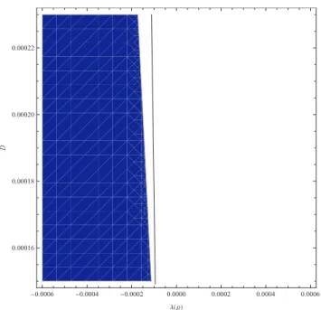
these parameters on single microbubble are presented in previous sec-tion (SeeFig. 1andFig. 2). Studying the dynamics of N bubble cluster for detecting the stable domain at synchronized state is reduced to the study of a single bubble dynamics (Eq.(18)). At same time, it is found to be directly dependent on distances between them (Eq.(32)). In addi-tion, it provides a variable synchronization condition. The inequality condition shows permissible values of distance between microbubbles, and these values they are in the stability region. Recent studies have demonstrated that when inter-bubble distances in a cluster are small, the effects of coupling between the bubbles can be significant[70]. By varying the pressure, permissible value for synchronization with respect to the distances is restricted in the region100⩽D(μm)⩽250. Critical value of pressure for synchronization is founded as (λPac∼ −0.0002)(See Fig. 3).Fig. 4depicts, if λf x( )i is a function of driving frequency, then the
permissible value for synchronization with respect to the distances is
⩽D ⩽
160 (μm) 200. Bubbles are in the stability region when the fre-quency varies in the range500⩽ν MHz( )⩽2000. Frequency could be
defined at the specified value (λ f( )∼ −0.0001) as a limit for synchro-nization, which is determined by a tangent inFig. 4. As lifetimes or sizes of bubbles are different and the distribution of cavitation bubbles is inhomogeneous, the description of the motion of bubbles is very complicated. Future work could be concentrated on this function.
6. Conclusion
This paper explained the dynamics driven interaction between the cluster of chaotic oscillators on a network by using the techniques of coupled maps. Here, in this technique, we employed association scheme and the Bose-Mesner algebra in order to calculate the stability of N-oscillators in a cluster at complete synchronization state. Moreover, taking the microbubble-microbubble interaction as an example we have shown that synchronization condition of N-microbubbles in a regular chaotic networks composed of identical elements with symmetric cou-pling strength can be considered as adjacency matrices. On the other hand, several mathematical models, identify bubbles oscillations in a cluster, such as linear theory[71,72]or self-consistent oscillator model [73,74]. When the number of bubbles in a cluster is increased, a sig-nificant error between experimental and theoretical results appear. In the previous studies[75], the applied procedure can facilitate the un-derstanding of cluster formation from the ultrasound echoes and the stable behavior of UCAs network at synchronous mode. When single UCAs in an ultrasonic field demonstrate chaotic behavior λ>0, we perceive that the acceptable bounds on stable synchronous mode be-come smaller than that in the stable or quasi-periodic case. The dis-tances between interacting UCA clusters mainly acquire significance in their synchronization states, which shows that the influence of coupling between microbubbles is always significant, or at least are no longer negligible[20]. In general, our method can be used for studying the behavior of cluster by adding time-delays to the coupled-oscillator proposed in[16,17].
Acknowledgement
Author M.Y would like to thanks Deepak Kumar Singh for insightful Fig. 3. Stability region of three microbubbles: Variation of distances between of
Fig. 4. Stability region of three microbubbles: Variation of distances between of micro-bubbles respect to single UCA Lyapunov exponent when λf xi( )is a function of driving
References
[1] A.L. Klibanov, Invest. Radiol. 41 (2006) 354. [2] K. Hynynen, Delivery Rev. 60 (2008) 1209. [3] L. Rayleigh, Philos. Mag. 34 (1917) 94. [4] M.S. Plesset, J. Appl. Mech 16 (1949) 227.
[5] M.S. Plesset, A. Prosperetti, Annu. Rev. Fluid Mech. 9 (1977) 145. [6] B.C. Eatock, R.Y. Nishi, G.W. Johnston, J. Acoust. Soc. Am. 77 (1985) 1692. [7] B. Noltingk, E.O. Neppiras, Proc. Phys. Soc. Sec. B 63 (1950) 674. [8] J.B. Keller, M. Miksis, J. Acoust. Soc. Am. 68 (1980) 628.
[9] N. deJong, R. Cornet, C.T. Lancee, Simulations, Ultrasonics 32 (1994) 447. [10] C.C. Church, J. Acoust. Soc. Am. 97 (1995) 1510.
[11] H. Takahira, T. Akamatusu, S. Fukikawa, JSME Int. J. Ser. B 37 (1994) 297. [12] A. Doinikov, J. Acoust. Soc. Am. 116 (2004) 821.
[13] A. Prosperetti, A. Lezzi, J. Fluid Mech. 168 (1986) 457. [14] C.A. Macdonald, J. Gomatam, Proc. IMechE 220 (2006) 333.
[15] K. Yasui, T. Lee, A. Tuziuti, T. Kozuka Towata, Y. Iida, J. Acoust. Soc. Am. 126 (2009) 973.
[16] A.A. Doinikov, R. Manasseh, A. Ooi, J. Acoust. Soc. Am. 117 (2005) 47. [17] A. Ooi, A. Nikolovska, R. Manasseh, J. Acoust. Soc. Am. 124 (2008) 815. [18] U. Parlitz, C. Englisch, C. Scheffczyk, W. Lauterborn, J. Acoust. Soc. Am. 88 (1990)
1061.
[19] S. Behnia, M. Yahyavi, F. Mobadersani, Appl. Math. Comput. 245 (2014) 404. [20] F. Dzaharudin, S.A. Suslov, R. Manasseh, A. Ooi, J. Acoust. Soc. Am. 134 (2013)
3425.
[21] S. Behnia, H. Zahir, M. Yahyavi, A. Barzegar, F. Mobadersani, Nonlinear Dyn. 72 (2013) 561.
[22] K. Kaneko, Progr. Theor. Phys. 72 (1984) 480.
[23] K. Kaneko, Theory and Applications of Coupled Map Lattices Vol. 159 Wiley, New York, 1993.
[24] I. Waller, R. Kapral, Phys. Rev. A 30 (1984) 2047. [25] K. Kaneko, Physica D 37 (1989) 1.
[26] S.I. Tadaki, M. Kikuchi, Y. Sugiyama, S. Yukawa, J. Phys. Soc. Jpn. 67 (7) (1998) 2270.
[27] S.I. Tadaki, M. Kikuchi, Y. Sugiyama, S. Yukawa, J. Phys. Soc. Jpn. 68 (9) (1999) 3110.
[28] S. Yukawa, M. Kikuchi, J. Phys. Soc. Jpn. 64 (1) (1995) 35. [29] K. Shinoda, K. Kaneko, Phys. Rev. Lett. 117 (25) (2016) 254101.
[30] K. Kaneko, I. Tsuda, Chaos and Beyond Vol. 10 Springer, Berlin, 2000 Academic, London.
[31] A.M. Hagerstrom, T.E. Murphy, R. Roy, P. Hövel, I. Omelchenko, E. Schöll, Nat. Phys. 8 (9) (2012) 658.
[32] W. Just, J. Stat. Phys. 79 (1995) 429.
[33] M.C. Ho, Y.C. Hung, I.M. Jiang, Phys. Lett. A 324 (2004) 450. [34] M. Saito, J. Phys. Soc. Jpn. 61 (6) (1992) 1895.
[35] P. Hadley, M.R. Beasley, K. Wiesenfeld, Phys. Rev. B 38 (1988) 8712. [36] W.J. Rappel, Phys. Rev. E 49 (1994) 2750.
[37] R. Albert, A.L. Barabási, Rev. Mod. Phys. 74 (1) (2002) 47.
[38] D.J. Watts, S.H. Strogatz, Nature 393 (6684) (1998) 440. [39] T. Gross, H. Sayama, Adaptive Networks, Springer, 2009. [40] A.E. Motter, C. Zhou, J. Kurths, Phys. Rev. E 71 (1) (2005) 016116. [41] L. Pecora, T. Carroll, Phys. Rev. Lett. 64 (1990) 821.
[42] C.W. Wu, Synchronization in Complex Networks of Nonlinear Dynamical Systems Vol. 76 World Scientific, 2007.
[43] V. Belykh, I. Belykh, M. Hasler, Physica D 195 (2004) 159. [44] F.M. Atay, T. Biyikoglu, Phys. Rev. E 72 (2005) 016217.
[45] I. Belykh, M. Hasler, M. Lauret, H. Nijmeijer, Int. J. Bifurcation Chaos Appl. Sci. Eng. 15 (2005) 3423.
[46] R.C. Bose, K.R. Nair, Sankhya: Indian J. Stat. (1941) 361. [47] R.C. Bose, Pacific J. Math 13 (1963) 389.
[48] R.C. Bose, D.M. Mesner, Ann. Math. Statistics 30 (1959) 21. [49] R.A. Bailey, Association Schemes: Designed Experiments, Algebra and
Combinatorics, Cambridge University Press, 2004.
[50] A.E. Brouwer, W.H. Haemers, Spectra of Graphs, Springer, 2011. [51] C. Godsil, G. Royle, Algebraic graph theory, Springer, New York, 2001. [52] J.L. Gross, J. Yellen, Handbook of Graph Theory, CRC Press, 2004. [53] R.C. Bose, T. Shimamoto, J. Am. Stat. Assoc. 47 (1952) 151.
[54] M. Marcus, Introduction to Linear Algebra, Courier Dover Publications, 1988. [55] M. Burrow, Representation Theory of Finite Groups, Courier Dover Publications,
2013.
[56] E. Bannai, T. Ito, Algebraic Combinatorics. I. Association Schemes, Menlo Park california, 1984.
[57] C. Godsil, Algebraic Combinatorics, CRC Press, 1993. [58] N. Gupte, A. Sharma, G.R. Pradhan, Phys. A 318 (2003) 85.
[59] D.L. Isaacson, R.W. Madsen, Markov Chains: Theory and Applications, RE Krieger Publishing Company, 1985.
[60] E. Seneta, Non-negative Matrices and Markov Chains, Springer, 2006. [61] S. Behnia, M. Yahyavi, J. Phys. Soc. Jpn. 81 (12) (2012) 124008.
[62] K. Morgan, J. Allen, P. Dayton, J. Chomas, A. Klibanov, K. Ferrara, IEEE Ultrason. Ferroelectr. Freq. Control 47 (2000) 1494.
[63] K. Yasui, Y. Iida, T. Tuziuti, T. Kozuka, A. Towata, Phys. Rev. E 77 (2008) 016609. [64] K. Yasui, T. Tuziuti, J. Lee, T. Kozuka, A. Towata, Y. Iida, Ultrason. Sonochem. 17
(2010) 460.
[65] H. Takahira, S. Yamane, T. Akamatsu, J.S.M.E. Int, J. Ser. B 38 (1995) 432. [66] R. Mettin, I. Akhatov, U. Parlitz, CD. Ohl, W. Lauterborn, Phys. Rev. E 56 (1997)
2924.
[67] T. Leighton, The Acoustic Bubble, Academic, London, 1994. [68] E. Stride, M.X. Tang, R. Eckersley, Appl. Acoust. 70 (2009) 1352. [69] J. Jimenez-Fernández, Ultrasonics 52 (2012) 784.
[70] R. Manasseh, A. Nikolovska, A. Ooi, S. Yoshida, J. Sound Vibr. 278 (2004) 807. [71] M. Ida, Phys. Lett. A 297 (3) (2002) 210.
[72] D. Zhang, A. Prosperetti, Int. J. Multiphase Flow 23 (3) (1997) 425. [73] C. Feuillade, J. Acoust. Soc. Am. 98 (2) (1995) 1178.
[74] Z. Ye, C. Feuillade, J. Acoust. Soc. Am. 102 (2) (1997) 798. [75] W. Cheng-Hui, C. Jian-Chun, Chin. Phys. B 22 (1) (2013) 014304.