Full Terms & Conditions of access and use can be found at
http://www.tandfonline.com/action/journalInformation?journalCode=uiie21
ISSN: 0740-817X (Print) 1545-8830 (Online) Journal homepage: http://www.tandfonline.com/loi/uiie20
An efficient algorithm for the single machine total
tardiness problem
BARBAROS Ç. TANSEL , BAHAR Y. KARA & IHSAN SABUNCUOGLU
To cite this article: BARBAROS Ç. TANSEL , BAHAR Y. KARA & IHSAN SABUNCUOGLU (2001) An efficient algorithm for the single machine total tardiness problem, IIE Transactions, 33:8, 661-674, DOI: 10.1080/07408170108936862
To link to this article: https://doi.org/10.1080/07408170108936862
Published online: 27 Apr 2007.
Submit your article to this journal
Article views: 52
An efficient algorithm for the single machine total tardiness
problem
BARBAROS
c.
TANSEL, BAHAR Y. KARA and IHSAN SABUNCUOGLUDepartment of Industrial Engineering, Bilkent University, Bilkent 06533, Ankara, Turkey E-mail: [email protected]@bilkent.edu.trorsahun@bilkell/.edu.tr
Received November 1999 and accepted November 2000
This paper presents an exact algorithm for the single machine total tardiness problem
(1//
L
T;). We present a new synthesis of various results from the literature which leads to a compact and concise representation of job precedences, a simple optimality check, new decomposition theory, a new lower bound, and a check for presolved subproblems. These are integrated through the use of an equivalence concept that permits a continuous reformation of the data to permit early detection of optimality at the nodes of an enumeration tree. The overall effect is a significant reduction in the size of the search tree, CPU times, and storage requirements. The algorithm is capable of handling much larger problems (e.g., 500 jobs) than its predecessors in the literature (:s;150).In addition, a simple modification of the algorithm gives a new heuristic which significantly outperforms the best known heuristics in the literature.I. Introduction
In this paper, we present an exact algorithm that signifi-cantly advances the computational state-of-the-art on the single machine total tardiness scheduling problem, 1//
L:=
T;. In this problem, n jobs with known processingtimes and due dates must be sequenced on a single con-tinuously available machine.Ifa job is completed after its due date, it is considered tardy, and is charged a penalty equal to its completion time minus its due date. The object is to find a sequence that minimizes the total tar-diness. The weighted version of the problem is strongly NP-hard (Lenstra et al., 1977). The version with unit weights which we study is NP-hard in the ordinary sense (Ou and Leung, 1990). A pseudo-polynomial time dy-namic programming algorithm is available (Lawler, 1977), whose time bound is0(n4L:=i Pi) or
0(n5max
p;),
j
where Pi is the processing time of jobj andn the number
of jobs. The method relies on a decomposition theorem proved by Lawler (1977), and refined and strengthened by Potts and van Wassenhove (1982, 1987).
1//
L:=
T; was initially introduced by McNaughton (l959) and the first thorough study done by Emmons (1969), who proves dominance theorems that must be satisfied by at least one optimal schedule. These theorems are later generalized to non-decreasing cost functions (Rinnooy Kan et al., 1975). Exact methods rely either on0740-817X © 2001 "lIE"
branch and bound (Schwimer, 1972; Rinnooy Kanet al.,
1975; Fisher, 1976; Picard and Queyranne, 1978; Sen
et al., 1983; Potts and van Wassenhove, 1985; Sen and Borah, 1991; Szwarc and Mukhopadhyay, 1996) or on dynamic programming (Srinivasan, 1971; Lawler, 1977; Schrage and Baker, 1978; Potts and van Wassenhove, 1982, 1987).
Even though this problem has been around for more than 30 years, relatively little progress seems to have been made in developing effective computational procedures for exact solutions. Early algorithms (e.g., Fisher, 1976) were able to solve problems with about 50 jobs. The dynamic programming-based algorithm of Potts and van Wassenhove (1982) is able to solve problems with 100 jobs and the branch and bound algorithm of Szwarc and
Mukhopadhyay (1996) problems with 150 jobs. An im-portant bottleneck in handling larger-sized problems is the core storage requirement (Potts and van Wassenhove, 1982). The dynamic programming algorithms, developed for this problem require 0(2") storage in the worst case, even though efficient bookkeeping leads to reduced stor-age in most implementations. Branch and bound algo-rithms that use job precedences (Emmons, 1969) at every subproblem requires 0(n2) storage per subproblem, For a
depth-first search that implements cycle prevention rules (needed for consistent application of Emmons' theorems) this amounts to a total core storage of0(n3
) if one keeps an 0(n2) precedence record at every level of the search tree. In contrast, the algorithm that we propose requires
2. Basic results
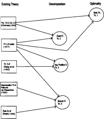
Fig.1. The relationship of the proposed theory to the existing
theory.
OplimaIity ExistingTheory
Theorem 1 of Emmons (1969). For a pair of jobs j and k
with j
<
k,if
a set Bkofjobs isknown 10precede job k in some optimal sequence andif
d, ~ max{p(Bk)+
pi,dk}, then there exists an optimal sequence in which all jobs in BkU{j}
precede job k. Rd&5clt SzwlIt(1996) Th.1dl..8illlr (1977) Th.5ot' CIB1g.'8/
1 ' ' < 4 -(1995)Ths.1&2,Car.l---~
dElnrms(1969algorithm. Additionally, we briefly discuss time and storage requirements of the algorithm. In Section 7, we present and discuss the computational results. In Section 8, we present two new heuristics and discuss their com-putational performance. The paper ends with concluding remarks in Section 9.
In this section, we present the existing theory that we use in our algorithmic design, namely the first and second theorems of Emmons (1969) and the theorem due to Lawler (1977).
Let J
=
{I, ...,n} and let Pj, d, denote, respectively,the processing time and due date of job j. For any
se-quence S of job indices, let Cj(S) be the completion time
of job j in sequence S. The total tardiness associated with
S is T(S)
=
LjEJmax(O, Cj(S) - dj). The problem is tofind a sequence S* such that T(S*) ~ T(S) \;fS. For any
subset KofJ, letp(K)
=
LjEKPj-core storage requirement of0(n2) .Hence, computational
difficulties related to limited storage begin to arise at
much largernin our branch and bound algorithm than in
the existing algorithms. In addition, an efficient and simplified way of handling the data allows us to auto-matically enforce cycle prevention which is a computa-tionally expensive but unavoidable task for the existing methods.
With these features, the proposed algorithm is capable of handling much larger problems (e.g., 500 jobs) than its predecessors in the literature. The CPU times based on 2800 test problems indicate that problems with 500 jobs can be solved to optimality with a 87.5% success rate while those with 400 and 300 jobs can be solved optimally with a 95 and 100% success rate, respectively. The test sets are generated using the method of Fisher (1976), which has been used in the literature to evaluate the previous state-of-the-art algorithms (e.g., Potts and
van Wassenhove, 1982; Szwarc and Mukhopadhyay,
1996). The algorithm and the test sets are available in
the web site http :\\www.bi/kent.edu.tr\~bkara.
The proposed algorithm is a depth-first branch and bound algorithm with three major phases: f3-sequence construction and f3-test, decompositions, and fathoming tests. The f3-sequence constructed in the first phase of the algorithm is a critically important sequence which often solves the problem optimally. The f3-test is a simple check for optimality of the f3-sequence. If the test is passed the optimal sequence is at hand. Otherwise, the algorithm continues with the decomposition phase that utilizes three different decomposition rules: exact de-composition, key position dede-composition, and branch decomposition. Fathoming tests are done by means of a lower bound or by checking if the current job popula-tion matches one of the earlier job populapopula-tions that have already been solved optimally (found-solved). This basic structure is repeated at each node of the search tree.
The proposed algorithm is justified on the basis of four
theorems. Theorem I
(fJ-
Theorem) gives sufficientcon-ditions for optimality. This theorem is proved on the basis of Emmons (1969) and Lawler (1977). The exact decomposition (Theorem 2) is obtained from Emmons' first and second theorems extended via Lawler (1977). The key position decomposition (Theorem 3) and the branch decomposition (Theorem 4) are direct extensions
of the decomposition theorems of Changet al.(1995) and
also those of Potts and van Wassenhove (1982) via Lawler (1977). The relationship of the proposed theory to the existing theory is summarized in Fig. I.
The paper is organized as follows. In Section 2, we provide the basic results from the literature that we use in
our algorithmic design. In Section 3, we prove the
13-optimality. In Section 4, we give an efficient method to construct the fJ-sequence. In Section 5, we give three de-composition theorems. In Section 6, we give the proposed
Theorem 2 of Emmons (1969). For a pair of jobs j and k
with j
<
k,if
sets B, and Ak ofjobs are known to precede and succeed job k, respectively, in some optimal sequence, dj>
max {P(Bk)+
p«. dd, and d,+
Pj?
p(J - Ad, then there exists an optimal sequence in which all jobs inAkU{j} succeed job k.
We refer to B, and Aj as the predecessor and successor sets of jobj, respectively, if jobs in B, are known to precede and jobs inAj are known to succeed jobj in at least one
optimal sequence. In addition, we let E,
=
p(Bj)+
Pj, Lj=
p(J - Aj) and refer to these as the earliest and latestcompletion times of jobj, respectively.
The following corollary to Theorem 2 (Emmons, 1969) gives sufficient conditions for optimality of the Earliest Due Date (EDD) sequence.
Corollary 2.2 of Emmons (1969). The EDD sequence is
optimal if it results in waiting times ffj:S d, (i.e.,
CiEDD)-pj
:s
dj) for all jobs j.The next theorem states that the due dates can be mod-ified in appropriate ranges without losing optimality. Theorem 1 of Lawler (1977). Let S* be any sequence which
is optimal with respect to the given due dates d, ... , dnand
let Cj(S*) be the completion time ofjob j for this sequence. Let d; be chosen such that min(dj, Cj(S*»
:s
d;:s
max(dj, Cj(S*». Then any sequence Sf which is optimal with respect to the due dates d;, ... ,d~ is also optimal with respect to the due dates d., ... , d; (but not conversely).3. fJ-Optimality
Assume the jobs inJ are indexed in non-decreasing order of processing times with ties broken by non-decreasing order of due dates. Given an instance of the problem with due dates dj , suppose we have applied (without creating
cycles) Theorems I and 2 of Emmons (1969) and obtained predecessor sets Bj. Let ~j = p(Bj)
+
PjandP
j = max(dj, p(Bj )+
Pj) Vj. Clearly ~j is a lower bound for thecom-pletion time of jobj in any optimal sequence that satisfies the precedence relations with respect to the setsBj .Define
the p-sequence to be the sequence such that the jobs are ordered in non-decreasing order of their
P
j values with tied ones ordered in increasing order of job indices. Let.r
= {j EJ :3 i>
j such thatP
j>
PJ.
Theorem 1 (fJ-theorem). The p-sequence is optimal
if
P
j?
p(Fj) Vj E.r
where Fj is the set ofjobs that precede job j in the p-sequence.Proof. We first prove that the p-sequence is optimal for the problem with due dates
d;
=
P
j , then prove that it isalso optimal for the original problem. Let j E J. If
j EJ*, then the assumption of the theorem gives
P
j?
p(Fj)=
ffj (where ffj is the waiting time of job j in the p-sequence). If j!f;J*, then Fj=
{i: pi:S Pj andPi
:s
P
j } (due to the indexing convention). Itfollows fromTheorem I of Emmons (1969) that every jobiinF,is also in
s;
Hence,P
j?
~j=
p(Fj)+
Pj>
p(Fj)=
ffj. We have shown thatP
j ? ffj Vj EJ. Corollary 2.2 (Emmons, 1969) implies that the p-sequence is optimal for the problem with due datesP
j .Observe that the interval [dj, max(dj,~)] is a subin-terval of the insubin-terval [min(dj, Cj(S*», max(dj, Cj(S*»]
where S* is any optimal sequence that satisfies the pre-cedence relations relative to the sets Bj .Sinced;
=
P
j is inthis interval, the p-sequence is optimal for the problem with due dates d, as a result of Theorem I of Lawler
(1977). •
The proof of Theorem I provides an important idea which we term the idea of equivalence. By observing that the new due dates
d;
=
P
j are in the intervals[dj ,
max(dj,~)], this idea permits every theoretical statement that is valid for the original problem to be re-stated in terms of the data of the new problem while ensuring that the conclusions obtained from such statements remain valid not only for the new problem but also for the original problem. The idea of equivalence is also used in the proofs of Theorems 2, 3, and 4 in the sequel, thereby greatly increasing the utility of the existing theory by appropriately modifying the due dates during the branch and bound algorithm. Even though the root of the equivalence idea lies in Theorem 1 of Lawler (1977), it should be noted that Lawler's theorem alone does not provide a way of creating the modified problem because it requires knowing an optimal sequence. On the other hand, replacing Cj(S*) with~j circumvents this difficulty in a simple but strong way by eliminating the need to know an optimal sequence.
4. Sequence construction
Theorem I gives sufficient conditions for optimality of the p-sequence which is nothing but the EDD sequence with respect to modified due dates obtained through the use of the dominance theorems of Emmons (1969). In this sec-tion, we present a method of constructing this sequence in an extremely efficient way. If the p-sequence satisfies the sufficient conditions of Theorem I, an optimum is at hand. Otherwise, the problem is decomposed to obtain new subproblems each of which goes through the opti-mality test again with respect to their own p-sequences.
Let !Xj = max(pj, dj) Vj. Sequence the jobs in non-de-creasing order of their !Xj values with tied jobs sequenced in increasing order of their indices. The tie breaker defines the resulting sequence uniquely. We call this sequence the
Duedalc
PorthC~iDOfmjob10
LEFT-EXP
AND cxpmItoDfmjob(0 Third~r.-jab10 57 63 66 73 17 82 I"rocea lime 29 43 44 10, . . . f - - - -...
Step 1. Select any jobkwhich is not selected yet (if none left, stop).
Step 2. Compute p(LDk).
Step 3. If p(LDk)
+
Pk>
th,
then increasefi
k top(LDk)
+
pi, redefine LDk with respect to the new point (Pk,f3r
eW) and return to Step 2). Otherwise,add jobk to the list of seleeted jobs and return to Step 1).
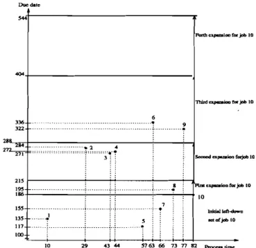
Fig. 2. lllustration of procedure LEFT-EXPAND for job 10.
Example I the procedure is illustrated in Fig. 2 for
k
=
10. Initially, 1310=
alO=
186 and LDIO= {I,5, 7}.With p(LDIO)
+
PIO = (10+
57+
66)+
82 = 215, Step 2updates 1310to 215 and LDIOnow includes job 8 in
addi-tion to 1,5,7. The vertical arrow that originates at job 10's point in the figure indicates this expansion. The procedure continues with the second, third, and forth expansions as shown by the vertical arrows. The final /310 is 544 and LDIOis
{1,
2,3,4,5,6,7,8, 9}.Let
fJ
=
(/31" .. ,f3n) be a vector of/3j values of jobs at any time during the operation of algorithm LEFT-EX-PAND. Redefine LDj, LVj,RVj,RDj,Dj, Uj, and J* with respect to the points (PI, fil), ... , (Pn, /3n)'The fJ-test can be conducted at any time during the algorithm LEFT-EXPAND. A positive answer is con-clusive (optimum at hand) while a negative answer signals the need to further increase the f3j values (especially those that failed in the test). In case of failure of the optimality test, we can use the information available in the right-down sets to further increase the f3j values based on
Theorem 2 of Emmons. For a fixed jobj, if we choose a
Property 1 gives an easy way to build the predecessor sets of all jobs. The O(n2) procedure below accomplishes this
by successively expanding left-down sets. This procedure defines the fJ-sequence recursively. We begin the proce-dure with
fi
j = aj Vj (or with the most recentfi
j valuesobtained from the procedure RIGHT-EXPAND which is explained later).
Property l. There is an opl imal sequence such thaI LDj is a predecessor set ofjob j and RVj is a successor set ofjob j. (Modified Due Date) (Baker and Bertrand, 1982) which replaces a job's due date by the current time t plus that job's processing time whenever d,
<
t+
Pj gives the ajvalues ift= O. However, we use the a-sequence as a seed to begin the construction of the {i-sequence, rather than as a heuristic rule. Observe that any optimal solution to the problem with due dates aj is also an optimal solution for the problem with the original due dates d.. This fol-lows from the fact that Pj
>
d, implies jobj will be tardy regardless of where it is placed in the sequence. Hence, shifting its due dates to Pi simply changes the tardiness of job j by a constant amount (see also Tansel andSab-uncuoglu (1997) for additional discussion).
For fixed
i-
partition J - {j} into sets LDj=
{i
EJ :i
<
j and ai::; aj}, LVj=
{i EJ: i<
j and «,>
aj},RDj=
{i EJ :i>
j and ai<
aj}, and RVj=
{i EJ :i>
jand a,2:aj}' We call LDj(RDJl the left-down (right-down)
set and LVj(RVj) the left-up (right-up) set of job j. The terminology is motivated by the fact that if we plot the points (PI,al),' .. , (Pn, an) in the plane and pass a
hori-zontal and a vertical line through the fixed point (pj, aJl, the plane is divided into four quadrants at (pj, aJl each of which contains one of the above-mentioned sets. Note that jobs whose points fall on the horizontal or the ver-tical line through the point (Pj, aj) belong either to the left-down set or the right-up set of job j depending on their indices. Note also that if (Pi, ai)
=
(Ph aj), then iis inLDj if i
<
j and i is in RVj if i>
j. Let D,=
LDj U RDjand U, = LVj U RVj. Call D, the down-set and U, the
up-set of jobj.
The final fi-sequence is constructed from the a-se-quence by means of successive transformations of due dates. Observe that if we take the initial fi-sequence to be the a-sequence, then the setF,in Theorem 1 is the same as D, and J* = {j EJ :RDj
=!'
0}. We refer to the checkingof sufficient conditions
fi
j 2:p(Dj ) Vj EJ* as the fi-test.We initially apply this test to the a-sequence. If the test fails, the data transformation is initiated and continued until either the fi-test is passed or the transformation is no longer possible. This transformation of the problem into a new form which is more easily solvable than the initial form is one of the features that distinguishes our algo-rithm from the existing algoalgo-rithms.
The following property is a direct consequence of Theorem I of Emmons (1969):
job k in the most recent right-down set of jobj, all con-ditions of Emmons' second theorem except possibly the last one are automatically satisfied. That is, if we take
Bk
=
LDk,A k=
RUb and regardP
j and 13k to be the newdue dates, then the only remaining condition that needs to be checked is the inequality
f3
j+
Pj :::: p(J - RUk) (thecondition
f3
j>
max(p(Bkl+
Pk, dk) in Theorem 2 ofEm-mons(1969) is automatically satisfied by all jobsk inRDj
since
P
j>
13k for such jobs due to the definition ofRDj ).Whenever this inequality is satisfied, job k qualifies as a
predecessor to job
i-
Such jobs in the right-down set of a given job can be used to further increase the I'lj value ofthat job. This is done by the following 0(n2) procedure, RIGHT-EXPAND.
RIGHT-EXPAND
Step O. Let B, = LDj and Aj = RUj 'if) where LDj, RUj
are the left-down and right-up sets corresponding to either
f3
j=
!Xj'if)or the most recent values off3l,f32, ... ,f3n
obtained from LEFT-EXPAND. Let Ej=
p(Bj)+
Pj and L,=
p(J - AJl 'ifj. Set )=n+l.Step 1. Set)<-) - I. If)
=
0 stop, else go to Step 2.Step 2. Identify all jobs kERDj (defined by the most
recent
f3
j values) which are not in B, and which satisfy the inequalityf3
j+
Pj :::: Lk. Let R be theset of jobs so identified. IfRis null, go to Step I; else go to Step 3.
Step 3. ReplaceB,byB)UR and increaseE,bypeR). For
eachk in R, replace Ak byAkU {j}and decrease
Lk by Pj' If Enew
>
f3
j , increasef3
j to E)new, and) .
return to Step 2. Otherwise return to Step I. Consider the following example:
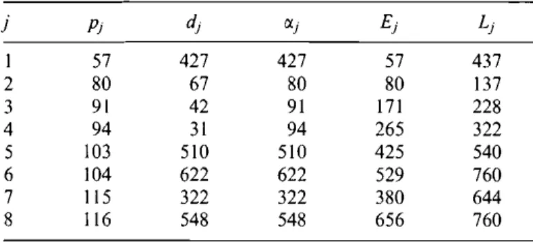
Example2. TheE,andL, values in Table I are computed with respect to the LD; and RDj sets defined by the r:t.j
values. For example,'E4= p(LD4)
+
P4 where LD4 ={2, 3}. For)
=
8,7, Step 2 outputs empty RDj .Continu-ing with)
=
6, Step 2 gives RD6=
{7, 8} and R=
P}.Table l. The data for Example 2
j Pj d j rxj
s,
L j 1 57 427 427 57 437 2 80 67 80 80 137 3 91 42 91 171 228 4 94 31 94 265 322 5 103 510 510 425 540 6 104 622 622 529 760 7 115 322 322 380 644 8 116 548 548 656 760Hence, Step 3 givesB6=LD6UR={1,2,3,4,5,7},
in-creases E6 to 644, updates A7 to RU7 U {6}
=
{8, 6}, de-creases L7 to 540, and increases 136 to 644. Returning to Step 2, with)=
6 again, the execution of Steps 2 and 3 yield no change for this job, so the algorithm returns to Step I and continues with)=
5. Processing job 5 through two cycles of Steps 2 and 3, we obtainB5= {I, 2, 3,4, 7},E5
=
540,A7=
{8, 6, 5},L7=
437, and 135=
540. Con-tinuing in like manner with emptyRDj sets for)=
4,3,2and with two passes of Steps2 and 3 for)
=
1, we obtain the final f3-sequence (2,3,4,7, 1,5,6,8) with correspond-ingP
j values of (80, 171,265,380,437,540,644,656).We experimented with three strategies for constructing the f3-sequence which we call LEFT, LEFT-RIGHT, and FULL. LEFT uses only EXPAND while LEFT-RIGHT first uses LEFT-EXPAND, then switches to RIGHT-EXPAND, then executes LEFT-EXPAND one more time and stops. FULL uses LEFT-EXPAND and RIGHT-EXPAND repeatedly, one after the other, until no further updating occurs in the
f3
j values. The number of nodes of the enumeration tree generated by LEFT exceeds in general those generated by LEFT-RIGHT which usually marginally exceeds those generated by FULL. Based on our computational tests, we note how-ever that, in terms of average CPU times, LEFT generally outperforms both LEFT-RIGHT and FULL except for the most difficult classes of instances. A more detailed discussion of the efficiency issues is given in Section 6.5. Decomposition
In this section we give three decomposition theorems: exact, key position, and branch decomposition. All of these decompositions try to identify a position in the se-quence to split the problem into subproblems. However, there is a major difference between branch decomposition and the other two. Whereas branch decomposition can only identify a set of candidate positions for splitting the problem, the other two find a specific position for de-composition. Branch decomposition leads to different branches from a given node in a branch and bound pro-cedure and to different states in a dynamic programming procedure. Either way, branch decomposition typically leads to an exponential number of subproblems. In con-trast, exact and key position decompositions do not lead to any branching. Hence, the major strength of exact and key position decompositions is their ability to continue with a single branch (or a single state in dynamic pro-gramming), but their major weakness is that there is no guarantee that such a decomposition may exist. Conse-quently, the latter two types of decompositions do not have the ability to lead to a branch and bound or dynamic programming algorithm. However, if they are combined with branch decomposition, the outcome is a faster branch and bound or dynamic programming procedure.
In the proposed algorithm, we use exact decomposition whenever the (J-test fails. If no job qualifies for exact decomposition, we continue with key position decompo-sition which is an enhanced version of Theorem 5 of Chang et al. (1995). If this decomposition also fails, we continue with branch decomposition which is an en-hanced version of the decomposition proposed by Potts and van Wassenhove (1987). The lalter two decomposi-tion theorems are enhanced in that the {Jj values are used in these theorems instead of the initial due dates, thereby permitting repeated use of these theorems with continu-ally modified data. Note that the original decomposition of Lawler (1977) is also in the category of branch composition. In fact, Potts and van Wassenhove's de-composition strengthens Lawler's by eliminating certain alternative decomposition positions.
The exact decomposition theorem looks for a jobqthat qualifies for decomposition and assigns it to a specific position in the sequence which splits the problem into two subproblems corresponding to the down-set and up-set of job q. The theorem uses the information that is available at the end of the construction of the {J-sequence. This information includes the final sets, LD j, LUj, RDj, RUj, as well as the final values of the latest times LI, ... .L; (If LEFT is used, the L/s are taken to be p(J) - p(RUj)
where the RU/s are the final right-up sets at the end of LEFT-EXPAND). Note that the time complexity of searching for a job q that qualifies for exact decomposi-tion is0(n2
) .
Theorem 2(Exact decomposition). Let q EJ. If (i) either RDq=
0
or pq+
{Jq ::::i,ViERDq and (ii) either LUq=
0
or Pj+
{Jj :::: LqVj E LUq,then there is all optimal sequence such that all jobs in Dq precede q and all jobs in Uq succeed q. This implies that the problem decomposes in the form (Dq ,q, Uq ) where the
subproblems corresponding to the sets Dqand Uqare solved
independently. The jobs in Uq have a ready time of
p(Dq )
+
pq.sequence that obeys the so far obtained precedence rela-tions, then {;.j
:S:
Cj(S*)V j so that (Jjare in the intervals[min(dj, Cj(S*)), max(dj, Cj(S*))]. Theorem I of Lawler
(1977) implies that (SI, q, S2) is an optimal sequence with
respect to due datesd., ... ,d., •
Given the earliest times EI , • . • ,En and the latest times
LI , ..•.L; during or at the end of the construction of the
{J-sequence, ifE,
=
L, for somej then the problem clearly decomposes in the form (Dj,j, Uj) which is the kind of block decomposition given by Szwarc andMukhopad-hyay (1996). In this case, it is straightforward to show
that conditions (i) and (ii) of Theorem 2 are satisfied. However, Theorem 2may yield a decomposition even if
E,
<
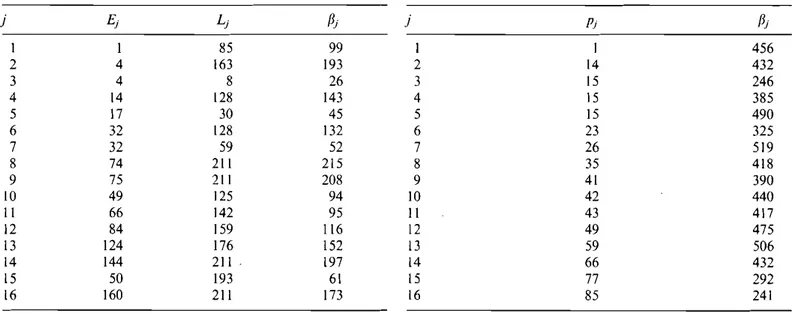
Lj Vj. Example 3illustrates this.Example3. The data for this example are given in Table2. TakingB,
=
LDj,Aj=
RUj and{Jj=
max(Ej, dJl, we have the results listed in Table 3. Even though E,<
L, Vj, there is a decomposition at job 7since RD7=
0
and {JI+
PI
=
99+
I > L7=
59, {J2+
P2=
193+
3> L7, {J4+
P4=
143
+
9> L7, {J6+
P6=
132+
14> L7. Thus, jobs D7=
{3,5} and U7 = {1,2,4,6,8,9, 10,II, 12, 13, 14, 15, 16}
can be sequenced independently.
Next we give the key position decomposition theorem. Theorem 3 (Key position decomposition). Let Sp
=
(11], ... ,
[n]) be the (J-sequence and assume job n is in po-sitionk in Sp. Let Sp(i) be the sequence obtainedfrom Sp by moving job n from position k to position i and let T(Sp(i)) be the total tardiness of Sp(i) computed with respect to the due dates {JI"" ,(In' Define the key position index h to be the smallest index such thatT(Sp(h))
=
min T(Sp(i)fk5:i'.5:n
Table 2. The datafor Example3
j
Proof. Consider the problem with modified due dates {JI,' .. ,{JI/' For this problem it can be shown, via Theorem 2 of Emmons (1969) that (i) in the theorem implies that
RDqis a predecessor set ofqwhile (ii) implies thatLUqis a
successor set of q. Property I implies that LDq is also a predecessor set of q and RUq is also a successor set of q.
Hence, Dqis a predecessor set and Uqis a successor set for
jobq for the problem with due dates {JI'" . ,{In, i.e., there
exists a sequence S = (SI,q,S2) which is optimal with respect to due dates {JI," .,{In such that Sl is a
permu-tation ofDqand S2 is a permutation ofUq .Consider now the original problem with due dates d., .. ..d., If we as-sign{;.j
=
E, where the E/s are the earliest times obtained a t the end of the construction of the {J-sequenee, then the due dates {Jj E [dj, max(dj, {;.j)]' If S* is an optimalI 2 3 4 5 6 7 8 9 10 II 12 13 14
is
i6 I 3 4 9 13 14 15 15 16 17 17 17 17 17 18 18 99 193 26 143 45 132 52 215 208 94 95 116 152 197 61 173If h
<
n, then there is a sequence S=
(SI, S2) which is optimal for the problem with due dates fJ" ... , fJn as well as for the original problem such thatSIis a permutation of the jobs that occupy the first h positions in Sp while S2 is apermutation of the jobs that occupy the last n - hpositions in Sp.
Proof. The theorem is an equivalent statement of Theo-rem 5 of Chang et al. (1995) where the d/s are replaced by the fJj'S and the EDD sequence is replaced by the
fJ-sequence. Hence, the optimality of S
=
(S" S2) for the problem with due dates fJI' ... ,fJnis immediate from the theorem of Chang et al. (1995). The optimality ofS= (SI, S2) for the original problem follows from Law-ler's theorem using again the fact that fJ; E [dj , max(dj,.G:j)] I:;; [min(dj ,Cj(S*)),max(dj, Cj(S*))] where S*
is an optimal sequence that obeys the obtained
prece-dence relations. •
With the above theorem, whenever the key position index
h
<
n, we can split the current job population into two subproblems, one consisting of the jobs in positions 1, ...,h in the fJ-sequence, the other consisting of those in positions h+
I, ... ,n in the fJ-sequence. The ready time of the latter set is redefined to be the sum of the pro-cessing times of the first set. Note that checking for key position decomposition takes 0(n2) time.
Both Theorems 2 and 3 are based on the fJ-sequence. The two theorems differ in two respects:
1. The key position decomposition can be carried out only relative to the longest job whereas the exact decomposition can be carried out relative to any qualifying job q.
2. Key position decomposition decomposes the prob-lem into two sets without specifying the position of
any of the jobs (including the longest job) whereas the exact decomposition specifies the position of the qualifying job q.
Next, we present the branch decomposition. In what follows, we say jobj passes the fJ-test withstrict inequality
if fJj
>
p(Dj ) and with equality if fJj = p(Dj ) . If Dj =0,
take p(Dj )
=
O. Theorem 4 below is an equivalentstate-ment of Potts and van Wassenhove (1987) decomposition where thed/s are replaced by the fJ/s. Lawler's theorem implies that the resulting decomposition for the problem with due dates fJt, ... ,fJn is also valid for the original problem.
Theorem 4 (Branch decomposition). Assume job n is in
positionk in the fJ-sequence. The problem decomposes with jobn in position Ifor someIsatisfying one of the following
conditions:
(i) 1= k and the (k
+
I)st job in the fJ-sequence passes the {i-test with strict inequality.(ii) I E {k
+
I, ... .n - I} and the (I)th job either fails the fJ-test or passes with equality while the (I+
I)st job passes the test with strict inequality.(iii) 1= nand the (n)thjob either fails the test or passes with equality.
The following example illustrates the Branch decompo-sition.
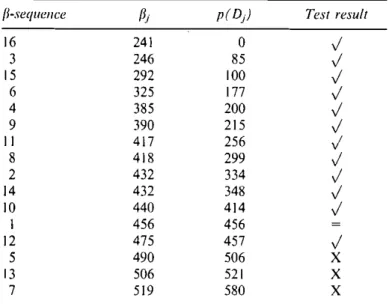
Example4 the data for this example are given in Table 4. The job with the largest processing time is job 16, and it is in the first position of the fJ-sequence, so k
=
I. ThefJ-sequence, together with fJj values, down-set totals of the jobs, and passes and fails of the test are given in Table 5. A ""j" stands for a pass with strict inequality, an "="
sign stands for a pass with equality, and an "X" stands
Table 3. The results for Example3 Table4. The data for Example 4
j Ei Li fJi j Pi fJi I I 85 99 I I 456 2 4 163 193 2 14 432 3 4 8 26 3 15 246 4 14 128 143 4 15 385 5 17 30 45 5 15 490 6 32 128 132 6 23 325 7 32 59 52 7 26 519 8 74 211 215 8 35 418 9 75 211 208 9 41 390 10 49 125 94 10 42 440 11 66 142 95 II 43 417 12 84 159 116 12 49 475 13 124 176 152 13 59 506 14 144 211 197 14 66 432 15 50 193 6\ 15 77 292 16 160 211 173 16 85 241
Table 5. The results for Example 4
{i-sequence (ij p(D) Test result
16 241 0
.;
3 246 85.;
15 292 100.;
6 325 177.;
4 385 200.;
9 390 215.;
II 417 256.;
8 418 299.;
2 432 334.;
14 432 348.;
10 440 414.;
I 456 456 = 12 475 457.;
5 490 506 X 13 506 521 X 7 519 580 Xfor a failure of the test. The test results imply directly that the problem decomposes with job 16 in positions I, 12, and 16.
Szwarc and Mukhopadhyay (1996) give an additional rule that eliminates some of the positions permitted by the decomposition of Potts and van Wassenhove (1987). This rule is adapted to the f3-sequence as follows. The algorithm BETA uses this additional rule in the Branch decomposition.
Rule 5c ( Szwarc and Mukhopadhyay (/996)). Let the
fJ-sequence be [I], ... ,
[n]
and assume jobn
is in positionkin the {i-sequence. Then job n is not in position .1',.I' ~ k, ifthere exists a job i, i E
Uk
+
I]' ... ,[.I' - I]} such thatPII]
+ ... +
Plk-I]+
P[k+I]+ ... +
Pis]+
Pin] :SPi+
d., Rule 5c additionally eliminates position 12 in Example 4 since 372+
85<
PI4+
dl 4=
498.6. The algorithm
The proposed algorithm, which we call BETA, is a depth-first branch and bound algorithm. The algorithm depth-first checks whether the problem on hand is in the list of already solved subproblems (found-solved). If not, the
f3-sequence is constructed and the fJ-test applied. If the test
is passed, then the fJ-sequence is optimal. Otherwise, the algorithm looks for a job that qualifies for exact decomposition. If such a job is found, the problem is decomposed and each subproblem is solved via BETA. Otherwise, the algorithm looks for a position h that qualifies for key position decomposition. If such a position is found, decomposition is applied and the subproblems are solved via BETA. Else, the algorithm continues with branch decomposition. During the
processing of the branches, BETA is called separately for each branch and two fathoming criteria are applied, one based on found-solved, the other one based on a lower bound. An example that illustrates the algorithm is given in the Appendix.
Of the two fathoming criteria,found-solved first checks
at each branch if the subproblem under consideration has already been solved during the processing of some other branch. If the answer is yes, just take the solution, oth-erwise continue with the algorithm in the usual way . Found-solved significantly reduces the number of branches in most instances. As a result, the total CPU time decreases even though additional time is spent per branch for checking the pre-solved problems. The found-solved list contains the most recent k subproblems that have been solved during the algorithm where k
=
1000 in our implementation.The second fathoming criterion is based on a lower bound. For the lower bound computation, we use the
fJ-sequence and define a relaxed problem with new due dates djew
=
max{fJj,p(Dj )} . With the new enlarged duedates, the fJ-test will necessarily pass and the resulting
fJ-sequence will be optimal for the modified problem. Since
dr
w ~ fJj 'ifj, the total tardiness of the fJ-sequence with
respect to the new due dates gives a lower bound. We proceed with the fJ-test only if the lower bound fails to fathom that node.
A few words on simplified bookkeeping and compu-tational efficiency of the algorithm are in order. The bookkeeping is greatly simplified by keeping an n-vector which concisely represents all precedence relations. This n-vector contains the job indices in the same order as they appear in the fJ-sequence (and the associated records
fJj, Ej, Lj,pj, d, 'ifj). From this n-vector, one can easily obtain the setsBj ,Aj and the associated earliest and latest times Ej , Lj . This results in O(n) space for keeping track
of precedence relations which lead to 0(n1) space
re-quirement for a depth-first branch and bound tree, whereas existing methods accomplish the same thing in
0(n3
) space. As for time requirements, the procedures LEFT and LEFT-RIGHT obtain the fJ-sequence (and hence the associated precedence relations) in 0(n2) time, whereas the existing methods require 0(n4) time (0(n2) checking required each time a new relation emerges) for constructing the precedence diagram.
With these considerations, the time and space re-quirements of the existing methods can easily become prohibitive for n
>
200 whereas our way of handling the data allows us to solve much larger problems. The time bounds of the different components of the algorithm BETA are given in Table 6. Computational tests indicate that, on the average, about 80% of the total CPU time per branch is spent on the fJ-sequence computation, about 15% on exact and key position decomposition, and about 5% on branch decomposition, lower bound, and found-solved.Table 6. Time bounds of the phases of BETA
f)-sequence
const rueIion
0(n2) for LEFT or LEFT-RIGHT 0(n4) for FULL Optimality check (f)-test) O(n) Exact decomposition Branch decomposition O(n) Key position decomposition Lower bound computation O(n) Checking for found-solved O(n) 7. Computational results
The performance of the proposed algorithm is measured on a Spare Station Classic with a 60 MHz microSPARC 8-CPU and a 384 GB main memory. The code is written in the C language. The data generation scheme initially proposed by Fisher (1976), which has traditionally been used in the literature since then, is used to test the algo-rithm for different types of instances. These instances of varying degrees of difficulty are generated by means of two factors: tardiness factor, T, and range of due dates, R.
For each problem, first the process times are generated from a uniform distribution with parameters (I, 100). Then the due dates are computed from a uniform distri-bution which depends on p' ==prj) and on Rand T. The due date distribution is uniform over [p'(I - T - Rj2),
p'(1 - T
+
Rj2)]. The values of T and R are selected fromthe sets {0.2, 0.4, 0.6, 0.8} and {0.2, 0.4, 0.6, 0.8, I}, re-spectively. This gives 20 combinations ofR, T factors for
each problem size. We refer to each (R,T)combination as a problem type. The number of jobs n is chosen from
{IOO, 110, 120,130,140,150,160,170,180,190,200,300, 400, 500}. We solve 10 different instances for each setting ofn,R, T giving a total of 200 instances for each choice of
n. The total number of random instances solved is 2800. The time limit to abandon a solution is 80 hours.
A distinctive feature of the proposed algorithm is that it is capable of handling very large populations of jobs whereas this seems to be an impossibility for the existing algorithms in the literature for II
>
200. Even though thehardest instances could not be solved to optimality for
II
=
500. we still have an 87.5% success rate for this size(i.e., 87.5% of the generated instances with 11
=
500 aresolved to optimality).
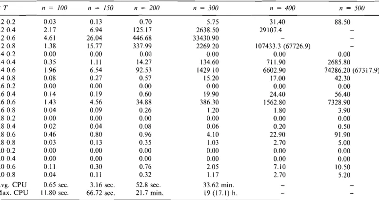
The detailed results are given in Table 7. Each cell in that table represents the average CPU seconds of 10 in-stances for each (R, T) pair and 11.Of the three versions
(LEFT, LEFT-RIGHT, FULL) of the algorithm BETA, the reported numbers except those in parentheses are based on LEFT. The parenthetical numbers are the av-erage CPU seconds for LEFT-RIGHT and are supplied only for those cells where LEFT-RIGHT performed
Table 7. Average CPU seconds for the LEFT version of BETA (numbers in parenthesis are the CPU seconds for LEFT-RIGHT)
RT n = 100 n = 150 11= 200 11= 300 n = 400 II = 50U 0.20.2 0.03 0.13 0.70 5.75 31.40 88.50 0.20.4 2.17 6.94 125.17 2638.50 29107.4 0.20.6 4.61 26.04 446.68 33430.90 0.20.8 1.38 15.77 337.99 2269.20 107433.3 (67726.9) 0.4 0.2 0.00 0.00 0.00 0.00 0.00 0.00 0.4 0.4 0.35 1.11 14.27 134.60 711.90 2685.80 0.4 0.6 1.96 6.54 92.53 1429.10 6602.90 74286.20 (67317.9) 0.4 0.8 0.08 0.27 0.57 15.20 17.00 42.30 0.60.2 0.00 0.00 0.00 0.00 0.00 0.00 0.60.4 0.14 0.19 0.60 19.90 24.40 56.40 0.60.6 1.43 4.56 34.88 386.30 1562.80 7328.90 0.60.8 0.04 0.09 0.26 1.20 1.80 3.90 0.80.2 0.00 0.00 0.00 0.00 0.00 0.00 0.8 0.4 0.02 0.04 0.08 0.06 0.20 0.50 0.8 0.6 0.46 0.80 0.96 4.10 22.90 91.90 0.80.8 0.03 0.13 0.35 1.03 2.70 5.00 1.00.2 0.00 0.00 0.00 0.00 0.00 0.00 1.00.4 0.00 0.00 0.00 0.00 0.00 0.00 1.0 0.6 0.11 0.30 0.76 2.05 7.10 10.50 1.00.8 0.04 0.11 0.32 1.17 2.70 5.20
Avg. CPU 0.65 sec. 3.16 sec. 52.8 sec. 33.62 min.
considerably faster than LEFT. As remarked earlier, even though FU LL gives the best overall performance in terms of the number of branches, its performance in terms of the average CPU seconds is inferior because FULL spends considerably more time per branch to compute the fJ-sequence than either LEFT-RIGHT or LEFT. The number of branches generated by LEFT-RIGHT is generally quite close to those generated by FULL, but LEFT-RIGHT spends much less time per branch than FU LL. Hence, we recommend the use of LEFT-R[GHT for n= 500 for the first four most difficult classes of in-stances corresponding to (R,T) pairs of (0.2,0.6), (0.2,0.8),(0.2,004), (004,0.6), where the trade-off between the number of branches and the CPU time per branch works in favor of the reduced number of branches. The same recommendation is valid for cate-gories (0.2,0.6), (0.2,0.8) for n
=
400. In all the remain-ing cases (i.e., the 16 categories of n=
500, the [8 categories of n=
400, and all 20 categories ofn :S 300), we recommend the use of LEFT as it performs consid-erably better than LEFT-R[GHT in terms of the average CPU time. Note, however, that the maximum CPU time of LEFT-RIGHT is considerably better for largen (n
2:
300) than that of LEFT, e.g., [7.1 hours versus 19 hours for n=
300. The general pattern is that it becomes more advantageous to switch-over to LEFT-RIGHT from LEFT as n increases where the switch-over point is earlier for more difficult classes of instances.As can be seen from Table 7, the average solution time for n= 100 is less than I sec. The average solution times for n= 150,200, and 300 are 3.16 sees, 52.8 sees, and 33.6 minutes, respectively (the averages for n
=
400 and 500 arc not available because not all instances are solved for those sizes). The worst encountered solution times are 11.8 seconds, 1.11 minutes, 21.7 minutes, 17.1 hours forn
=
100, 150,200,300, respectively (more than 80 hours for sizes 400 and 500). Thus, our algorithm handles problems of size 150 very successfully with an average solution time of about 3 seconds while the maximum solution time for 150 job problems is about I minute. 200 job problems are also successfully handled with an aver-age CPU time of less than I minute and a maximum CPU time of about 22 minutes.Table 7 shows that the computation times are highly dependent on the R, T factors. Of the three hard problem types (0.2,0.4), (0.2,0.6), and (0.2,0.8), the most difficult one is the pair (0.2,0.6). For the blank cells in Table 7, the algorithm obtained suboptimal solutions for n= 400, and 500 whose average deviation from optimality is ap-proximately 5%. In all other (R, T) pairs and for all values of n, the algorithm obtained the exact solution for all generated instances.
Observe that five out of 20 (R,T) pairs have a solution time of zero for all n values. Hence, the optimum is im-mediately found in 25% of all instances. These are the problem types corresponding to (R, T) pairs with T= 0.2
with R
=
0.4,0.6,0.8, I and T=
004 with R=
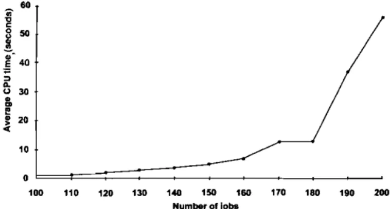
I. The op-timum is immediately found for these problems because either the {1-sequence for the initial job population hap-pens to be the optimum one or a few branches lead to the optimum immediately.Figure 3 shows the average solution times in CPU seconds as a function of n, ranging from 100 to 200. Observe that, up to n
=
130, the solution times are less than 2 seconds. At n=
170 and 180, the solution times are slightly more than lO sec, and at n=
200, it is about 53 seconds. Hence, the slope increases rather slowly, showing almost a linear trend, from n=
100 to 180. Aftern
=
180, exponential behavior begins to take over. Even though our algorithm uses reduced memory (O(n) versus0(n2) in existing algorithms), this exponential behaviour
is partly due to the hard disk and memory requirements. However, our computational experiments up to n
=
500 indicate that, the prohibitive nature of the exponential behavior makes itself felt at much larger n (n>
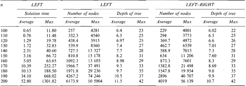
300).Statistics on the performance of the algorithm in terms of solution times, number of nodes and the depth of the tree are given in Table 8 in the range of n
=
100 to 200 with increments of 10. A comparison in terms of relative increase in CPU times indicates that the average solution time of the algorithm of Szwarc and Mukhopadhyay (1996) increases 23.69 times as11increases from 100 to ISO while the average CPU time of BETA increases 4.86 times over the same range. Potts and van Wassenhove (1982) do not report any computational times for this range of n, but their reported results indicate that the CPU time in-creases 35.61 times as n goes from 50 to 100.Szwarc and Mukhopadhyay (1996) report that, for
n
=
ISO, the average number of branches and the average depth of the tree are 9005 and 10.7, respectively. For the algorithm BETA and for n=
150, the average number of nodes is 811(634) and the average depth of the tree is 8.2(7.6) if LEFT(LEFT-RIGHT) is used which indicates that there is a reduction of about 11(14) times in the average number of branches and a reduction 'of about 2.5(3) levels in the average depth of the tree depending on which of LEFT or LEFT-RIGHT is used.60
..
'2too
~ 40 ::>..
(J 30t
!
20 10 o~==::;::=:::==:====~~_
100 110 120 130 140 150 160 170 180 190 200 Number of jobsTable 8. Average and worst case statistics fornvalues ranging from 100 to 200
n LEFT LEFT LEFT-RIGHT
Solution lime Number of nodes Depth of tree Number of nodes Depth of tree
Average Max Average Max Average Max Average Max Average Max
100 0.65 11.80 257 4281 6.4 23 229 4001 6.02 22 110 0.76 11.48 332.3 4540 6.5 25 294 3773 6.3 25 120 1.29 19.78 438.4 5915 6.97 25 369.7 4972 6.6 26 130 1.72 32.83 539.9 8560 7.4 27 462.7 6559 7.01 27 140 2.51 40.60 727.5 13327 7.7 28 588.9 7015 7.3 28 150 3.16 66.72 810.8 is 178 8.2 31 634 II 206 7.60 31 160 5.05 65.65 1092.3 13 105 8.98 29 873.3 7601 8.3 29 170 10.39 252.27 1966.7 37491 9.3 33 1382.8 21 498 8.69 33 180 10.13 188.50 1971.8 29236 9.7 35 1547.8 19954 9.0 35 190 34.10 668.02 4267.2 74246 10.5 37 2896 40707 9.9 37 200 52.80 1301.82 6173.9 10 5904 11.5 42 4019 56 139 10.7 42
Szwarc and Mukhopadhyay (1996) also report that, for
n= 150, the maximum number of nodes and the
maxi-mum depth of the tree are 455 233 and 36, respectively. For BETA, the maximum number of nodes is 15 178 and
the maximum depth of the tree is 31 for n = 150 if LEFT
is used. The corresponding numbers are 11 206 and 31 if LEFT-RIGHT is used. The significant difference in the worst case performance may come from the use of dif-ferent test sets. For this reason, we generated 50
addi-tional random instances for the same n for the most
difficult category (R, T)
=
(0.2,0.6). This caused themaximum number of branches and the maximum depth of the tree to go up to 49 360 and 38, respectively. The main reason for the reduction in the number of branches is the combined use of various tools (optimality check, exact, key position, and branch decomposition with 5c, {J-bound, found-solved) whose effects are magnified due to the continuous reformation of the data at the nodes of the search tree. A particularly effective tool among these seems to be found-solved as we observed in many runs that the same set of subproblems have been encountered in different branches of the tree.
Based on these comparisons, it is reasonable to con-clude that BETA performs considerably better than the
previous state-of-the-art algorithms in terms of the
average CPU times, the average rate of increase in CPU times, the average number of branches, and the average
depth of the tree as well as in the maximum number of nodes and the maximum depth of the tree.
8. Beta-based heuristics
In this section, we give two new constructive heuristics
based on the algorithm BETA. The first heuristic,
HEURBETA, first computes the {J-sequence using
LEFT-RIGHT. If the optimality check fails, it looks for exact or key position decomposition (Theorems 2 and 3). If no job qualifies for exact decomposition, it decomposes the problem by assigning the longest job to the first (smallest) position which qualifies for branch decompo-sition (Theorem 4). The resulting subproblems are
han-dled in the same way. HEURBETA is an0(n3)procedure
since, in each pass, at least one job is fixed followed by the
{J-sequence computation which takes 0(n2) . The second
heuristic, INITBETA, simply computes the {J-sequence
using LEFT-RIGHT and takes it as the solution.
INITBETA is an 0(n2) procedure.
In Table 9, we give a comparison of these heuristics, in terms of the average and maximum observed deviations from optimality, with three well known heuristics: the
PSK heuristic of Panwalkar et al. (1993), the ATC
(Ap-parent Tardiness Cost), heuristic of Rachamadugu and Morton, (1981) and the MOD (Modified Due Date),
Table 9. Average (maximum) percent deviations of heuristics from optimality
n = /00 n = 200 n = 300 11 = 400 11 = 500 Overall HEURBETA 1.6(II) 1.6(11) 1.3 (12) 1.2 (12) 0.9 (5) 1.32 (12) PSK 7.7 (72) 6.1 (00) 3.3 (16) 5.8 (222) 9.8 (585) 6.54(00) INITBETA 22.4 (88) 21 (86) 19.1 (92) 20.6 (104) 17.4 (93) 20.1 (104) ATe 45.7 (110) 46.9 (107) 47.3 (96) 47.6 (104) 41.2 (100) 45.7 (110) MOD 47.8 (110) 48.7 (110) 49.3 (99) 49.2 (104) 42.5 (104) 47.5(110)
heuristic of Baker and Bertrand (1982). The statistics are based on the same set of 970 test problems that are solved to optimality by the algorithm BETA for
/I = 100,200,300,400,500. Even though there are various
other heuristics in the single machine literature (Wilker-son and Irwin, 1971; Fry et al., 1989; Holsenback and Russel, 1992), we choose the above three heuristics for comparison because PSK is the most successful one re-ported in the literature for 1//
L
1;, while MOD and ATC are the two most frequently used heuristics in the general scheduling literature.In Table 9, the deviations are computed via the for-mula
ZH -Z
Z x 100%,
where ZH and Z are the total tardiness values of the heuristic and the optimal solutions, respectively. In terms of the average deviation from optimality, HEURBETA shows the best performance with an average deviation of about 1.3% while the closest competitor PSK yields an average deviation of about 6.5%. The superiority of HEll RBETA is much more pronounced in terms of maximum deviations. The maximum observed deviation of HELIRBETA from optimality is 12% whereas PSK yields a maximum deviation of 585% (barring one' in-stance which yielded 00% due to the optimal objective value being zero). INITBETA is more primitive than HEll RBETA, but it performs reasonably well with an average deviation of about 20% which is poorer than PSK but significantly better than ATC and M DO whose average deviations are close to 50%. In terms of maxi-mum deviations, INITBETA, ATC and MOD perform nearly the same with a maximum deviation of about 100°;', which is significantly better than that of PSK.
In terms of CPLI seconds, the average running time for INITBETA is essentially the same as that of the others while the average running time of HEURBETA is about five or six times the others. Since all of these heuristics run in the order of seconds (e.g., a few seconds for n
=
500 for HEURBETA), the difference in average CPU seconds seems insignificant relative to the substantial improve-ment obtained by HEURBETA in terms of the average and maximum deviations from optimality. We note also that all of these heuristics require O(n)storage. In par-ticular, the remarkable success of HEURBETA in terms of the maximum deviation is noteworthy. This heuristic provides a new practical tool for solving very large problems in a few seconds with a maximum expected deviation of only 12%.9. Concluding remarks
This paper presents a new algorithm for 1//
L
1;. The proposed algorithm is based on an integration andenhancement of the existing theory. Its main components consist of a simple optimality check, new decomposition theory, a new lower bound, a check for presolved sub-problems, and modified versions of existing theorems that are enhanced through the use of an equivalence concept which permits a repeated modification of the data. The use of these techniques provides substantial savings in bookkeeping and solution time. The combined effect is the ability to solve much larger size problems (e.g.,
n
=
500) than previously available in the literature. Ex-tensive computational tests with the new exact algorithm BETA and the heuristic algorithm HEURBETA indicate a significant performance superiority over the existing exact and heuristic algorithms.References
Baker. K.R. and Bertrand. J.W.M. (1982) A dynamic priority rule for scheduling against due-dates. Journal oj Operations Management,
3, 37-42.
Chang, S., Lu, Q., Tang, G. and Yu, W. (1995) On decomposition of the total tardiness problem.Operutions Research Letters,
17,221-229.
Du, J. and Leung, T. (1990) Minimizing total tardiness on one machine is NP-hard.Operations Research, 15, 483-495.
Emmons, H. (1969) One machine sequencing to minimize certain functions of job tardiness. Operations Research, 17, 701-715.
Fisher, M.L. (1976) A dual algorithm for the one machine scheduling problem. Mathematical Programming, 11,229-251.
Fry, T.D., Vicens. L.. Macleod. K. and Fernandez, S. (1989) A heu-ristic solution procedure to minimizeT-bar on a single machine.
Journal oj the Operational Research Society, 40, 293-297.
Holsenback, J.E. and Russell, R.M. (1992) A heuristic algorithm for sequencing on one machine to minimize total tardiness.Journal of the Operational Research Society, 43, 53-62.
Lawler, E.L. (1977) A 'pseudo polynomial' algorithm for sequencing jobs to minimize total tardiness. Annals of Discrete Mathematics,
1,331-342.
Lenstra, J.K., Rinnooy Kan, A.H.G. and Brucker. P. (1977) Com-plexity of machine scheduling problems. Annals of Discrete Mathematics, 1,343-362.
McNaughton, R. (1959) Scheduling with deadlines and loss functions.
Management Science, 6, 1-12.
Panwalkar, S.S., Smith, M.L. and Koulamas, CP, (1993) A heuristic for the single machine tardiness problem. European Journal of Operations Research, 70, 304--310.
Picard. J.c. and Queyranne, M. (1978) The time dependent traveling salesman problem and its application to the tardiness problem in one machine scheduling. Operations Research, 26, 86-110.
Polls, C.N.' and van Wassenhove, L.N. (1982) A decomposition algo-rithm for the single machine total tardiness problem. Operations Research Letters, 11, 177-181.
Polls, C.N. and van Wassenhove, L.N. (1985) A branch and bound algorithm for the total weighted tardiness problem. Operations Research, 33, 363-377.
Potts. CN. and van Wassenhove, L.N. (1987) Dynamic programming and decomposition approaches for the single machine total tar-diness problem. European Journal oj Operational Research, 32,
405-414.
Rachamadugu, R.V. and Morton, T.E, (1981) Myopic heuristics for the single machine weighted tardiness problem. Working Paper 28-81-82, Graduate School of Industrial Administration, Carnegie Mellon University, Pittsburgh. PA.
Fig, A2. Graph ofIi-values.
decomposition). With fixed jobs shown in bold, we have the following partial sequence where jobs in the brackets define independent subproblems.
{5 1}7{2,3,4,8}6 9{lO}.
The only non-trivial subproblem is the one corresponding to the job population {2, 3, 4, 8} in the middle. Thus the problem is now to schedule four jobs {2, 3, 4, 8}. For these jobs, the /i-sequence is (8, 3, 4, 2) and the /i-test, the exact decomposition, and key position decomposition fail, Hence, we apply branch decomposition using the longest job (job 8).
According to Theorem 4 and Rule 5c we find two al-ternative decompositions for job 8: the position it stays in the /i-sequence (from (i) of Theorem 4 since the second job in the /i-sequence gets a strict pass in the {i-test) and the last position (from (iii) of Theorem 4 since the last job gets a fail in the /i-test). So, we continue with two branches. In the first branch we fix job 8 at the first po-sition and then schedule the set {2, 3, 4}. In this branch, the {i-sequence is (3,2,4) and this happens to be the op-timum sequence for this job population, In the second branch, job 8 is placed in the last position and the other
10 6 57 63 66 73n 82 Processtime 43 44 10 0ee "'"'
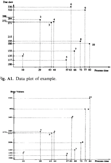
Fig. Al. Data plot of example.
Appendix
The example below illustrates the steps of the algorithm BETA.
Suppose we have 10 jobs to schedule corresponding to the data plotted in Fig, A I. According to the steps of the algorithm, we first apply LEFT to obtain the /i-sequence (5, 1,7,8,3,4,2,6,9,10) shown in Fig. A2,
Jobs 5, 1,7,8,3,4 pass the fJ-test, but job 2 fails. Since we find at least one job failing, we cannot conclude that the /i-sequence is optimum, Then we look at the exact decomposition and try to decompose if possible. From Fig, Al we see that RD7
=
0. This means that the first condition of the exact decomposition theorem is satisfied. Since LU7=
{2, 3,4, 6} the second condition to check is ifPi
+
/ii2:
L7 ViE LU7 and we find that the inequality is valid for all the jobs in LU7. Thus the problemdecom-poses with job 7 at position 3 forming two subproblems. One problem has only two jobs {I, 5} and the other problem has 7 jobs {2, 3, 4, 6, 8, 9, 1O}.
For the two job case we can easily find the optimum sequence. Ithappens to be (5, I). For the second problem we apply the algorithm once more. The /i-sequence con-structed for this subproblem is (8, 3,4,2,6,9, 10), We try the /i-test first. The test fails so we try exact decomposi-tion. Note that the right-down and left-up sets of job 9 are empty. Hence, the problem decomposes with job 9 at position 6, with job lOin the up-set and the others in the set. After the decomposition with job 9, the down-set {2, 3,4,6, 8} will be solved. Itdecomposes with job 6 in the last position, At this stage, jobs 7,9,6 are already in fixed positions (these are the jobs that qualified for exact
Rinnooy Kan, A.H.G., Lageweg, B.J. and Lenstra, J.K. (1975) Mini-mizing total costs in one machine scheduling. Operations Re-search, 23, 908-927.
Schrage,L.and Baker, K.R. (1978) Dynamic programming solution of sequencing problems with precedence constraints. Operations
Research, 26,444-449.
Schwimer, J. (1972) On the 11job one machine sequence independent scheduling with tardiness penalties: a branch and bound solution.
Management Science, 18,301-313.
Sen, T.T., Austin, L.M. and Ghandforoush, P. (1983) An algorithm for the single machine sequencing problem to minimize total tardi-ness. IfE Transactions, 15, 363-366.
Sen, T,T. and Borah, B.N. (1991) On the single machine scheduling problem with tardiness penalties. Journal of the Operational
Re-search Society,42, 695-702.
Srinivasan. V. (1971) A hybrid algorithm for the one machine se-quencing problem to minimize total tardiness. Naval Research Logistics Quarter!", 18, 317-327.
Szwarc, W. and Mukhopadhyay, S.K. (1996) Decomposition of the single machine total tardiness problem. Operations Research
Letters, 19, 243-250.
Tansel, B.C. and Sabuncuoglu, I. (1997) New insights on the single machine total tardiness problem. Journal of the Operational
Research Society, 48, 82-89.
Wilkerson, J.1. and Irwin, J.D. (1971) An improved method for scheduling independent tasks. A If E Transactions, 3, 239-245.
jobs 2,3,4 are to be scheduled before it. The second branch yields an optimum for its subproblem which is no better than the first branch. Hence, the final optimum sequence is (5, 1,7,8,3,2,4,6,9,10).
Biographies
Barburos C. Tansel is the Chairman of the Department of Industrial Engineering at Bilkent University. Ankara. Turkey. Dr. Tansel earned his Ph.D. degree in 1979 from the University of Florida. Department of
Industrial andSystems Engineering. Prior to his appointment at Bil-kent University in 1991. he was a visiting faeuity member at the Georgia Institute of Technology and a faculty member at the Uni-versity of Southern California. Dr. Tanscl's primary research interests
arc in location theory, combinatorial optimization, and optimization
with imprecise data. He has published in various journals including
Operations Research, Management Science, Transportation Science,
European Journal of OperationalResearch, Journal of the Operotional
Research Society. international Journal ()fProduction Research, and
JournalofManufacturing Systems.
Bahar Y. Kant received her Ph.D. degree in 1999 from Bilkent Uni-vcrsity, Department of Industrial Engineering. Since then. Dr. Kara has worked as a Post-Doctoral Research Fellow at McGill University,
Faculty of Management. Her primary research interests are in hub location, hazardous materials transportation. discrete optimization. and bilevel programming.
Ihsan Sabuneuoglu is an Associate Professor of Industrial Engineering at Bilkcnt University. He received B.S. and M.S. degrees in Industrial Engineering from the Middle East Technical University and a Ph.D. degree in Industrial Engineering from Wichita State University. Dr. Sabuneuoglu teaches and conducts research in the areas of scheduling,
production management, simulation, and manufacturing systems. He has published papers in 11E Transactions, Decision Sciences,
Simula-tion, International Journal of Production Research,InternationalJournal
of Flexible Manufacturing Systems, International Journal of Computer
IntegratedManufacturing, European Journal of Operational Research,
Production Planning and Control, Journal of the Operational Research Society, Computers and Operations Research. Computers and Industrial
Engineering. OMEGA, Journal of Intelligent Manufacturingand Inter-national Journal of Production Economics. He is on the Editorial board
of International Journal of Operations and Quantitative Management
and also the Journal of Operations Management. He is an associate member of Institute of Industrial Engineering. Institute of Simulation. and Institute of Operations Research and Management Science.