PDF NOVEL SWARM INTELLIGENCE ALGORITHMS FOR STRUCTURE LEARNING OF ... - Yasar

YAŞAR UNIVERSITY

GRADUATE SCHOOL OF NATURAL AND APPLIED SCIENCES

PHD THESIS

NOVEL SWARM INTELLIGENCE ALGORITHMS FOR STRUCTURE LEARNING OF BAYESIAN NETWORKS

AND A COMPARATIVE EVALUATION

SHAHAB WAHHAB KAREEM

THESIS ADVISOR: PROF. DR. MEHMET CUDI OKUR

PHD WITH THESIS IN ENGLISH

PRESENTATION DATE: 07.01.2020

ABSTRACT

NOVEL SWARM INTELLIGENCE ALGORITHMS FOR STRUCTURE LEARNING OF BAYESIAN NETWORKS AND A COMPARATIVE

EVALUATION

Kareem, Shahab Wahhab Ph.D, Computer Engineering Advisor: Prof.Dr.Mehmet Cudi Okur

January 2020

Bayesian networks are useful analytical models for designing the structure of knowledge in machine learning which can represent probabilistic dependency relationships among the variables. A Bayesian network depends on; 1.the parameters of the network and 2.the structure. Parameters represent conditional probabilities while the structure represents dependencies between the random variables. The structure of a Bayesian network is a directed acyclic graph (DAG). Learning the structure of a Bayesian network is NP-hard but still extensive work have been done to optimize approximate solutions. In this thesis, we have conducted research for structure learning to develop algorithms to find a solution to the problem. There are two approaches for learning the structure of Bayesian networks. The first is a constraint-based approach, and the second is a score and a search approach. One common type of method for Bayesian network structure learning is the score-based search. Score-based methods rely on a function to test how well the network model matches the data, and they search for a structure that produces high scores on this function. There are two types of scoring functions: Bayesian score and information-theoretic score. The Bayesian and information-theoretic scores have been implemented in several structure learning methods. In this thesis, we focused on the score based search for testing the structure learning of Bayesian network using heuristic methods for searching and BDeu as a score function. In this thesis we proposed five algorithms for the search part and used BDeu as a score function. We also proposed a sixth method which is also a nature inspired one. The first proposed algorithm used Pigeon Inspired Optimization as a search method and the above mentioned score function. The proposed method has shown a good result when compared with default methods like Simulated Annealing

and greedy search. This algorithm is a novel approach applied for structure learning of Bayesian network. The second proposed algorithm used Bee optimization and Simulated Annealing as a hybrid algorithm, which used Bee optimization as a local search and Simulated Annealing as a global search. The third proposed algorithm also used bee optimization and Simulated Annealing as a hybrid but used Bee optimization as a global search and Simulated Annealing as a local search. The fourth proposed algorithm used Bee optimization and Greedy search as a hybrid algorithm. It used Bee optimization as local search and Greedy as global search. The fifth algorithms also used bee optimization and Greedy as a hybrid algorithm, but it used Bee optimization as a global search and Greedy as a local search Our last proposed algorithm used Elephant Swarm Water Search Algorithm (ESWSA). The thesis presents the results of extensive evaluations of these algorithms based on common benchmark data sets.

Applications of ESWSA in Structure learning of Bayesian Network and comparisons with the Simulated Annealing and Greedy Search, show that this proposed method is better than the default Simulated Annealing and Greedy search methods.

Keywords: Bayesian network, structure learning, Pigeon Inspired Optimization, Bee Optimization, greedy, Simulated Annealing, elephant swarm search, water search, global search, local search, search and score.

ÖZ

BAYES AĞ YAPILARININ ÖĞRENİLMESİ İÇİN YENİ SÜRÜ ZEKASI ALGORİTMALARI VE KARŞILAŞTIRMALI BİR DEĞERLENDİRME

KAREEM, SHAHAB WAHHAB Doktora Tezi, Bilgisayar Mühendisliği Danışman: Prof.Dr.Mehmet Cudi Okur

Ocak 2020

Bayes ağları, makina öğrenmesinde değişkenler arasındaki rassal ilişkileri temsil eden bilgi yapısının tasarımında kullanılan yararlı analitik modellerdir. Genel olarak Bayes ağı Ağın Parametreleri ve Ağın yapısına bağlıdır.Parametreler şartlı olasılıkları,yapı ise şans değişkenleri arasındaki bağımlılıkları temsil eder. Bir Bayes ağının yapısı yönlü çevrimsel olmayan bir çizgedir.Bayes ağının yapısını öğrenmek bir NP-zor problem olmasına ragmen,yaklaşık çözümlerin eniyilenmesi için çok sayıda geniş kapsamlı çalışmalar yapılmıştır.Bu tezde yapı öğrenme problemine çözüm bulmayı amaçlayan algoritmalar geliştirmek için araştırmalar yürütülmüştür.Bayes ağların yapısın öğrenmek için iki yaklaşım vardır.Birinci yaklaşım kısıtlamalı diğeri ise skor ve arama temellidir.Skor temelli yaklaşımlar genel yaklaşımlardır.Bu yaklaşımlar ağ modelinin verilere nasıl uyum gösterdiğni ölçen bir fonksiyonu esas alırlar ve bu fonıksiyonun değerini daha iyileştirecek yapıyı üretmeye çalışırlar.İki tür skor fonksiyonu vardır :Bayesçi skor ve bilgi teorisi skoru. Her iki skor da yapı öğrenme yöntemlerinde uygulanmıştır.Bu tezde Bayes ağın yapısını öğrenmede skor temelli arama için sezgisel yötemler kullanılmış ve skor fonksiyonu olarak BDeu metriği kullanılmıştır.Bu amaçla,BDeu yu kullanan altı algoritma önerimiştir.Önerilen ilk algoritma güvercinlerin yön bulmasından esinlenen eniyileme algoritmasıdır ve BDeu skorunu kullanmaktadır.Önerilen yöntemin yaygın kullanılan yöntemlerden daha iyi sonuçlar verdiği görülmüştür.Bu algoritma bu alanda ilk defa kullanılmaktadır.İkinci önerilen algoritma arı eniyilemesi algoritmasına ve benzetilmiş tavlama algoritmasına dayanmakta ve ilkini global ikincisini de yerel arama için kullanmaktadır.Üçüncü önerilen yöntem gene önceki ikisini esas almakta fakat bu defa arı eniyilemesi global,

benzetilmiş tavlama algoritması yerel arama için kullanılmıştır. Dördüncü önerilen yöntemde melez bir yöntem olup arı eniyilemesi ve açgözlü amayı esas almakta ve arı eniyilemesini yerel ve açgözlüyü de global arama için kullnmaktadır.Beşinci yöntem de melezdir ve arı eniyilemesini global,açgözlü yöntemi yerel arama için kullanmaktadır.Son önerimiz Fil sürülerinin su kaynağı arama algoritmasına dayanmaktadır.Tezde genel kıyaslama veri setleri kullanılarak BDeu metriği ve karışıklık matrislerine dayanan değerlendirmeler tartışılmış, sonuçta güvercin yön bulma ve fil sürüleri su arama yöntemlerine dayanan algoritmaların diğerlerindan daha başarılı olduğu gösterimiştir.

Anahtar sözcükler: Bayes ağı,yapı öğrenme,Güvercinden Esinlenen Algoritma,Arı Eniyilemesi,açgözlü,Benzetilmiş Tavlama,,Fil sürü araması,su araması,global arama,yerel arama, arama ve skor.

ACKNOWLEDGEMENTS

First of all, I would like to thank my supervisor PROF. DR. MEHMET CUDİ OKUR for his guidance and patience during this study.

I would like to express my enduring love to my Wife, Childs, Parents, Sisters and brother who are always supportive, loving and caring to me in every possible way in my life.

Shahab Wahhab Kareem İzmir, 2020

TEXT OF OATH

I declare and honestly confirm that my study, titled “Novel Swarm Intelligence Algorithms for Structure Learning of Bayesian Networks and a Comparative Evaluation” and presented as a PhD Thesis, has been written without applying to any assistance inconsistent with scientific ethics and traditions. I declare, to the best of my knowledge and belief, that all content and ideas drawn directly or indirectly from external sources are indicated in the text and listed in the list of references.

Shahab Wahhab Kareem Signature

………..

January 9, 202020

TABLE OF CONTENTS

ABSTRACT ... i

ÖZ ... iii

ACKNOWLEDGEMENTS ... vi

TEXT OF OATH ... vii

TABLE OF CONTENTS ... ix

LIST OF FIGURES ... xii

LIST OF TABLES ... xiv

ABBREVIATIONS ... xvii

CHAPTER 1 INTRODUCTION ... 1

1.1. MOTIVATION...1

1.2. THESIS GOALS AND OVERVIEW...3

1.3. THESIS ORGANIZATION...4

CHAPTER 2 BAYESIAN NETWORK...5

2.1 STATISTICAL MODELLING...5

2.1.1 PROBABILITY ...6

2.1.2 CONDITIONAL PROBABILITY ... 6

2.1.3 BAYES RULE ... 7

2.1.4 INDEPENDENCE ... 7

2.2 GRAPH THEORY AND BAYESIAN NETWORKS... 8

2.2.1 GRAPHS, NODES, AND ARCS... ...8

2.2.2 THE STRUCTURE OF A GRAPH...9

2.3 PROBABILISTIC GRAPHICAL MODELS...10

2.3.1 MARKOV NETWORKS...12

2.3.2 BAYESIAN NETWORKS...12

2.3.3 SOME PRINCIPLES OF BAYESIAN NETWORK ...13

2.3.3.1 D-SEPARATION ...13

2.3.3.2 MARKOV EQUIVALENT CLASS ...14

2.3.4 QUERYING A DISTRIBUTION...15

2.3.4.1 EXACT INFERENCE...16

2.3.4.2 APPROXIMATE INFERENCE...16

2.4 BAYESIAN NETWORK LEARNING...17

2.4.1 LEARNING THE STRUCTURE OF BAYESIAN NETWORKS ...20

2.4.1.1 THE SCHEMA FOR LEARNING STRUCTURE...22

2.4.1.2 PROCEDURE FOR LEARNING STRUCTURE...23

2.4.1.3 THE COMPLEXITY OF STRUCTURE LEARNING...25

2.4.1.4 CONSTRAINT BASED METHODS...25

2.4.1.5 SCORE-AND-SEARCH BASED METHODS...28

2.4.1.6 HYBRID METHOD ...36

2.5. EVALUATING STRUCTURAL ACCURACY...38

2.5.1 EVALUATION METRICS...38

2.5.2 CONFUSION MATRIX...39

2.5.2.1 ACCURACY ANT ERROR RATE...40

2.5.2.2 SENSITIVITY AND SPECIFICITY...40

2.5.2.3 PRECISION, RECALL AND F-SCORE...42

CHAPTER 3 PROPOSED ALGORITHMS ...44

3.1. PIGEON INSPIRED OPTIMIZATION ...44

3.1.1 OVERVIEW OF PIGEON INSPIRED OPTIMIZATION...45

3.1.2 MATHEMATICAL MODEL OF PIO...46

3.2. SIMULATED ANNEALING... 49

3.2.1 INTRODUCTION OF SIMULATED ANNEALING...49

3.2.2 SIMULATED ANNEALING ALGORITHM...50

3.2.3 IMPLEMENTATION OF THE S.A. ALGORITHM...52

3.3. GREEDY ALGORITHMS ...53

3.3.1 ELEMENTS OF THE GREEDY STRATEGY...54

3.3.2 OPTIMAL SUBSTRUCTURE. ... ...56

3.4. BEE ALGORITHMS ...56

3.4.1 BEES IN NATURE... ... ...57

3.4.2 ARTIFICIAL BEES...58

3.4.3. BEE ALGORITHM...59

3.5. NATURE INSPIRED ELEPHANT SWARM WATER SEARCH ALGORITHM...61

3.5.1 ELEPLANT IN NATURE...61

3.5.2 SOCIAL BEHAVIOR AND INTERACTION IN ELEPHANTS...63

3.5.3.ELEPHANT SWARM WATER SEARCH ALGORITHM ...64

3.6. METHODOLOGY...67

3.6.1. FIRST PROPOSED METHOD...67

3.6.2. SECOND PROPOSED METHOD...71

3.6.3. THIRD PROPOSED METHOD...75

3.6.4. FOURTH PROPOSED METHOD...78

3.6.5. FIFTH PROPOSED METHOD...80

3.6.6. SIXTH PROPOSED METHOD...83

CHAPTER 4 DATASETS AND EXPERIMENTS ...87

4.1. DATASETS ...87

4.2. EXPERIMENTAL RESULT OF SCORE FUNCTION ...89

4.3. EXPERIMENTAL RESULT OF CONFUSION MATRIX...98

CHAPTER 5 CONCLUSIONS AND FUTURE RESEARCH ... 116

REFERENCES ... 122

LIST OF FIGURES

Figure 2.1. Directed, undirected, and partially directed ... 8

Figure 2.2. Parents, neighbors, ancestors, children, and descendants, of a node within a directed graph ... 10

Figure 2.3. Conditional independence: (a) DAG as an example. (b) Markov random field (MRF) as an example. ... 11

Figure 2.4. The Model of Bayesian network; A DAG among parameters and nodes describing the probability distribution. ... 13

Figure 2.5. Head-to-tail or Serial relation ... 13

Figure 2.6. Head-to-head or Converging relation ... 14

Figure 2.7. Tail-to-tail or Diverging connection ... 14

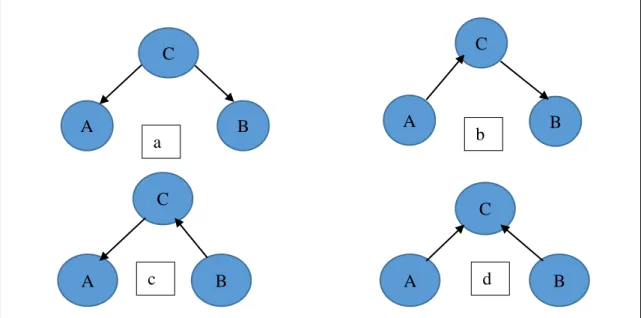
Figure 2.8. An example of Markov equivalent class for three variables, , A, B, C, and four DAGs. The (a), (b) and (c) DAGs have a similar independence structure while (d) compares to a different set of independencies………..15

Figure 3.1 Map and compass operator model of PIO ... 47

Figure 3.2 Landmark operator model ... 47

Figure 3.3 Flowchart of the Simulated Annealing algorithm ... 49

Figure 3. 4Pseudo-code of a greedy algorithm for a minimization problem ... 54

Figure 3. 5 Pseudo code of the basic bees algorithm ... 59

Figure 3. 6 The Bees Algorithm Flowchart ... 60

Figure 3. 7 Group exhibitions in Elephants clan ... 62

Figure 3. 8 Pseudo Code of The PIO for Structure Learning Bayesian Network ... 69

Figure 3. 9 Map and compass steps for one Pigeon ... 70

Figure 3. 10 Pseudo code of BSA hybrid bee local and SA is global search ... 74

Figure 3. 11 Pseudo code SAB (Bee global search and SA is local search) ... 76

Figure 3. 12 Pseudo code BLGG (Bee local search and Greedy is global search). ... 79

Figure 3. 13 The construction process of a Bayesian Network ... 80

Figure 3. 14 Pseudo code BGGL (Bee global search and Greedy is local search) ... 82

Figure 3. 15 The construction process of a BN. ... .83

Figure 3. 16 ESWSA Algorithm for Structure learning Bayesian Network. ... .85

Figure 3. 17 Water searching steps for one Elephant ... 86

Figure 4.1 Sensitivity of PIO and Simulated Annealing and Greedy ... 99

Figure 4.2 Accuracy of PIO and Simulated Annealing and Greedy ... 100

Figure 4.3 F1_Score of PIO and Simulated Annealing and Greedy ... 100

Figure 4.4 AHD of PIO and Simulated Annealing and Greedy ... 101

Figure 4.5 PPV for BSA, SAB, and Simulated Annealing ... 102

Figure 4.6 Sensitivity for BSA, SAB, and Simulated Annealing ... 103

Figure 4.7 Accuracy for BSA, SAB, and Simulated Annealing ... 103

Figure 4.8 F1_Score for BSA, SAB, and Simulated Annealing ... 104

Figure 4.9 AHD for BSA, SAB, and Simulated Annealing ... 104

Figure 4.10 PPV for BLGG, BGGL and Greedy ... 106

Figure 4.11 Sensitivity for BLGG, BGGL and Greedy ... 106

Figure 4.12 Accuracy for BLGG, BGGL and Greedy ... 107

Figure 4.13 F1_Score for BLGG, BGGL and Greedy ... 107

Figure 4.14 AHD for BLGG, BGGL and Greedy ... 108

Figure 4.15 Sensitivity for ESWSA, Simulated Annealing, and Greedy ... 110

Figure 4.16 Accuracy for ESWSA, Simulated Annealing, and Greedy ... 110

Figure 4.17 F1 Score for ESWSA, Simulated Annealing, and Greedy ... 111

Figure 4.18 AHD for ESWSA, Simulated Annealing, and Greedy ... 112

Figure 4.19 Sensitivity for Proposed Methods ... 114

Figure 4.20 Accuracy for proposed Methods ... 114

Figure 4.21 F1 Score for proposed Methods ... 115

Figure 4.22 AHD for Proposed Methods ... 115

LIST OF TABLES

Table 2.1. The table presents the amount of various DAGs that can produce several nodes.

For example, there are 1.4*10⁴¹ different DAGs with 14 nodes ... 21

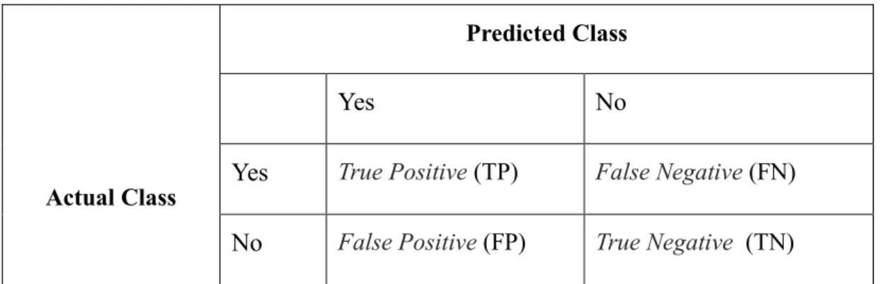
Table 2.2. Confusion Matrix . ... 39

Table 2.3. Test result in Confusion matrix . ... 41

Table 2.4. Sensitivity and Specificity in Confusion matrix ... 42

Table 3.1. Designing the S.A. Algorithm . ... 52

Table 4.1. Calculation results of the best of BDeu Score function for PIO with Simulated Annealing and Greedy in 2 minutes Execution time . ... 90

Table 4.2. Calculation results of the best of BDeu Score function for PIO with Simulate Annealing and Greedy in 5 minutes Execution time . ... 90

Table 4.3. Calculation results of the best of BDeu Score function for PIO with Simulate Annealing and Greedy in 60 minutes Execution time . ... 90

Table 4.4. Calculation results of the best of BDeu Score function for BSA and SAB with Simulate Annealing in 2 minutes Execution time . ... 91

Table 4.5. Calculation results of the best of BDeu Score function for BSA and SAB with Simulate Annealing in 5 minutes Execution time . ... 91

Table 4.6. Calculation results of the best of BDeu Score function for BSA and SAB with Simulate Annealing in 60 minutes Execution time . ... 92

Table 4.7. Calculation results of the best of BDeu Score function for BLGG and BLGG with defualt Greedy in 2 minutes Execution time . ... 92

Table 4.8. Calculation results of the best of BDeu Score function for BLGG and BLGG with defualt Greedy in 5 minutes Execution time . ... 93

Table 4.9. Calculation results of the best of BDeu Score function for BLGG and BLGG with defualt Greedy in 60 minutes Execution time . ... 93

Table 4.10. Calculation results of the best of BDeu Score function for ESWSA, Simulated Annealing, and Greedy in 2 minutes Execution time. ... 94

Table 4.11. Calculation results of the best of BDeu Score function for ESWSA, Simulated

Annealing, and Greedy in 5 minutes Execution time ... 95

Table 4.12. Calculation results of the best of BDeu Score function for ESWSA, Simulated Annealing, and Greedy in 60 minutes Execution time. ... 95

Table 4.13. Calculation results of the best of BDeu Score function for all proposed methos when time is 2M. ... 96

Table 4.14. Calculation results of the best of BDeu Score function for all proposed methos when time is 5M ... 97

Table 4.15. Calculation results of the best of BDeu Score function for all proposed methos when time is 60 M. ... 97

Table 4.16. Confusion matrix of PIO, Simulated Annealing and Greedy ... 99

Table 4.17. Confusion matrix of BSA, SAB, and Simulated Annealing. ... 102

Table 4.18. Confusion matrix of BLGG, BGGL, and Greedy. ... 105

Table 4.19. Confusion matrix of ESWSA, Simulated Annealing, and Greedy... 109

Table 4.20. Confusion matrix of All proposed methods. ... 113

ABBREVIATIONS

ABC Artificial Bee Colony Optimization ACO Ant Colony Optimization

AIC Akaike information criterion BA Bee Algorithm

BD Bayesian Dirichlet

BDe Bayesian Dirichlet (“e” for likelihood-equivalence)

BDeu Bayesian Dirichlet equivalent uniform (“u” for uniform joint distribution) BFO Bacterial Foraging Optimization

BGeu Bayesian Gaussian equivalent uniform

BGGL Greedy as local search and Bee as global search BIC Bayesian Information Criterion

BLGG Bees as local search and Greedy as global search BN Bayesian Network

BP Backpropagation

BSA Bees as local search and Simulated Annealing as global search CF Cell Formation

CM Cellular manufacturing CPT Conditional Probability Table DAG Directed Acyclic Graph.

EF Employed forager ER Recruit unconvertable

ESWSA Elephant Swarm Water Search Algorithm ES Scout begins for the exploration

FN False Negative FP False Positive GS Greedy Search

IAMB Incremental Association Markov blanket algorithm IC Inductive Causation

KDD Knowledge from Data Discovery

LL Log-likelihood

MAP Maximum a Posteriori

MAP Maximum a Posteriori Probability MB Markov Blanket

MDL Minimum Description Length MIT Mutual Information Tests MLP Multi-layered Perceptron

MMHC Original Max-Min Hill-Climbing algorithm MMPC Max-Min Parent Children

MRF Markov Random Fields

NML Normalized Minimum Likelihood P Precision

P(V) Probability Distribution PC Parent-Children

PCB Printed Circuit Board

PDF Probability Density Function PGM Probabilistic graphical models PIO Pigeon Inspired Optimization PMF Probability Mass Function PSO Particle Swarm Optimization

R Recall

R Recruit

RCE Randomized Control Experiment RF Reactivated forager

S Scout

SA Simulated Annealing

SAB Simulated Annealing as local search and Bee as global search SC Sparse Candidate

SVM Support Vector Machine TN True Negative

TP True Positive

TP True Positive

P(x) The probability of event X X∩Y The crossing between X and Y

P(X|Y) The probability of the event X, given that Y has happened u→ v Directed of u to v

θ The probability distributions of any random variable

ΠXi Parent of xi

Γ Gamma Function

CHAPTER 1 INTRODUCTION 1.1. Motivation

Machine Learning involves techniques for computers programming to learn. Machines used to achieve a universal variety concerning responsibilities, including the development of needed software for most computational tasks. Machine learning approaches deal with several of the related study topics such as the domains of data mining, artificial intelligence and statistics. Data mining explores models within some data which is recognizable by people. Statistics concentrates on explaining the events that are present in experimental or observational data sets [1] [2]. Majority of the researches use data mining methods to train observed data and to extract intelligence rules. With specific rules, it obtains a probabilistic graphics model, statistical models, Bayesian statistics, and machine learning. Graphics models combine probability and graph theory. It’s present a simplistic mechanism as dealing including difficulties that arise while coupling engineering and mathematics to reduce ambiguity and complexity.

As such, they play a significant role in machine learning algorithms during steps design and analysis. The theory of probability presents methods to analyze how the components joined, guaranteeing that the system remains consistent. The combined results expected to be compatible and present new techniques to propose new interface models for observed data. Some graph-theoretic view of graphical models presents an attractive interface jointly for users that ability to create reactive collections about variables and a data structure that can be used in powerful public-objective algorithms[2]. One of the most important types for probabilistic graphical models is the Bayesian Network [3, 4]. They commonly used in the field of Knowledge from Data Discovery (KDD). A Bayesian network is a directed acyclic graph whose nodes (vertices) describe links and variables (or controlled arcs) show the statistical relationship among variables and a probability distribution defined across those variables. An essential difficulty of the modern study is Bayesian network learning from observed data. The development of principles can be performed both by utilising observed data or expertise. Several kinds of research have been conducted on this subject, deriving on various approaches: Techniques to the development regarding independence structure within data to rebuild for optimizing an actual function of the

graph, namely a score. Optimization techniques aim to the development of a representation of the local structure based on a destination variable to rebuild the network of the global structure. Most researches have restricted their work to static cases for learning the structure of Bayesian networks. The majority of these algorithms use a traditional approach which depended on scores.

In the rest of this thesis, we consider the combination of strategies, namely, global optimization and local search relating the static case. We remarked that the structure learning Bayesian network is a well-researched field. To our knowledge, the researcher about BN structure learning applies the benchmarks to evaluate the procedures. The difficulty in the Bayesian network structure learning instance is the search for discovering the excellent structure. But, this depends on the score and search method, which is computationally NP-hard. Furthermore, causal models can offer enough extra benefits for researchers. It can assist us in experiencing our situation and identifying “laws” of the environment in the Sciences: Chemistry, Biology, Physics, even Genetics. Growing developments under a related thread now can and make for example, scientists to limit the options of the analysis for infections. In that space, the building of patterns automatic or the semi-automatic can be valuable. In the dissertation, we preferred to concentrate on covering structure learning of Bayesian network depending on the score and search method. Different models can describe possible domains—as an example, artificial neural networks, decision trees, Markov networks, blend of essential roles, etc. The researcher in Bayesian Network describes and learn directed causal connections, which is also our final purpose. We attempt to explain the combinatorial difficulty of getting the most significant scoring from data in the Bayesian network structure. This can be view as the challenge of structured learning which is as an inference difficulty. The major combinatorial problem drives from the global constraint that the structure of the graph has to be acyclic. The problem of the structure learning may be called as a linear program covering the polytope described by logical acyclic structures. To decrease the mentioned difficulties through applying a restricted external approach to the polytope which stretch it through exploring the validity constraints. In Case of finding the full solution, it has proven to be the optimal solution of the Bayesian network. Alternative approaches are; Pigeon Inspired Optimization, simulated annealing, the greedy method and Elephant Swarm Water Search algorithms.

1.2. THESIS GOALS AND OVERVIEW

A Bayesian network (BN) involves common useful theoretical principles to describe the possibility of learning from data in artificial intelligence. A graphical model used by Bayesian Network for representing the conditional dependency connections between arbitrary variables and those variables governed by the joint probability distribution [3]. Assume a Bayesian Network and observations for many variables are given, a probabilistic inference can then determine the fitness of the other unobserved variables. Systems accept this standard to design solutions to practical difficulties within various domains, such as biology, medical diagnosis, natural language processing, control, and forecasting [4].

Learning the structure automatically from the data, attracted researchers and several learning algorithms have become available [5, 6, 7, 8, 9, 10, 11, 12, 13, 14]. [15, 16, 17, 18, 19, 20, 21, 22, 23, 24] [25, 26, 27, 28]. Those algorithms choose the score and search, or the dependency analysis approaches. Dependency analysis applies a statistical method for finding dependency and independence connections between variables and whereby constructs a Bayesian Network [10]. Applying a search technique in the score and search approaches to investigate Bayesian Network structures aims to find the highest score value achieved [18]. Both methods have severe disadvantages. Dependency analysis requires dealing with a massive number of cases that are difficult also unpredictable; moreover, it is challenging to guarantee the quality properties of learning. In contrast, Bayesian Network structure learning through the score and search is an NP-hard problem because of the number of variable increments [29]. Once the location of applicant networks grows high, exact search results may be unsuitable for structural learning in Bayesian Network. While some heuristic algorithms, like hill-climbing algorithms [30, 31], K2 [32], repeated local search [33, 34], can mark the difficulty of significant search areas, they grow confined within local optima.

To explore those difficulties, many stochastic algorithms have proposed for the Bayesian Network structure learning during the last years. [35]. We Can classify those algorithms within two classes [33]:

1. Swarm intelligence algorithms, which are nature-inspired optimization procedures that include bacterial foraging optimization (BFO) [5], artificial

Bee colony optimization (ABC) [7], ant colony optimization (ACO) [15, 36], particle swarm optimization (PSO) [16], artificial fish swarm algorithm [37].

They utilize a meta-heuristic search technique in search space of the Bayesian Network and use a scoring function for determining the best of the applied networks.

2. The evolutionary algorithms which represent an inspiration of evolution including common genetics and also genetic programming, genetic algorithm, which involve evolutionary programming, and evolution strategy. Genetic algorithm [38] and evolutionary programming [31] are standard techniques which are useful approaches for Bayesian Network structure learning from data.

1.3. THESIS ORGANIZATION

This study concentrates on the structure learning of Bayesian network. First chapter includes a literature review of structure learning of Bayesian networks based on score and the search approach. The basic principles of Bayesian networks and structure learning of Bayesian networks explained in Chapter 2. The Pigeon Inspired optimization, Elephant Swarm Water Search Algorithm, Bees algorithm, Simulated Annealing, Greedy Search and proposed algorithms for structure learning of Bayesian networks explained in Chapter 3. Chapter 4 concentrates on the results obtained from the implementations of various algorithms that we proposed. Conclusions and recommendations for future studies presented in Chapter 5.

CHAPTER 2

BAYESIAN NETWORK

Knowledge description and thinking of these descriptions have caused the development of several models. Bayesian networks, and Probabilistic graphical models, have been established to be valuable instruments as a description of ambiguous knowledge. Then, many researchers such as [39, 40, 41, 42] proposed a Bayesian probabilistic reasoning formalism for knowledge extraction from incomplete information.

Learning a Bayesian network is composed of two states: parameter learning and structure learning. In this thesis, our focus is on structure learning of Bayesian networks. There are three kinds of techniques in structure learning: techniques depending on a description of conditional independence, techniques depending on optimization like score also hybrid approaches.

To illustrate the advantages of structure learning algorithms, these learning algorithms should tested using the achieved properties of the corresponding Bayesian networks.

Some algorithms use several evaluation metrics in search and identify the network through an application of the score-based methods. Some others concentrate on the application of a source form. In our thesis, we concentrated on specific evaluation procedures utilising a score-based method.

This chapter reviews fundamental descriptions and representations of traditional Bayesian networks, probability and conditional independence.

2.1 STATISTICAL MODELLING

Usually, statistical modelling strategies utilised within several systems to describe complicated multi-parametric structures. The probabilistic form shows an ontological framework; also, it represents the relationships with the model’s fundamental entities.

Unlike deterministic models, where the links are explained by mathematical equations (either science-based or derived), in statistical models the connections among variables are probabilistic. In the subsequent sections, we present the principle of probability, conditional and marginal probability distributions and their use in the graphical models that underpin the Bayesian structure learning methods.

2.1.1 PROBABILITY

A traditional frequency-based explanation of probability is the following: Probability of a disjoint event is the occurrence frequency of this event compared to the cumulative amount of times the events can happen. Suppose, for instance, the analysis conducted several times, and each time a result is one of three events A, B or C. If the number of their occurrences are 𝑛_𝐴 , 𝑛_𝐵 , 𝑛_𝐶 the probability of event A is then presented by the following Equation [43].

𝑃(X) = _{(𝑛𝐴 +𝑛}^𝑛_𝐵^𝐴 _{+ 𝑛𝐶)} Equation 2-1

Bayesian or most frequent likelihood test based on the three necessary assumptions of probability analysis [44]. First, a probability cannot be larger than one and smaller than zero (Equation 2-2). If that is one, the event will occur; zero means the event will never happen.

0 ≤ 𝑃(X) ≤ 1 Equation 2-2

In a unit space S, comprising a measurable number of fundamental events there is a total likelihood that one of the fundamental events will happen

𝑃(𝑆) = 1 Equation 2-3

Wherever events are disjoint, the cumulative probability of one or another of the events happening can be obtained by the sum of their specific probabilities

𝑃 (X ∪ Y) = 𝑃(X) + 𝑃(Y) Equation 2-4

If the events can both happen, the probability of both events happening can be obtained by the Equation:

𝑃 (X ∪ Y) = 𝑃(X) + 𝑃(Y) − 𝑃 (X ∩ Y) Equation 2-5

Where X∩Y denotes the intersection between X and Y, which is the event that both X and Y happen [43].

2.1.2 CONDITIONAL PROBABILITY

Conditional probability interprets the occurrence probability of an event, given some other event has already occurred. The probability of the event X, given that Y has happened shown as 𝑃(X|Y) and described by:

𝑃(X|Y) = 𝑃 (X ∩ Y) / 𝑃(Y) Equation 2-6

This is known as the primary rule of conditional probability. Equation 2-6 can express as

𝑃 (X ∩ Y) = 𝑃(Y).𝑃(X|Y) Equation 2-7 The conditional probability definition can extend to cover more joint events as in Equation 2-8.

𝑃(X ∩ Y ∩ Z) = 𝑃(X|(Y ∩ Z) ⋅ 𝑃(Y ∩ Z) Equation 2-8 = 𝑃(X|(Y∩ Z) ⋅ 𝑃(Y|Z) ∙ P(Z)

The Equation 2-8 is the chain rule and expressed for n joint events in Equation 2-9.

This rule is essential for factorizations in probability analysis of Bayesian Networks.

𝑃(∩_𝑖=1^𝑛 𝑋_𝑖) = ∏^𝑛_𝑖=1P(𝑋_𝑖| ∩_𝑖=1^𝑛 𝑋_𝑖) Equation 2-9 Bayesian probability declares that every probability is conditional upon specific situations under which determinations performed or operations executed [45].

2.1.3 BAYES RULE

Considering, from the assumptions of probability 𝐴∩𝐵≡𝐵∩𝐴, also from the primary rule, the connection between conditional probabilities can express as in Equation 2-10.

𝑃(X|Y) = 𝑃(𝑌|𝑋) ⋅ 𝑃(𝑋)

P(Y) Equation 2-10 The formula, identified as Bayes rule, defined posthumously in a historical form in 1763. It provides a posterior probability, P(X|Y), given any extra information, Y, which is identified as the prior probability, 𝑃(X).

2.1.4 INDEPENDENCE

Independence of two events implies that the occurrence of one event is not influenced by the occurrence of another event. Thus the independence of the events X and Y are expressed by Equation 2-11.

𝑃(X|Y) = 𝑃(X) Equation 2-11

Using the fundamental conditional probability rule, Equation 2-12 follows.

𝑃(X ∩ Y) = 𝑃(X) ⋅ 𝑃(Y) Equation 2-12 2.2 GRAPH THEORY AND BAYESIAN NETWORKS

2.2.1. GRAPHS, NODES, AND ARCS

A graph G = (V, A) composed from a non-empty collection V of vertices or nodes also a limited (however probably empty) collection A of edges, or links. Each edge X = (u, v) describes essentially a couple of neighboring nodes. The nodes are joined by an arc which represents a weight value. If in (u, v), order is important, they represent a directed arc or edge. The arc is assumed to direct the link of u to v also generally described by an arrowhead as (u→ v). It is an additional assumption that the arc moves or are outgoing from u and that it joins or is incoming for v. If (u, v) is unordered, u and v declared to be connected by an undirected edge. Undirected edges represented using a line (u − v).

A graph in which every edge is directed is called a directed graph which includes ordered pairs of vertices. A graph in which every edge is undirected is named the undirected graph. Mixed graph (partially directed) contains together undirected and directed arcs.

Some instances from the mentioned types of graphs shown in Figure 2.1 within the sequence. During the undirected graph, Figure 2.1:

X2

1 ^X3

1

X1

1

X4

1

X5

1

X2

X1 X5

X3

X4

X1 X3

X2

X4 X5

An undirected graph (left) A directed graph (center) a partially directed graph (right)

Figure 2.1. Directed, undirected, and partially directed

• The node collection is V = {X1, X2, X3, X4, X5} also the edge (link) set is E = {(X1−X4), (X1−X2), (X1–X5), (X2–X4), (X3–X5), (X2–X3)}.

• Undirected Arcs, so, i.e., X1–X2 and X2− X1 are similar and represent the same edge.

• In a directed graph, Figure 2.1:

• The collection of node is V = {X1, X2, X3, X4, X5} also identified graph through a set of arc A = {(X1→ X2), (X1→ X4), (X1 →X3), (X5→X4), (X3→

X5)}.

• It directs Arcs, so, i.e., X1 → X2 and X2→ X1 recognized as different arcs. For instance, X1 → X2 ∈ X1 and X2→ X1 ∉ X1. Furthermore, it can not present of both arcs in the graph because for each couple of node one arc can be present between the nodes.

• The mixed graph (partially directed), Figure 2.1, designated through the organization of a set of the edge E = {(X1−X2), (X1−X3), (X2−X3)} also an arc set A = {(X2→X4), (X2→X5)}.

2.2.2. THE STRUCTURE OF A GRAPH

A structure of a graph refers to the configuration of the arcs that appear in a graph.

Assumed that the nodes v and u distinguished on each arc and also there is only one arc between them.

The structure of a graph can expose impressive analytical characteristics. A common example is representing and understanding routes. Routes(paths) are a series of edges or arcs joining two nodes, described end-nodes or end-vertices. Routes are represented by a series of vertices (V1, V2, …, Vn) that define the series of arcs. The arcs joining the vertices (V1, V2, …, Vn) is an individual, which means a route moves over every arc just once. Within directed graphs, this is further appropriated that every arc within a route has the same direction, also the route guides from V1 (the end from the initial arc within the route) to Vn (the peak of the latest arc within a route). In mixed also undirected graphs (also within common while applying on a graph although of which set it refers to), arcs in a route can guide in either way or be undirected. Routes in which V1=Vn describe cycles and managed with a special interest in the theory of Bayesian network. If the graph is acyclic, the directed graph structure described it as

an incomplete organization of the nodes, which means when the structure does not include loop or cycle. This organization named a topological or acyclic organization and influenced by the orientation of the arcs: if a node Xi heads Xj, means no arc of Xj to Xi. Depending on this explanation, initial nodes are origin nodes, that should include no incoming arcs; also the leaf nodes are the latest, the leaf node with no outgoing arc, while the incoming at least one arc. If there has route beginning of Xi toward Xj, Xi heads Xj in the index of the organized nodes. During this event, Xi is named the parent of Xj also Xj is called the child of Xi. If the route formed by an individual arc, by similarity vi is a parent of Xi and Xj is a child of Xi [45].

Figure. 2.2Parents, neighbors, ancestors, children, and descendants, of a node within a directed graph

Suppose, for example, within the DAG that shown in Figure 2.2. The X1 is a neighbourhood a combination of children with parents; the neighbouring nodes are within one of those pair sections. The nodes are just partly established; for example, they can build no organization with root (head) nodes or leaf (tail) nodes. Since an arrangement, in tradition, they describe the topological organization of a DAG ended over a collection of the unstructured set of nodes, expressed among Xi = {Xi1…, Xik}, defining a partition of X.

2.3 PROBABILISTIC GRAPHICAL MODELS

The combination of graph and probability theory produced the probabilistic graphical models(PGM). It presents the mechanism for dealing with a couple of crucial difficulties: complexity plus uncertainty. The combined structure by Graphical models which represent conditional dependence structures between random variables. They play a major role in analysis and designing for machine learning algorithms.

X7

X8

X1

X6

X2

X3

X4

X5 X10

X9

Probabilistic graphical models are diagrams, wherever vertices express arbitrary variables; also links describe dependencies between pairs of variables. Certain forms produce a compressed description of joint probability distributions of random variables. PGMs has two essential types. First, the models of directed graphical, namely Bayesian Networks and second, the models of undirected graphical that identified as Markov Network or Random Fields (MRFs). Figure 2.3 presents those models [46].

S

F H

C M

A

B

C D

Graphical representation Directed

graph

Undirected graph

(F⊥H|S) (A⊥C|B,D)

(C⊥S|F,H) (B⊥D|A,C)

(M⊥H,C|F) (M⊥C|F)

Independence

P(S,F,H,C,M)=P(S)P(F|S) P(A,B,C,D)=¹ _𝑍 ∅1(𝐴, 𝐵) P(H|S)P(C|F,H)P(M|F) Factorization ∅2(𝐵, 𝐶)∅3(𝐶, 𝐷)∅4(𝐴, 𝐷)

b

Figure 2.3 Conditional independence: (a) DAG as an example. (b) Markov random field (MRF) as an example [164].

a

2.3.1 MARKOV NETWORKS

The undirected graphical or Markov network model is this collection of arbitrary variables possessing the characteristic of Markov represented through undirected graphs. The model has the joint probability distribution that can express through factorization based on cliques from a graph (G) as:

P (X=x)= ¹_𝑍 ∏_{𝐶∈𝑑 (𝐺)} ∅ (𝐶) Equation 2-13 where denoted a normalization factor by Z, the collection of cliques of G by d(G), and the maximal potential of the clique by function ∅(C) [46].

2.3.2 BAYESIAN NETWORKS

Def. 1. (Bayesian network (BN)): The Bayesian network M=‹G, θ› is a DAG G= (V, E) and a collection from parameters θ. The set of vertices or nodes V is conformable to a collection of arbitrary variables {V1, V2, …, Vn} also dependencies among these variables represented through the collection of vertices E. A parameters θ express the probability distributions from any arbitrary variable given set of parents i:

θi=P (Xi | Pa (Xi)). Equation 2-14

A BN is the compressed description of the joint probability distribution.

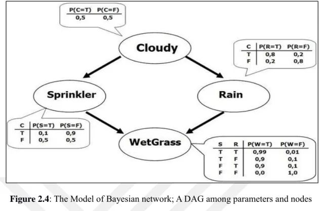
P (X1,…, Xn)=∏^𝑛_𝑖=1𝑃 (𝑋𝑖|𝑃𝑎(𝑋𝑖)) Equation 2-15 It needs to validate the Markov condition (definition 2). Fig. 2.4 gives an example of a BN representing the conditional relationships among four variables.

Def. 2. (Markov Condition): The BN of G = (V, E) indicated by M if every element in V is independent of every group of non-descendant elements given its ancestors.

(X⊥Non Descendent (X) | Pa(X)) Equation 2-16 Def. 3. (Faithfulness): P is a probability distribution, and M is the Bayesian network model is dedicated from one another if each of the independence connections correct within P is the needed through the Markov theory upon M [46].

Figure 2.4: The Model of Bayesian network; A DAG among parameters and nodes describing the probability distribution.

2.3.3 SOME PRINCIPLES OF BAYESIAN NETWORKS 2.3.3.1 D-SEPARATION GISRSMAMMAR@

To understand the flow of probabilistic control in the graph, we have to recognize how information moves from A into B to change the knowledge of C. Suppose three nodes are A, B and C, and also there is a route A—C—B. If the control flows from A to B via C so we can assume that the route A — C — B is active if it's not blocked [47]. It has three modes:

Serial relationship: If C is not detected then the route from A to B shall be active it shall be blocked. Within this situation we have, A⊥B |C and A⏈B.

Figure 2.5: Head-to-tail or Serial relation

Converging link: If C is not detected or it should block each descendant of C we have, A⏈B |C and A⊥B. This is also called V — structure.

A

A C B

C B

Figure 2.6: Head-to-head or Converging relation

Diverging link: If C not detected then the route on A to B will be open in the other case it would be blocked. So we have A⊥B |C and A⏈B.

Figure 2.7: Tail-to-tail connection or Diverging

Def. 4. Directional separation (D-separation). Assume A, B are arbitrary variables also C is a collection of arbitrary variables, A plus B is d-separated through C if and only if C blocks each route of A to B [48].

2.3.3.2 MARKOV EQUIVALENT CLASS

G1& G2 are Two DAGs said to be Markov equivalent if both provide the equivalent conditional independencies. This means that the DAGs which have equal d-separation are Markov equivalent. It means d-separation are Markov equivalent if all DAGs share the same one based on Verma and Pearl’s theorem:

Theorem 1. (Verma and Pearl: [49]) A Pair of DAGs (PDAG) are similar if and only if both own the equivalent frame also v-structures (head-to-head joint).

As an instance in Figure 2.8, there are four separate DAGs by the equal number of variables, and owning equal frames. According to Theorem 1, regular Markov equivalent classes are DAGs (a), (b) and (c). However, the v-structure A→C←B in (d), and it is just a graph under its equivalence class [50].

A B

C

A B

C

Figure 2.8: An example of Markov equivalent class, A, B, C, and

four DAGs. The (a), (b) and (c) DAGs have a similar independence structure while (d) compares to a different set of independencies.

2.3.4 QUERYING A DISTRIBUTION

The P(V) is the Bayesian network standard description of a complete mutual probability distribution. It can utilised while explaining probabilistic queries regarding the subgroup from unperceived variables while it perceives other variables. A simple query model holds the conditional probability query. In this query model, the query requested for a mutual distribution including the goal is to estimate [47]:

𝑃(𝑉|𝐸 = 𝑒) =^{𝑝(𝑉,𝑒)}_𝑃(𝑒) Equation 2-17 The equation 2-17 holds two parts,

– Variables (V) of the Query, V in the network is a subsection of arbitrary variables.

– Evidence (E), a subgroup from arbitrary variables within a pattern also the instantiation e

An extra query model is the maximum a posteriori probability (MAP). That calculates various responses to each of the variables if its non-evidence. [51]. If V and E are a collection to query variables and evidence in sequence, then.:

A

C

B A B

C

A

C

B

C

A B

a b

c d

MAP(V|e) arm𝑚𝑎𝑥_𝑋𝑃(𝑉, 𝑒) Equation 2-18

It allows calculating the posterior distribution of variables by probabilistic inference [52], also confirmed NP-hard [40]. Several methods introduced within an article in probabilistic inference. It separates these algorithms within exact inference procedures, plus approximate inference procedures — the comprehensive review of inference methods presented in Guo and Hsu [53].

2.3.4.1 EXACT INFERENCE

Pearl proposed a method for Bayesian Network tree-structure called the message propagation inference in [39]. The mentioned technique is a specific inference that also owns polynomial time complexity for all of the vertices. A different modern exact inference holds a joining tree or clique tree [54]. That recognized a clustering algorithm. The difficulty of the size from the biggest clique of the joining tree is exponential. Variable exclusion [55] stands further the Bayesian network exact inference algorithm. That reduces one by one of the variables through clearance out them. The number of mathematical multiplications and numerical summations it effects can adjust its complexity.

2.3.4.2 APPROXIMATE INFERENCE

Approximate inference algorithms are applied for complex structure more commonly than the exact inference. It depends on approximate inference methods of the Monte Carlo approaches. They produce the collection to pick random samples depending on the conditional probability tables within a form, approximate probabilities from query variables through repetitions from representation in the unit. Efficiency is base on the proportion of samples to represent the network structure [53]. A complexity of producing a unit also depends on network size.[56]. However, a problem among these algorithms is associated with a variety of the computed answers.

The primary method which utilises Monte Carlo approaches is logic sampling produced in [57]. Any of the other methods are holding probability weighting [58, 59], self-consequence sampling [59], heuristic interest [59], adaptive consequence sampling [41] etc.

2.4 BAYESIAN NETWORK LEARNING

In BNs, model picking and evaluation identified as learning, a title which acquired from machine learning and artificial intelligence. BN learning implemented as two procedures:

1. Structure learning: learning structure of the DAG;

2. Parameter learning: A local distribution for structured learning of DAG corresponding to the BN, using the data.

Learning can implement in two steps; as unsupervised learning, applying the information presented through a data set, or as supervised learning. Joining both procedures is the normal approach. Usually, the previous information accessible on the network is not suitable for an authority to define a BN. Furthermore, identifying the DAG structure is difficult, if it involves many variables. That is the case, for example, in gene network interpretation.

The following workflow is Bayesian. Assume a data set D and a BN, B = (G, V). If we show the parameters of the global distribution of V with Θ, we can suppose using externally available information that Θ recognizes V in the parametric group of populations for modelling D and write B = (G, Θ). BN learning can then formalized as

Pr(B | D) = Pr(G, Θ | D) = Pr(G | D). Pr(Θ | G, D) Equation 2-19

The breakdown of Pr(G, Θ | D) shows the steps described above and holds the logic of the learning procedure. Structure learning can accomplish by searching the DAG, G that maximizes:

Pr(G | D) ∝ Pr(G) Pr(D | G) = Pr(G)∫ Pr(D | G, Θ) Pr(Θ | G)dΘ Equation 2-20 Disintegrate the posterior probability of the DAG by applying the Bayes theorem (i.e., Pr(G | D)) within the result of the previous distribution across the potential DAGs (i.e., Pr(G)) also the possibility of using the data (i.e., Pr(D | G)). Obviously, It is not probable to calculate the latter externally, including determining the parameters Θ of G [60].

learning structure learning parameter learning

The prior distribution Pr(G) produces an excellent plan to introduce any prior information possible on the conditional independence associations among the variables in V. For example; we want that some arcs should exist within or missing from the DAG, to estimate to the penetrations achieved. It may also have needed that some arcs, if present in the DAG, must locate specifically if this way is the exclusive one that makes sense under the light of the logic defining the appearance of the standing model.

The usual regular selection for Pr(G) is a non-informative prior to the space of the DAGs, allowing the equivalent possibility to all DAG. It may refuse any DAGs for prior information, as explained before. Furthermore, complex priors (known as structural priors) are more probable, just unusually used in practice for a pair [60].

First, applying a normal probability distribution renders Pr(G) unnecessary in maximizing Pr (G | D). It makes it suitable for both computational and algebraic reasons. Second, the number regarding potential DAGs rises the number of nodes exponentially.

Defining a prior distribution across such a huge number of DAGs is a challenging responsibility for regular small problems.

Calculating Pr(D|G) is similarly uncertain from both an algebraic and computational point of representation. Beginning of the breakdown within local distributions, we can advance by factors of Pr(D|G) in the following way: [60]

Pr(D|G)=∫ ∏^𝑝_𝑖=1[Pr(𝑋_𝑖|Π_𝑋𝑖, Θ_𝑋𝑖) Pr(Θ_𝑋𝑖|Π_𝑋𝑖)]dΘ

= ∏^𝑝_𝑖=1[∫ Pr(𝑋𝑖|Π_𝑋𝑖, Θ_𝑋𝑖) Pr (Θ_𝑋𝑖|Π_𝑋𝑖)dΘ_𝑥𝑖]=∏^𝑝_𝑖=1𝐸_Θ𝑋𝑖[Pr (𝑋_𝑖|Π_𝑋𝑖] Equation 2-21

Using this form, Pr(D|G) can be calculated in a sensible time also for massive datasets.

This is reasonable both to the multinomial distribution considered for discrete BNs (via its conjugate Dirichlet posterior) and for the multivariate Gaussian distribution considered for continuous BNs (via its conjugate Inverse Wishart distribution). For discrete BNs, we can determine, Pr(D | G) in a Bayesian Dirichlet equivalent uniform (BDeu) score from [61]. Because it is the unique fragment of the BDe group of scores in normal usage, it is referred to as BDe.

BDe allows a flat score both over the parameter field of each node and the period of the DAGs:

Pr(G) ∝ 1 and Pr(ΘXi | ΠXi) = αij = _|Θ^α

𝑋𝑖| Equation 2-22

The exclusive parameter of BDe is the perfect representation size α compared among the Dirichlet prior, which concludes how much power it allocates to the prior as the size of an ideal description maintaining it. Following these hypotheses, BDe uses the following form [60]:

BDe(G,D)=∏^𝑝_𝑖=1𝐵𝐷𝑒(Xi, ΠXi)=∏ ∏ {Γ(αij + nij)^Γ(αij) ∏ Γ(αij + nijk) Γ(αijk)

𝑟𝑖𝑘=1 }

𝑞𝑖 𝑗=1 𝑝

𝑖=1 Equation 2-23

where:

• p is the number of nodes in G;

• ri is the number of classes concerning node Xi;

• qi is the number of arrangements from the categories of Xi's parents;

• nijk is the number for individuals who have the jth class for node Xi and the kth arrangement for its parents.

It names the similar posterior probability to GBNs Bayesian Gaussian equivalent uniform (BGeu) from [62], which again commonly referred to as BGe. Likewise, to BDe, it implies a noninformative prior to both the parameter range of every node also the range of the DAGs; and its only parameter is the ideal representation size α. Its definition is complicated, and will not be described here.

As a result of the problems described above, two options on the Pr(D|G) have been defined [60]. The first one is the use of the Bayesian Information Criterion (BIC) as an estimate of Pr (D | G), as

BIC (G, D) → log BDe (G, D) as the sample size n → ∞. Equation 2-24 BIC is analyzable and just based on the probability function,

BIC(G,D) =∑^𝑝_𝑖=1[log Pr(𝑋_𝑖|Π_𝑋𝑖) −^|Θ₂^𝑋𝑖|log 𝑛] Equation 2-25 Which, is relatively simple to calculate. The other option is to circumvent the requirement to establish a standard of goodness-of-fit to the DAG also to apply

conditional independence experiments for learning the DAG structure individual arc in time [60].

Once become learned the DAG structure can drive to parameter learning, for which we can determine the parameters for the set of nodes X. Considering that parameters relating to various local distributions are independent, really require determining just the parameters of individual local distributions in time. Following the Bayesian procedure described in Equation (2-19), this would need to get the value of the Θ which maximizes Pr (Θ|G, D) by its elements Pr (ΘXi|Xi, ΠXi). Additional approaches to parameter estimation exist, such as the highest likelihood regularized evaluation.

Local distributions in tradition require just a small number of nodes, i.e., Xi and its parents ΠXi. Their dimension regularly does not balance among the number of nodes in the BN (and often considered being limited by a fixed number of nodes while determining the computational complexity of algorithms), therefore circumventing the nominal curse of dimensionality. That shows every local distribution owns the relatively few numbers from parameters for the test individually and also that estimates are specific in greater proportion within a size from ΘXi plus a sample size.

2.4.1 LEARNING THE STRUCTURE OF BAYESIAN NETWORKS

Suppose the following circumstances. Any means provide representations of states of a candidate BN (N) across the universe U, and the required building the BN of a problem. It is a common framework for Bayesian networks structural learning.

Meanwhile, the actual environment unable to sure that can test the states of the network, but we will consider this case. Also, consider the sample is appropriate, and a set D from states shows a distribution PN(U) which enable via N.

We think all connections within N are required; for example, if the connection is released, then a network producing unable to express P(U). It can explain as arises: if parents of X are pa(X) are, also Y represents each concerning them, next there are a couple of cases x1 and x2 of Y and an arrangement z of the different parents so that

P (X|x1, Z) ≠ P (X|x2, Z).

To get an M, near to N in Bayesian network, can be accomplished through operating learning parameter during every potential structure also picking those types to which

PM(U) near to (U). Aforementioned straightforward procedure challenged among three difficulties, that are necessary for Bayesian networks learning. First, the area from every Bayesian network structure is significant. In reality, the amount from various structures, f(n), raises even larger to exponentially during the amount of nodes n it can get (recent case estimations give in Table2.1):

𝑓(𝑛) = ∑^𝑛_𝑖=1(−1)^𝑖+1_{(𝑛−𝑖)! 𝑛!} ^𝑛! 2^{𝑖(𝑛−𝑖)}𝑓(𝑛 − 1) Equation 2-26

Second, while seeking within the network structures, we may finish up by some uniformly excellent structures candidate. For over a whole graph in Bayesian network able to describe each configuration covering its universe, we comprehend that it will regularly own some candidates, although a BN over a comprehensive graph will barely be the accurate solution. If so, it is a limited solution.

Third, it has a difficulty from over-fitting: a picked model is so familiar to 𝑃_𝐷^#(U) least aberrations of PN(U), over, the comprehensive graph can describe (U) correctly, still, D may have inspected an incompetent system. It has two approaches applied for Bayesian networks structure learning; score-based plus constraint-based. A score- based approach provides a sequence of applicant Bayesian networks, compute a score during all applicant, also declare an applicant of the most significant score. The

Table 2.1. The table presents the amount of various DAGs that can produce several nodes. For example, there are 1.4*10⁴¹ different DAGs with 14 nodes.

NODES Number of DAG NODES Number of DAG

1 1 8 7.8*10¹¹

2 3 9 1.2*10¹⁵

3 35 10 4.2*10¹⁸

4 543 11 3.2*10²²

5 29281 12 5.2*10²⁶

6 3.8*10⁶ 13 1.9*10³¹

7 1.1*10⁹ 14 1.4*10⁴¹

constraint-based approaches organize a collection of conditional independence observations, including the data plus apply the set to construct a network among d- separation attributes comparing the conditional restricted independence properties.

To show a centre of structural learning, it should apply these following rule: A Bayesian network M = (S, θS) composed of the structured network, S, plus a collection of parameters, θS, where the conditional probabilities of the model defined by parameters. The S is a structure composed of a DAG, G = (U, E), mutually among a designation of the event period for every node per variable within a graph.

2.4.1.1 THE SCHEMA FOR LEARNING STRUCTURE

All DAG that contains the same node can be disjoint in the equivalence classes by Markov equivalence; also all DAG that produced Markov Equivalence class has equal distribution probability. Furthermore, the DAG pattern can build upon a graph called DAG that expresses the entire Markov equivalence class. We will use GP as a stochastic random variable whose potential values are DAG models, (gp). As far as they involve the genuine corresponding frequency distribution, a DAG model case (gp) is the case that (gp) is dedicated to the corresponding frequency distribution. In some circumstances, we may recognize DAG related problems. For instance, if an issue is a causal structure between the variables, then X1 → X2 expresses the case that X1 causes X2, while X2 → X1 describes the different events that X2 causes X1. But unless declared, only check DAG model issues, including the notation ρ|G confirms the quantity function in the developed Bayesian network including the DAG (G). It seems not to require that the DAG (G) is an issue.

We have the following explanation concerning learning structure:

Definition 6 The following makes up a multinomial Bayesian network structure learning schema:

1. n random variables X1, X2, ... Xn with mutual joint probability distribution P;

2. an equivalent representation size N;

3. for each DAG model (gp) including the n variables, a multinomial expanded Bayesian network (G, F(G), ρ|G) including equivalent sample size N, where G is any

part of the equivalence group expressed by (gp), such that P is the probability distribution in its secured Bayesian network.

Note that even though a Bayesian network containing the DAG X1 → X2 can include a configuration in which X1 and X2 are independent, the case (gp)1 is the case they conditioned also, does not allow the case they are independent. As usual, we do not immediately select a mutual probability distribution because the number of values in the mutual distribution increases exponentially with the number of variables.

Preferably we select dependent distributions from the expanded Bayesian networks such that the probability distributions in all the fixed Bayesian networks are equivalent.

For, a presented DAG model (gp), we first discover a DAG G in the equality group it represents. Then in the expanded Bayesian network corresponding to G for all i, j, and k we set: aijk =_{𝑟𝑖𝑞𝑖}^𝑁

where ri is the number of potential values of Xi in G, and qi is the number of various instantiations of the parents of Xi [61] presents other techniques for testing priors.

2.4.1.2 PROCEDURE FOR LEARNING STRUCTURE

This part displays how we can learn structure using a multinomial Bayesian network structure learning schema. We begin with this explanation:

Definition 7 The following forms a multinomial Bayesian network structure learning space:

1. a multinomial Bayesian network structure learning schema, including the variables X1, X2,… Xn;

2. A stochastic variable GP whose scope comprises every DAG models including the n variables, and for any value gp of GP a prior probability P(gp);

3. A set D = {X⁽¹⁾, X^(2), ... X^(M)} of n-dimensional arbitrary vectors such that every 𝑋_𝑖^(ℎ) has the equivalent space as Xi for any value gp of GP, D is a multinomial Bayesian network sample of size M with parameter (G, F^(G)), where (G, F^(G)) is the multinomial expanded Bayesian network comparing to gp in the schema's specification.

A scoring model for a DAG (or DAG model) is a role that selects a meaning to each DAG (or DAG model) depend on consideration based on the data. The formulation in