Parameter Quantization Effects in Gaussian Potential Function Neural Networks

Parameter Quantization Effects in

Gaussian Potential Function Neural Networks

ERKAN KARAKUŞ

(1)

, ARİF SELÇUK ÖĞRENCİ

(2)

, GÜNHAN DÜNDAR

(1)

(1)

_{Department of Electrical and Electronics Engineering}

Boğaziçi University

80815-Bebek, Istanbul

TURKEY

(2)

_{Department of Electronics Engineering}

Kadir Has University

Vefabey Sok. 5, 80810-Gayrettepe, Istanbul

TURKEY

Abstract: - In hardware implementations of Gaussian Potential Function Neural Networks (GPFNN), deviation

from ideal network parameters is inevitable because of the techniques used for parameter storage and implementation of the functions electronically, resulting in loss of accuracy. This loss in accuracy can be represented by quantization of the network parameters. In order to predict this effect, theoretical approaches are proposed. One-input, one-output GPFNN with one hidden layer have been trained as function approximators using the Gradient Descent algorithm. After the training, the network parameters (means and standard deviations of the hidden units and the connection weights) are quantized up to 16-bits in order to observe the percentage error on network output stemming from parameter quantization. Simulation results are compared with the predictions of the theoretical approach. Consequently, the behaviour of the network output has been given with combined and separate parameter quantizations. Moreover, given the allowed percentage error for the network, a method is proposed where the minimum number of bits required for quantization of each parameter could be determined based on the theoretical predictions.

Key-Words: - Gaussian potential function neural networks, weight quantization, training.

1 Introduction

One of the challenging problems encountered in the design of neural network circuitry is the storage of parameters. Due to the techniques used for parameter storage such as digital memories, capacitors, and transistors, deviation from ideal network parameters is inevitable. As an example, quantization of ideal network parameters for easier storage may lead to a remarkable level of inaccuracy in hardware implementation of neural networks. Learning algorithms that are efficiently implemented on general-purpose digital computers encounter great difficulties while mapped onto VLSI hardware: deviations of parameters may significantly affect the performance of the trained system unless the more costly “chip in the loop” training is performed. A serious problem here is to predict the upper bound of inaccuracy to ensure a certain performance during the training stage. The remedy is to investigate the parameter quantization effects on neural network output and to provide an analytic solution based on

probabilistic analysis for prediction of these effects. Such an analysis for multilayer perceptron neural networks has been carried out by several researchers [1, 2]. In this work, parameter quantization effects will be investigated and predicted for GPFNN. GPFNN are considered in virtue of their wide usage for both supervised and unsupervised types of learning. They are used for function approximation where the highly nonlinear Gaussian basis functions provide good locality for incremental learning. GPFNN are also used where a similarity measure has to be computed such as in classification and self-organization problems. Section 2 investigates the parameter quantization effects for a specific network, and a theoretical approach based on a probabilistic analysis is provided in order to predict network error resulting from parameter quantization. Next, results obtained for both experimental and theoretical methods are given where the network parameters (mean and standard deviation parameters of Gaussian activation function and the weights on the

output synapses,) are quantized up to 16-bits to observe the network performance. In the conclusion, results are summarized and an optimization method is proposed, in which, given the percentage error, the optimum number of bits for each parameter quantization is found using the predictions of the theoretical approach.

2 The Effects of Neural Network

Parameter Quantization

A single input - single output Gaussian Potential Function Network (GPFN) is considered for the analysis of parameter quantization on network performance. The Gradient Descent algorithm is used to train the network as a function approximator. After the training, the network parameters (which are the means and standard deviations of the hidden units and the connection weights) are quantized to observe the error on network output stemming from parameter quantization. This is performed separately on all parameters first, then together. Then, theoretical and experimental percentage error (PE) on the output is calculated for each parameters quantization. For this purpose, a theoretical approach will be derived to predict the network error resulting from parameter quantization.

In the following, 0

1

x is the input to the neural

network, 0

i

y is the input to each hidden unit, 1

i

x is the

output of each hidden unit, w are the weights, y1_{is the}

output of the neural network. The weights on the synapses connecting the input node to hidden nodes are equal to one, hence

0 1 0 _x y_i = (1)

( )

y m s e y f x i i i i i 2 2 0 0 1_{= =} − −  ₍₂₎

Then, the network output is,

∑

− = = 1 0 1 1 1 N i i i x w y (3)

The experimental percentage error calculation will be carried out by the following formula,

signal noise PE σ σ = (4)

where _σnoise is the standard deviation of the

quantization error which is considered as a noise on desired signals.

In the following sections, derivation of the standard deviation of the error and of the desired output will be given for each parameter perturbation of the network, namely the mean, standard deviation, and weights.

2.1 Weight Quantization Effects

The weight values are assumed to have a uniform distribution between -max(w) and max(w) where

max(w) is the maximum weight value obtained from

simulation results [1, 2]. Distribution parameters of connection weights are found as follows [2]:

0 = w m (5) 3 ) max( . ) max( 2 1 max( ) 2 ) max( 2 2 _{w dw} w w w w w =

∫

= − σ (6)

The weight quantization effect on the network output can be expressed by the following:

(

)

∑

− = +∆ = 1 0 1 1 1 1 N i i i i x w w y (7)

and the error on the network output becomes,

∑

− = ∆ = ∆ 1 0 1 1 1 N i i i x w y (8)

where ∆w_i1is the quantization error (noise) of the

weights. Quantization error has a uniform probability

distribution between -∆_w/2 and +∆_w/2

where 1 2 2 _max − = ∆w _B w

is the quantization increment

with wmax being the upper bound of the quantization

interval and B is the number of bits used in quantization. The distribution parameters of quantization error are found as follows [2]:

0 = ∆w m (9) 12 1 2 2 2 2 2 w w w w w d∆=∆ ∆ ∆ =

_∫

∆ ∆ − ∆ σ (10)

The variance of the error in network output is

( ) ( )

∑

( )

( )

∑

−

( )

= − = + ∆ ∆ = ∆ 1 0 1 2 1 0 2 1 N i i N i i x V w E x E w V y V (11)

Since E

( )

∆w =0, the variance of the error becomes,

( ) ( )

∑

−

( )

= ∆ = ∆ 1 0 2 1 N i i x E w V y V (12)

Similarly, variance of the actual network output is,

( )

( )

∑

( )

( )

∑

−

( )

= − = + = 1 0 1 2 1 0 2 1 1 N i i N i i real V w E x E w V x y V (13) Since E

( )

w =0, then

( )

( )

∑

−

( )

= = 1 0 2 1 1 N i i real V w E x y V (14)

The percentage error due to weight quantization can be expressed as

( )

( )

V

( )

( )

w w V y V y V PE real w = ∆₁ = ∆ ) ( (15)

and using (6) and (10), PE is found as follows:

( )

.

( )

2 1 max ) ( max − = _B w w w PE (16)

2.2 Mean Value Quantization Effects

The input of the network is assumed to be time, varying in the interval [0, 2L], where 2L is the period in which the function is to be approximated by the neural network. Hence, it is conceivable that the network input and mean values of the hidden units will have a uniform probability distribution between 0 and 2L (this assertion will be modified in Section 3, in order to get an upper bound estimate for the quantization effect): mean and standard deviation of the network input and mean (center values) above can easily be found as:

L m m_x0 = m = 1 (17)

(

)

₃ 2 1 2 2 0 2 2 2 0 1 L dm L m L L m x =σ =

∫

− = σ (18)

and distribution parameters of quantization error,

m

∆ , are similar to those of∆w.

In order to eliminate the exponential term in the Gaussian activation function for easier mathematical

manipulation, Taylor series expansion of _ea _around

a=0 will be used, then the activation function

becomes

( ) (

) (

4

)

4 0 2 2 0 0 2 1 i i i i i i i s m y s m y y f = − − + − (19)

The mean quantization effect on the network output can be expressed in the following form:

(

)

∑

− = +∆ = 1 0 1 N _. i i i i x x w y (20)

Finally one finds the error in the network output as:

(

)

(

)

∑− =                           ₋ −     ₋ + −     _{− +∆} +     _{− +∆} − = ∆ 1 0 4 2 4 0 2 2 0 1 4 2 4 0 2 2 0 1 1 N i i s i m i y i s i m i y i s i m i m i y i s i m i m i y wi y (21)

Variance of a function of n independent random variables, say Z =H

(

X₁,...,X_n

)

with E

( )

X_i =µ_i and

( )

2

i i

X

V =σ , is given by the following:

( )

∑

=      ∂ ∂ ≈ n i Xi i H Z V 1 2 2 σ (22) where all the partial derivatives are evaluated at the

point

(

µ₁,...,µ_n

)

. By applying (22), the standard

deviation of the error becomes,

( )

1 . 2₂

( ) ( )

2₄ 3 . ₁₂ 1 m y L m s m L s w N y V ∆         − − − = ∆ = ∆ σ (23)

where parameters with overbars indicate the variables’ expected values. In Section 3, it will be shown how to determine the expected values.

According to (14),

( )

1

i

x

E is required to be

calculated in order to find the variance of the output obtained without parameter quantization. The

expected value of hidden unit output,

( )

1

i

x

E , is found

according to the approach derived in [2]. First, the cumulative distribution function for x is derived. Then the pdf of x is found and the expected value of

x becomes,

[ ]

dx x L s x E

_∫

− = 1 0 ln 1 4 (24)

After some mathematical manipulation this yields

[ ]

x s _L E

4

π

= (25)

Then, substituting (25) into (14), the standard deviation of the output becomes,

∑

− =         = 1 0 2 4 1 N i i w y _L s real π σ σ (26)

Finally, by substituting (26) into (4), percentage error (PE) is found as follows,

( ) ( )

∑

− =                 − − − ∆ = 1 0 2 3 4 2 4 . 1 1 . 3 ) ( N i i w m m L s m L s m L s w N PE π σ (27)

2.3 Quantization Effects of Standard

Deviation

Similar to mean quantization, quantization effect of standard deviation on the network output can be expressed in (16) and distribution parameters of

quantization error, ∆sare similar to those of ∆w.

By using the Taylor approximation, error on the network output can be expressed by,

(

) (

)

(

)

(

)

(

)

(

)

∑

− =                 − − ∆ + − + ∆ + − − − = ∆ 1 0 4 4 0 4 4 0 2 2 0 2 2 0 1 2 . 2 N i i i i i i i i i i i i i i i i s m y s s m y s s m y s m y w y (28)

and by applying (22), the standard deviation of error on the network output is found as,

( )

1 . 2₃

( )

2 2₅

( )

4 . ₁₂ 1 s y L m s m L s w N y V _ ∆       − − − = ∆ = ∆ σ (29)

Finally, by substituting the equations (26) and (29) into (4), percentage error (PE) is found as follows,

( )

( )

∑

− =                 − − − ∆ = 1 0 2 4 5 2 3 4 . 1 1 . 3 ) ( N i i w s s L s m L s m L s w N PE π σ (30)

When all parameters, mean, standard deviation and weights, are quantized together, each quantization will contribute to the error on the network independent of each other [1]. Hence, a worst case (upper bound) estimate of the percentage error caused by quantization of all parameters will be the sum of percentage errors caused by quantization of each parameter:

( ) ( ) ( )

PE w PE m PE s

PE≤ + + (31)

3 Simulation Experiments

After having derived the theoretical methods for the prediction of network parameter quantization effects, comparison of the theoretical results to the simulation results will be presented. The GPFNN used in the simulation has been trained as a function approximator. Simulations are carried out for several

periodic (sin(x), sin(x)*cos(x), etc. over [0,2_{π]) and}

non-periodic functions

(f(x)=x(x-1)(x-1.5)(x-2.5)(x-3) over [0,3]) for different numbers of hidden units.

In the following, results for sin(x)*cos(x) and for the polynomial with N=14 hidden units are given. The neural networks are trained by software using 32-bit precision for a rms error of less than 0.1%.

3.1 Results for sin(x)*cos(x)

:

For the theoretical results, two different approaches will be used for the function sin(x)*cos(x) (and similar periodic functions). In the following, the expected values for the parameters, weight and mean, obtained from (5) and (17) will not be directly

used for the terms w and m, since this will cause

(27) and (30) to be equal to zero. It is obvious that this would happen if all the Gaussians were identical to each other and equally spaced. Instead, they will

be evaluated on two different sets for the terms, w,

m and s in order to compute the upper bound for

the possible percentage error. In the first approach,

the terms w and s are directly evaluated from the

training results as s =mean(s) and w=mean(w) where

) (s

mean and mean(w) are the arithmetical mean of

standard deviation and center values of hidden units

obtained from simulation results. m is chosen as

follows: Assume that the interval of interest is covered by N Gaussians in such a way that the center

of each one coincides with its neighbouring

Gaussian’s tail at the level of only 1/e2_{≈ 10% of the}

neighbour’s maximum. Hence, the maximum distance between the centers of two Gaussians

becomes s 2 . Therefore, the maximum deviation of

the average of the centers can be taken as s 2,

implying that

2

s

m=π # (32)

This value of malso agrees well with the average of

the centers obtained from simulations, mean(m).

Substituting (32) into (27) and (30) yields,

( )

( )

_∑

− =         ∆ = 1 0 2 4 3 max 2 . . . 3 N i i m m L s w s w N PE π (33)

( )

( )

_∑

− =         ∆ = 1 0 2 4 3 max 2 . . . 3 N i i s s L s w s w N PE π (34)

In the second approach, w and s are chosen

empirically. From several simulation runs with employing different number of hidden units, it has been observed that

N w w 25 ) max( = (35)

Intiutively, s should also be given by the formula

N L k

s= (36) where k is a measure of the “complexity” of the problem. As the function exhibits more fluctuations, i.e. becomes more “complex”, the standard deviations of the Gaussians have to be smaller for attaining the required locality and preserving the generalization ability of GPFNN. For the function

sin(x), k=2/3 and for sin(x)cos(x), k=1/2. Finally, m

is calculated as given by (32).

3.2 Results for the polynomial

The polynomial f(x)=x(x-1)(x-1.5)(x-2.5)(x-3) is not symmetrical with respect to any point in[0,3]. It also has a non-zero average value, thus, the expected value of the weight values will not be zero. Then it becomes necessary to consider the variance of the hidden units’ outputs in (14). We can assume, however, that the weight values are uniformly distributed between the maximum weight value,

max(w), and the minimum weight value, min(w),

distribution parameters of connection weights are found as follows: 2 ) max( ) min(w w mw = + (37)

(

)

12 ) min( ) max( 2 2 w w w= − σ (38)

Using (12) and (14) percentage error for weight quantization can be expressed as

∑

∑

∑

− = − = − = + ∆ = ₁ 0 2 1 0 2 1 0 2 ) ( ) ( ) ( ) ( ) ( ) ( ) ( N i l i N i l i N i l i w x V w E x E w V x E w V PE (39)

Since E(w)_{≠0, the variance of hidden units’ output,}

V(x), has to be calculated to be used in (39):

dx x E e x V b a m y 2 2 ) ( ) ( ) ( 2 2

∫

_       − = − − σ ₍₄₀₎

where a and b are the lower and upper bounds of the interval of the function respectively. For our problem, this is obtained after some mathematical manipulation as

(

)

(

)

( ) 4 2 ) ( ) ( 2 ) 2 ( ) 2 ( ) ( 2 2 2 1 2 2 1 2 a b L x erf x erf L x erf x erf s x V − + − − − = πσ πσ π (41) where x2 =(b−m)/σ, x1=(a−m)/σ, and 2 / ) ( 2 b a

L = + . The percentage error for the mean

value and standard deviation quantization can be

found similar to (33) and (34) where w, m and

sare computed using the two approaches as in the

previous example.

( )

(

)

₍

₎

∑

∑

− = − = +         − − − ∆ = 1 0 2 1 0 2 2 2 2 2 2 ) ( ) ( ) ( ) ( 1 1 . . 3 N i l i N i l i m m x V w E x E w V m L s s m L w N PE (42)

( )

( )

_{( )}

∑

∑

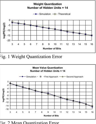
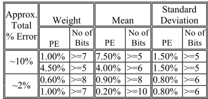
− = − = +         − − − ∆ = ₁ 0 2 1 0 2 2 2 3 2 ) ( ) ( ) ( ) ( 1 1 . . 3 N i l i N i l i s s x V w E x E w V m s s m w N PE π π (43) In the next column, effects of parameter quantization are given as the graph of the “percentage error” versus the “number of bits used”, in logarithmic scale for the sin(x)*cos(x) problem. For mean and standard deviation quantization, both theoretical approaches are compared to the simulation results. During the simulations, first, each parameter of interest is quantized separately (Figures 1, 2, 3.) Then, all parameters are quantized in Fig. 4.

All graphs displayed exponential behaviour, that is why a normalized logarithmic scale is used.

Weight Quantization Number of Hidden Units = 14

-20 -15 -10 -5 0 3 4 5 6 7 8 9 10 11 12 13 14 15 16 Number of Bits log(PE)/log(2) Simulation Theoretical

Fig. 1 Weight Quantization Error

Mean Value Quantization Number of Hidden Units = 14

-16 -14 -12 -10 -8 -6 -4 -2 0 3 4 5 6 7 8 9 10 11 12 13 14 15 16 Number of Bits log(PE)/log(2)

Simulation First Approach Second Approach

Fig. 2 Mean Quantization Error

Standard-Deviation Quantization Number of Hidden Units = 14

-18 -16 -14 -12 -10 -8 -6 -4 -2 0 3 4 5 6 7 8 9 10 11 12 13 14 15 16 Number of Bits log(PE)/log(2)

Simulation First Approach Second Approach

Fig. 3 Standard Deviation Quantization Error

Weight-Mean-Std. Dev Quantization Number of Hidden Units = 14

-16 -14 -12 -10 -8 -6 -4 -2 0 3 4 5 6 7 8 9 10 11 12 13 14 15 16 Number of Bits log(PE)/log(2)

Simulation First Approach Second Approach

Fig. 4 Weight-Mean-Standard Deviation Quantization Error

4 Results and Conclusion

In this work, the GPFN was trained with the Gradient Descent algorithm for several different function approximation examples. In order to observe the network performance affected by parameter quantization, network parameters, which are the connection weights, means and standard deviation of hidden units, were disturbed with up to 16-bit quantization noise. This was performed on all parameters first separately, then together and it was observed that the performance of the resultant network was degraded by quantization noise and showed an exponential dependence on resolution. The same bahaviour has also been reported in [2] for multilayer perceptron neural networks.

Two theoretical approaches are derived in order to predict the behaviour of network performance affected by parameter quantization noise based on statistical analysis of network parameters. Both approaches for theoretical predictions almost coincided. This indicates that the estimation proposed for the placement of Gaussian hiddens for the functions is in accordance with the real case. It was also seen that both theoretical approaches agreed well with simulations. It has been also shown in the simulations that the network performance exhibits exponential dependence on resolution and was degraded with decreasing resolution.

It was observed that quantization noise on connection weights and means of the hidden units plays an important role on network performance. The performance was satisfactory only with 8 or greater of number of bits quantization on these parameters. On the other hand, the network performance did not degrade markedly with standard deviation quantization as compared to other parameter quantizations. Similar precision requirements are also reported in [3].

Given the required percentage error of the network, minimum number of bits for each parameter quantization can be determined based on the theoretical results. Table 1 shows an example of such determination based on the results of second theoretical approach obtained by training the network. As can be seen from Table 1, to provide the required performance, the minimum number of bits per parameter quantization can be determined in several ways. For instance, to ensure a percentage error of 2 per cent, while one set of quantization bits would be {8,8,6}, the other one would be {7,10,6}. Moreover, an optimization could be applied to the following cost function that takes the hardware area cost for each parameter into account.

Cost= k1Bw+k2Bm+k3Bs (44)

where k1, k2, and k3 are the area requirements for

each weight that may depend on the implementation style. By minimizing the cost, optimum number of bits for each parameter can be found. As an example, the area requirement per bit for each parameter is the same in a DAC (Digital to Analog Converter) style parameter storage system. Hence the cost to be minimized is simply the sum of the bit counts for the parameters [4].

The main outcomes of the approach here can be stated as follows: time can be saved for predicting the effects of quantization by employing the semi-analytic approach. These results can be used in designing the architecture of the hardware. Furthermore, these results give some insight on how the quantization of the parameters affect the overall behaviour of the network. However, small modifications are necessary depending on the characteristics of the function to be approximated. As a future study, the techniques developed for predicting the network error against parameter quantization in approximation problem could be extended to other kinds of problems.

Table 1 Determination of minimum number of bits per parameter for a given percentage error for sin(x).

References:

[1] Xie, Y. and M.A. Jabri, “Analysis of the Effects of Quantization in Multilayer Neural Networks Using a Statistical Model,” IEEE Trans. on

Neural Networks, Vol. 3, No: 2, 1992.

[2] Dündar, G. and K. Rose, “The Effects of

Quantization on Multilayer Neural Networks,”

IEEE Trans. on Neural Networks, Vol. 6, No: 6,

1995, pp. 1446-1451.

[3] Murray, A. and L. Tarassenko, Pulse Stream VLSI for RBF Neural Networks, Final Report, http://www.ee.ed.ac.uk/~neural/research/RB Fproject/, 1999

[4] Çevikbaş, İ.C., A.S. Öğrenci, S. Balkır, and G. Dündar, “VLSI Implementation of GRBF Networks,” Proc. of ISCAS’2000, Geneve, May 2000. Weight Mean Standard Deviation Approx. Total % Error PE No of

Bits PE No of Bits PE No of Bits

1.00% >=7 7.50% >=5 1.50% >=5 ~10% 4.50% >=5 4.00% >=6 1.50% >=5 0.60% >=8 0.90% >=8 0.80% >=6 ~2% 1.00% >=7 0.20% >=10 0.80% >=6