Development of a vector sensor using piezoelectric support beams

DEVELOPMENT OF A VECTOR SENSOR

USING PIEZOELECTRIC SUPPORT BEAMS

a thesis submitted to

the graduate school of engineering and science

of bilkent university

in partial fulfillment of the requirements for

the degree of

master of science

in

mechanical engineering

By

Alper Yasin Tiftik¸ci

August 2016

DEVELOPMENT OF A VECTOR SENSOR USING PIEZOELEC-TRIC SUPPORT BEAMS

By Alper Yasin Tiftik¸ci August 2016

We certify that we have read this thesis and that in our opinion it is fully adequate, in scope and in quality, as a thesis for the degree of Master of Science.

Melih C¸ akmak¸cı(Advisor)

Yi˘git Karpat

Kutluk Bilge Arıkan

Approved for the Graduate School of Engineering and Science:

Prof. Dr. Levent Onural Director of the Graduate School

ABSTRACT

DEVELOPMENT OF A VECTOR SENSOR USING

PIEZOELECTRIC SUPPORT BEAMS

Alper Yasin Tiftik¸ci M.S. in Mechanical Engineering

Advisor: Melih C¸ akmak¸cı August 2016

Underwater listening has attracted great interest since the twentieth century. Formerly, scalar hydrophones were used to detect sounds underwater by measur-ing only the pressure changes. These sensors needed to form an array to detect the direction of an incoming wave. They were positioned with intervals and the time delays of the sound among hydrophones gave the information of direction. However, vector hydrophones have become an attractive alternative since they can provide both scalar and vector information on their own.

An Acoustic Vector Sensor (AVS) is a device used to detect acoustic signals by converting mechanical energy of an incident wave to a detectable electrical energy. Its design is based on two parallel piezoelectric beams attached to a mechanical sensing tip using a rotary joint component. The sensor uses piezoelectric elements to convert mechanical strain into sensible electrical signal. Design of the sensor is modular since each individual sensing element could be easily changed, tested and calibrated. All parts of sensor has been fabricated by mechanical micromachining and precisely assembled, which increases design and manufacturing flexibility.

In this thesis, the mechanical design of the sensor that uses the piezoelectric effect for detection of sound is presented. First, a computational analysis method which predicts the dynamic response of the designed sensor is developed. Then, a tigthly controlled vibration experiment platform is set up to emulate the effect of the motion of the acoustic particle. The computational simulations are then validated with initial experiments and the design of the sensor is finalized. Keywords: acoustic vector sensor, piezoelectric effect, finite element analyses, micro-fabrication.

¨

OZET

P˙IEZOELEKTR˙IK DESTEK K˙IR˙IS

¸LER˙I KULLANILAN

VEKT ¨

OR SENS ¨

OR GEL˙IS

¸T˙IR˙ILMES˙I

Alper Yasin Tiftik¸ci

Makine M¨uhendisli˘gi, Y¨uksek Lisans Tez Danı¸smanı: Melih C¸ akmak¸cı

A˘gustos 2016

Sualtı dinleme teknolojisi yirminci y¨uzyıldan beri ¸cok fazla ilgi g¨ormektedir. Daha ¨onceleri, sualtındaki sesleri belirlemek i¸cin sadece basın¸c de˘gi¸simlerini ¨ol¸cen skaler hidrofonlar kullanılıyordu. Bunların gelen dalganın y¨on¨un¨u belirleye-bilmeleri i¸cin bir dizin olu¸sturmaları gerekiyordu. Bu hidrofonlar belirli aralıklarla diziliyor ve sesin hidrofonlara ula¸smasındaki zaman farkı kullanılarak y¨on bilgisi elde ediliyordu. Bununla birlikte, vekt¨or hidrofonlar ilgi ¸cekici bir alternatif haline geldi ¸c¨unk¨u bu hidrofon tek ba¸sına hem skaler hem de vekt¨orel bilgi sa˘glayabiliyor. Akustik Vekt¨or Sens¨or (AVS) gelen sinyalin mekanik enerjisini ¨ol¸c¨ulebilen elek-trik enerjiye ¸ceviren bir cihazdır. Bir mekanik duyarlı ¸cubu˘ga ba˘glı iki paralel piezoelektrik kollara dayalı dizayn edilmi¸stir. Dizayn edilen sens¨orde, mekanik gerinimi ¨ol¸c¨ulebilir elektrik sinyaline ¸cevirmek i¸cin piezoelektrik elemanlar kul-lanılır. Sens¨or dizaynı mod¨uler olacak ¸sekilde kurgulanmı¸stır bunun nedeni par¸calar kolayca de˘gi¸stirilebilir, test edilebilir ve kalibre edilebilir. Sens¨or¨un b¨ut¨un par¸caları mekanik mikroi¸sleme teknikleri ile ¨uretilmi¸stir ve hassas bir bi¸cimde bir araya getirilmi¸stir, bu da dizayn ve ¨uretim konusunda esneklik sa˘glar. Bu tezde, sesin algılanması i¸cin piezoelektrik etkiyi kullanan sens¨or dizaynı sunulmaktadır. ˙Ilk olarak dizayn edilen sens¨or¨un dinamik cevabını ¨ong¨oren bir hesaplamalı analiz metodu geli¸stirilmi¸stir. ˙Iyi kontrol edilebilen bir salınım plat-formu kurulmu¸stur. Hesaplamalı sim¨ulasyonlar ilk deneylerle do˘grulanmı¸s ve sens¨or dizaynı sonlandırılmı¸stır.

Anahtar s¨ozc¨ukler : akustik vekt¨or sens¨or, piezoelektrik etki, sonlu elemanlar anal-izleri, mikro-¨uretim.

Acknowledgement

First of all, I would like to thank my advisor Assist. Prof. Melih C¸ akmak¸cı with all my sincerity for his support through all my graduate study. He directed and motivated me all the research period with his valuable advices. I will not forget his helps not only for research but also for my future life.

I would like to thank Prof. Dr. Adnan Akay and Assoc. Prof. Dr. Yi˘git Karpat for their contributions to this project. Their guidances were really helpful for developing this project.

I would like to thank Dr. S¸akir Baytaro˘glu for his helps in experimental studies and his advices. Also, I thank Mustafa Kılı¸c for his efforts in manufacturing process.

I thank my fellows Serhat Kerimo˘glu, Erkan Bu˘gra T¨ureyen, M¨umtazcan Karag¨oz, Samad Nadimi, Stefan Ristevski, Elif Altıntepe, Abdullah Waseem and the rest of all graduate students in our department for the great time we had in the last three years.

I would like to thank my family for their moral support in writing this thesis and for their unlimited support in my whole life.

Lastly, I would like to thank Meteksan Defense Industry for their financial and technical support throughout the end of the project. I would like to thank Ahmet Levent Av¸sar and Can Aksoy for their contributions to this project.

Contents

1 Introduction 1

1.1 Introduction . . . 1

1.2 Motivation and Contribution . . . 5

2 Design and Manufacturing 8 2.1 Theory . . . 8

2.2 Parts used in the Design . . . 9

2.2.1 Mechanical Sensing Tip . . . 12

2.2.2 Connection Mass . . . 12

2.2.3 PZT Beams . . . 13

2.2.4 Copper Plates . . . 13

2.2.5 Bases . . . 14

2.2.6 Metal Rods . . . 14

CONTENTS vii

2.4 Manufacturing and Assembly Procedure . . . 16

3 Modeling 19 3.1 Mathematical Formulation . . . 20

3.1.1 Maximum Deflection of a Rod Fixed at One End . . . 20

3.1.2 Natural Frequency of a Rod Fixed at One End . . . 22

3.2 Finite Element Analysis . . . 24

3.2.1 Vibration Modes and Natural Frequencies of AVS . . . 25

3.2.2 Frequency Response of AVS . . . 25

3.2.3 Directivity Pattern of AVS . . . 28

3.2.4 Model of AVS with Assembly Effects . . . 30

4 Experimental Setup and Experiments 39 4.1 Equipment Used in the Test Setup . . . 40

4.1.1 Vibration Controller . . . 40 4.1.2 Power Amplifier . . . 40 4.1.3 Electro-Dynamic Shaker . . . 42 4.1.4 Accelerometer . . . 42 4.1.5 Software . . . 43 4.1.6 Oscilloscope . . . 43

CONTENTS viii

4.2 Experimental Setup . . . 43 4.3 Results of the Experiments . . . 46

5 Conclusion and Future Work 57

A Vibration Equipments 64

A.1 Electro-Dynamic Shaker . . . 64 A.2 Miniature Accelerometer . . . 64

List of Figures

1.1 An example of SONAR system [1] . . . 2

1.2 The Fessenden oscillator[2] . . . 3

1.3 An early hydrophone[3] . . . 3

1.4 Examples of commercial hydrophones . . . 4

1.5 Fish audition principle [4] . . . 5

1.6 Examples of vector sensors: a-b) Piezoresistive [4][5] c-d) Fiber optic [6] e-f) Capacitively sensed [7] . . . 6

2.1 The incoming plane wave and small cylinder immersed in fluid . . 9

2.2 Early try of the sensor . . . 10

2.3 The solid model of AVS design . . . 11

2.4 The schematic of the mechanical sensing tip . . . 11

2.5 The schematic of the connection mass . . . 12

2.6 The schematic of the PZT beam . . . 13

LIST OF FIGURES x

2.8 The schematic of the base . . . 15

2.9 The schematic of the metal rod . . . 16

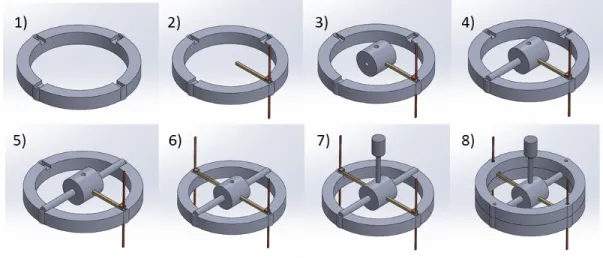
2.10 Assembly procedure of AVS with CAD drawings . . . 17

2.11 Adhesion of PZT beam and copper plates . . . 18

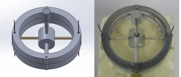
2.12 CAD drawing and actual assembly of AVS . . . 18

3.1 The cantilever beam under a point load at the free end [8] . . . . 21

3.2 Schematic of radius of curvature . . . 22

3.3 The first six mode shapes of AVS . . . 26

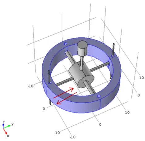
3.4 Harmonic load applied to bases of AVS. The arrows indicate the direction of movement of the sensor under the harmonic load. . . 27

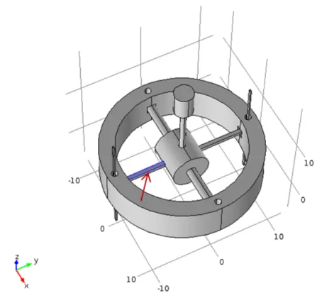
3.5 The data point chosen to detect the change in displacement . . . 28

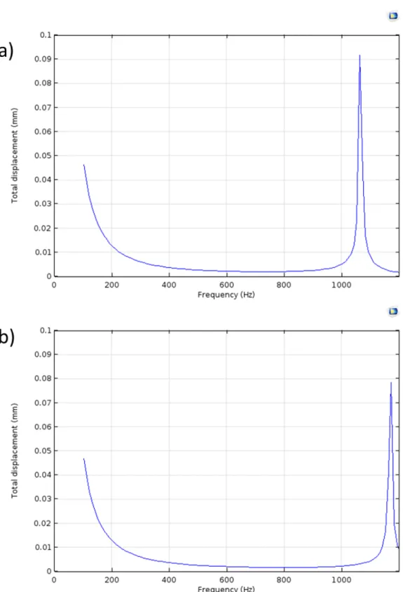
3.6 The change of displacement at the point chosen a) in y-direction b) in x-direction along the frequency range . . . 29

3.7 The top surface of PZT arm chosen to detect the voltage output . 30 3.8 The voltage output of the sensor in a) y-axis b) x-axis along the frequency range . . . 31

3.9 The directivity pattern of the sensor in y-axis at 1000 Hz . . . 32

3.10 The directivity pattern of the sensor in x-axis at 1000 Hz . . . 32

3.11 The manufacture model of AVS where the gaps are filled with adhesive material showing with blue . . . 33

LIST OF FIGURES xi

3.12 The first six mode shapes of manufacture model of AVS . . . 34

3.13 The change of displacement at the point chosen a) in y-direction b) in x-direction along the frequency range in manufacture model 36 3.14 The voltage output of the sensor in a) y-axis b) x-axis along the frequency range in manufacture model . . . 37

3.15 The directivity pattern of the sensor in y-axis at 1000 Hz in as-sembly effects model . . . 38

3.16 The directivity pattern of the sensor in x-axis at 1000 Hz in as-sembly effects model . . . 38

4.1 The vibration controller used in the test setup . . . 40

4.2 The power amplifier used in the test setup . . . 41

4.3 The controller and power amplifier . . . 41

4.4 The electro-dynamic shaker used in the test setup . . . 42

4.5 The miniature accelerometer used in the test setup . . . 43

4.6 The software of the vibration controller used in the test setup . . 44

4.7 The oscilloscope used in the test setup . . . 44

4.8 The shaker apparatus designed to mount three-axial base . . . 45

4.9 The three-axial base designed to mount sensors on top of it . . . . 46

4.10 Experimental setup . . . 47

LIST OF FIGURES xii

4.12 Frequency response of Sensor 1 in a) x axis b) y axis . . . 50

4.13 Comparison of frequency responses of Sensor 1, FEA Model and FEA Model with Assembly Effects . . . 51

4.14 Frequency response of Sensor 2 in a) x axis b) y axis . . . 52

4.15 Comparison of frequency responses of Sensor 2, FEA Model and FEA Model with Assembly Effects . . . 53

4.16 Directivity pattern of Sensor 1 at 1000 Hz . . . 53

4.17 Directivity pattern of Sensor 2 at 1000 Hz . . . 54

4.18 Experimental Setup of One Sensor . . . 55

4.19 Directivity pattern of Channel 1 at 1000 Hz . . . 56

4.20 Directivity pattern of Channel 2 at 1000 Hz . . . 56

5.1 Future three-dimensional design of AVS . . . 58

5.2 Planned packaging of AVS . . . 58

A.1 MB Dynamics Model 25 Shaker . . . 65 A.2 Dytran Instruments Model 3035BG Miniature IEPE Accelerometer 66

List of Tables

3.1 First six natural frequencies of µ-AVS . . . 25 3.2 Comparison of first six natural frequencies between rigid model

and manufacture model . . . 33

A.1 Basic specifications of the electro-dynamic shaker . . . 64 A.2 Basic specifications of the miniature accelerometer . . . 65

Chapter 1

Introduction

1.1

Introduction

Despite people have mostly started their studies on sound detection and commu-nication underwater in the twentieth century, some animals such as dolphins and bats are known to make use of sound to navigate and communicate. The first recorded contribution to underwater acoustics came from Leonardo Da Vinci in 1490 by discovering that sound travels in waves. After the dramatic sink of Ti-tanic, great interest on underwater acoustics has been observed and many patents have started to appear on this topic [1]. During World War I, underwater sens-ing systems have been developed to detect the enemies vessels such as British ‘ASDIC’ and American ‘SONAR’ (Sound Navigation And Ranging)[9]. A French scientist, Paul Langevin, has built an echo-ranging system in 1917 for the first time by using the piezoelectric effect which was discovered by Paul-Jacques and Pierre Curie in 1880[10]. During World War II and Cold War, both theoretical and experimental studies have been focused on this topic and this lead to a strong background of humans about underwater acoustics.

Hydrophones are used to listen to underwater sound. They are similar to mi-crophones since mimi-crophones measure sound in air whereas hydrophones do it

Figure 1.1: An example of SONAR system [1]

in water. The first hydrophone was Fessenden oscillator which was designed as underwater telegraph at first in 1914[11]. Most hydrophones are omnidirectional that means acoustic sounds from every directions are collected with the same sen-sitivities. In order to determine the direction of the incoming wave, hydrophones in form of an array are positioned with intervals and the time delays of sound among hydrophones gives the direction information where this phenomenon is called direction of arrival (DOA). However, it is much simpler to determine the direction with Acoustic Vector Sensor (AVS).

An Acoustic Vector Sensor is a device used to detect underwater acoustic signals by converting mechanical energy of the incident wave to a detectable electrical energy [12][13]. It is different from conventional hydrophones since it can measure the direction of the incident wave as well as the pressure differences whereas omnidirectional hydrophones only measure the pressure differences on their own. Most vector sensors make use of piezoelectric materials which generate an electric charge when a mechanical stress is applied.

Nowadays, vector sensors have found widespread acceptance because of their advantages over conventional hydrophones including the capability of sensing di-rection in addition to scalar pressure, feasibility of getting smaller dimensions,

Figure 1.2: The Fessenden oscillator[2]

Figure 1.3: An early hydrophone[3]

stronger signal to noise ratio (SNR) with just focusing on the direction of the sig-nal interested and getting out of the directions of noise, having higher sensitivity at low frequencies and lower cost [4, 5, 14, 15].

When these multiple advantages of acoustic vector sensors are taken into con-sideration, there have been lots of studies regarding this issue. In order to sense the direction of the acoustic sound, vector sensors detect either acceleration, velocity or pressure gradient. MEMS based piezoresistive vector sensors are de-signed with an inspiration from the auditory principle of fish. The lateral line of a fish provides to detect the movements in water and this line organ takes place from the head to the tail all the way through. It involves lots of stitches and each

Figure 1.4: Examples of commercial hydrophones

stitch involves lots of neuromasts. Each neuromast involves lots of hair cells where their top is receptor structure stereocilia. When this structure is excited with any signal like turbulence, there occurs changes in synapses connected to the nerve fiber. By inspiring this detection principle of fishes, MEMS based piezoresistive vector sensors are designed. The piezoresistors are placed onto the four beam structure forming a Wheatstone bridge circuit. When the sensing tip is excited with an acoustic signal, the stress on the beams causes changes in resistances of the piezo elements [4, 5, 16, 17, 18, 19]. An alternative sensor is fiber optic vector sensor in which fiber is deformed with the inertial force of the acoustic signal. The wavelength of the fiber changes in this situation and the acceleration information can be obtained by the shift in wavelength of the fiber[6, 20, 21, 22]. There are also capacitively sensed vector sensors which are pressure gradient just like piezoelectric ones. The flexible electrode in a parallel plate capacitor deflects with the pressure of incident wave and this leads to capacitance change which

provides the detection of that incident wave[7, 23, 24]. Also, acceleration and ve-locity vector sensors have taken places used for sensing the direction of acoustic sounds underwater[25, 26, 3, 27].

Figure 1.5: Fish audition principle [4]

These vector sensors have made some achievements on spatial gain, miniatur-ization and low frequency sensitivity, however, the fabrication of those sensors are all based on nano/micro manufacturing techniques including lithography, etching and deposition. This leads to both spending too much efforts and higher costs. Especially for prototype fabrication purposes, the aforementioned processes are not economically feasible. The use of mechanical micromachining can eliminate the need for expensive clean room facilities.

1.2

Motivation and Contribution

In this thesis, a novel acoustic vector sensor (AVS) has been designed based on two parallel piezoelectric cantilever beams attached to a mechanical sensing tip. The

Figure 1.6: Examples of vector sensors: a-b) Piezoresistive [4][5] c-d) Fiber optic [6] e-f) Capacitively sensed [7]

designed sensor uses piezoelectric elements (PZTs) to convert mechanical strain into sensible electrical signal. The design of the overall sensor is modular since each individual sensing element could be easily changed, tested and assembled. All parts of the sensor has been fabricated by mechanical micromachining and assembled together in a precise way, which increases design and manufacturing flexibility. This fabrication method also makes it preferrable due to providing lower cost and less effort.

The requirements of the designed sensor are determined consulting with our sponsor company (Meteksan Defense Inc.) as working in the frequency range 0-1 kHz, 8-shape directivity pattern when rotated with 15 degree and showing detectable voltage difference between 0 and 90 degree excitations.

The rest of the thesis is divided into sections as the following:

In Chapter 2, the mechanical design and manufacturing of AVS is presented. The dimensions of each parts used to form the sensor are introduced in a detailed way with the importance of each ones. Also, the working principle of µ-AVS is detailed in this chapter. Lastly, the fabrication processes of each parts of AVS and the assembly of the parts to form the sensor precisely are discussed.

Chapter 3 focuses on the modeling of the AVS. The mathematical formulation and finite element analysis are investigated. The finite element analysis is impor-tant to direct us before fabrication and for the characterization the sensor. First, modal analysis is done and natural frequencies and vibration modes are obtained. The harmonic response of the sensor is also investigated under forced vibration.

Chapter 4 explains the experimental setup, the vibration experiments per-formed and the results. The experiments are perper-formed with a well-controlled vibration platform in air to investigate the performance of sensing direction of AVS. In additon, the comparison of results between finite element analysis and experiments are presented.

Chapter 5 is the last chapter and conclude this thesis. Conclusions and possible future applications and improvements for the sensor are discussed.

Chapter 2

Design and Manufacturing

In this chapter, the design and manufacturing of AVS are presented. Firstly, the acoustics theory of a small cylinder immersed in fluid is presented. Secondly, the parts that are designed to form the sensor as an assembly are detailed with their dimensions and importance. Thirdly, the working principle of µ-AVS, based on piezoelectric effect and directions of PZT arms, is reported. Lastly, it is explained how the parts are manufactured and assembled together.

2.1

Theory

According to the acoustic theory, if a small cylinder given in Fig 2.1 is immersed in fluid and the wavelength of the incident plane wave is much bigger is the radius of the cylinder, the acoustic force exerting on the cylinder in x axis is [3, 5]

Fx = −2jp0kHπa2 (2.1)

where p0 is the acoustic pressure applied on the cylinder, k is the wave number of

the sound wave, a is the radius of the cylinder and H is the height of the cylinder. When this relation and the relation for radiant impedance of pendular cylinder

Figure 2.1: The incoming plane wave and small cylinder immersed in fluid are calculated together and ka << 1, the velocity of the cylinder in x direction is known as

Vx=

2ρ0

ρ0+ ρ

V0 (2.2)

where ρ0 is the density of the fluid, ρ is the density of the cylinder and V0 is the

velocity magnitude of the fluid. It means that if the densities of the cylinder and the fluid are equal, the velocity of the cylinder will be equal to the velocity of the fluid. In other words, the motion of the cylinder whose density is equal to the density of the fluid will be the same with the motion of the fluid particles at low frequencies [5].

2.2

Parts used in the Design

For the design of the sensor, the designs in literature [4, 5, 16, 17] are taken as guides to check feasibility and our capability in terms of fabrication. For the initial designs, cables were soldered to the top and bottom surfaces of PZT beams to read the data, but this option led to cracks on the beams frequently when cables are moved. Therefore, copper plates touching the top and bottom surfaces of

Figure 2.2: Early try of the sensor

PZT beams are added to the design. Then in the next version of the sensor, we observed that the whole body of the sensor vibrates instead of vibration of the sensing tip in the direction of the movement. To eliminate this effect, cylindrical metal rods and connection mass are preferred to help the sensing tip to roll onto the PZT arms more in direction of movement. Also, a mass is added to the top of the sensing tip to increase the beam deformation and therefore voltage on PZTs when stimulated.

The basis of the design of the sensor presented here is to capture the motion of the acoustical particle at the tip of the sensor when an input is provided. Figure 2.3 illustrates the solid model of the designed sensor, as it can be seen from this figure, the sensor is composed of six major parts.

Figure 2.3: The solid model of AVS design

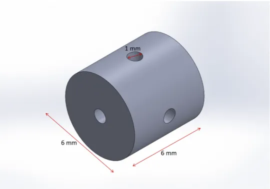
Figure 2.5: The schematic of the connection mass

2.2.1

Mechanical Sensing Tip

It is in form of a cylindrical rod with a mass on top of it. The tip diameter is 1 mm and the top is 3 mm. The length of the rod is 9 mm and the top is 4 mm. There exists a conical part between the rod and the mass at the top and it is 1 mm long. So, its total length is 14 mm. It applies a torque onto the PZT beams when it is stimulated with an acoustic signal.

2.2.2

Connection Mass

It has been designed in the form of a cylinder with a dimension of 3 mm radius and 6 mm long. It is drilled thrice with a radius of 0.5 mm with 90 degrees. This part acts as a support for PZTs and mechanical sensing tip. Six notches have been designed for positioning and fixing PZTs.

Figure 2.6: The schematic of the PZT beam

2.2.3

PZT Beams

Two PZT beams have been designed fixed to the base at one end and to the connection mass at the other end. The length of these beams is 10 mm, width and thickness is 0.6 mm. These PZTs are commercially available and they have been purchased from the company Morgan Technical Ceramics. They generate voltage when it is deformed by the mechanical sensing tip.

2.2.4

Copper Plates

They are designed to be mounted at the ends of PZTs to provide easy soldering. Instead of soldering on top and bottom surfaces of PZT beams directly to measure the electrical signals, it is easier and more secure to touch these plates while measurements. The plates are 9 mm long, 0.4 mm width and 0.2 mm thick. Also, a square block has been designed at one end of these plates with dimensions

Figure 2.7: The schematic of the copper plate

1x1x0.2 mm. These blocks make contacts with top and bottom surfaces of the PZT beams for measuring voltage values.

2.2.5

Bases

It has a circular shape with a hole inside and keeps the whole parts together. The two bases have been attached to fix the PZT beams and metal rods at one end and the notches on these bases take places to mount metal rods, PZT beams and copper plates. The radii of the base and its hole are 12.5 and 10 mm respectively and its thickness is 3 mm.

2.2.6

Metal Rods

Two metal rods designed to roll the mechanical sensing tip with the connection mass onto the PZT beams easily to sustain more deformation.They are fixed at

Figure 2.8: The schematic of the base

one end to the bases and shrinked to the connection mass at the other end. The bigger diameter is 1.5 mm with 9 mm long and smaller diameter is 1 mm with 2.5 mm long.

2.3

Working Principle of the Design

The working principle of AVS is based on the piezoelectric effect and the direction of stands of PZT beams: When the sensing tip is excited with the motion of the sensor due to an acoustic signal, strain on the PZT beams generates voltage by piezoelectric effect. This voltage is transferred to electronic circuit using the copper plates that are mounted at the ends of these beams. The torque applied onto the beams by the sensing tip when stimulated is higher when the PZT beams stand in the same direction with the acoustic signal. Therefore, it is possible to understand which direction the acoustic wave propagates by reading the voltage differences from PZT beams. The metal rods help the connection mass and the

Figure 2.9: The schematic of the metal rod

sensing tip attached on top to roll onto the PZT beams, therefore higher voltage differences can be obtained in this way.

2.4

Manufacturing and Assembly Procedure

All parts of the sensor have been fabricated using mechanical micromachining processes and assembled together except for PZT beams. The mechanical sensing tip and metal rods have been fabricated by µ-turning process on a 3 mm Al 6061 alloy. Bases and connection mass have been fabricated on a Poly (methyl methacrylate) (PMMA) part using micro milling and turning processes. In order to fabricate copper plates, a laser micromachining center has been used. A pulsed fiber laser with a wavelength of 1064 nm, output power of 10 W, pulse width of 80-120 nm and a spot size of 30 µm is used. The PZT beams and copper plates are glued with silver filled epoxy and ovened at 120 C degree for 2 hours. This is preferred for reading voltages on PZT beams easily instead of soldering cables to the top and bottom surfaces of PZTs. The copper plates are then twisted with

Figure 2.10: Assembly procedure of AVS with CAD drawings 90 degree for assembling.

After fabrication of all parts are completed, they are assembled together as depicted in Fig 2.10. All the touching parts are glued with metal epoxy among each other except for the connection between metal rods and connection mass. The reason is to roll the connection mass and sensing tip more with the help of metal rods and to create higher torque on PZT beams, therefore, higher voltage on them.

Figure 2.11: Adhesion of PZT beam and copper plates

Chapter 3

Modeling

In this chapter, mathematical and computational modeling of AVS is presented. Firstly, the mathematical formulation based on the Euler Bernoulli beam the-ory is investigated to predict the behaviour of the mechanical sensing tip under loading and the natural frequencies of the sensor. Secondly, the finite element analyses of µ-AVS have been done in finite element analysis software (COMSOL Multiphysics) to check the dynamic properties of the design and to give us a direction about fabrication. The natural frequencies and vibration modes of the sensor have been investigated which has an importance to determine the work-ing bandwidth of the sensor. Then, the body of the sensor is vibrated with a sinusoidal signal along the frequency domain and the response of the sensor to this signal is investigated. Also, the directivity pattern of µ-AVS is obtained with applying a rotating load. Lastly, a model closer to manufactured sensor is examined by adding the glue effect to the previous model and these two models are compared at the end.

3.1

Mathematical Formulation

To investigate the possible responses of µ-AVS design under both free and forced vibrations, the beam theory is used in this section. The maximum deflection of a rod which corresponds to the sensing tip in our design is formulated and the natural frequencies of that rod, which are important to determine the working bandwidth, are also derived.

3.1.1

Maximum Deflection of a Rod Fixed at One End

The maximum deflection of a rod fixed at one end is going to be formulated when a point load is applied at the free end. The bending equation is known as [28]:

M I = E R → 1 R = M EI (3.1)

where M is the bending moment, I is the moment of inertia, E is the elastic modulus and R is the radius of curvature of the beam surface to the bending moment. Mathematically, the radius of curvature can be expresses as

1 R = d2x dy2 [1 + (dx dy) 2_]3₂ (3.2)

where the slope term dx_dy is very small, so the equation can be simplified as 1

R ≈ d2_x

dy2 (3.3)

So, the equation becomes

d2x dy2 = −

F y

EI (3.4)

where M = −F y is this situation. Rearranging yields EId

2_x

dy2 = −F y (3.5)

Integration with respect to y gives

EIdx = −F y

2

Figure 3.1: The cantilever beam under a point load at the free end [8] The boundary condition gives that for y = L, dx/dy = 0. So,

0 = −F L

2

2 + A → A = F L2

2 (3.7)

Therefore, the equation becomes EIdx

dy = − F

2(y

2_{− L}2_{) (3.8)}

Integrating again gives

EIx = −F y

3

6 + F L2_y

2 + B (3.9)

The boundary condition is y=L, x=0. So, 0 = −F L 3 6 + F L3 2 + B → B = − F L3 3 (3.10) Hence, the relation becomes

EIx = −F y 3 6 + F L2_y 2 − F L3 3 (3.11)

The aim is to find the deflection at the free end y = 0. EIxD = −

F L3

3 → xD = − F L3

Figure 3.2: Schematic of radius of curvature

3.1.2

Natural Frequency of a Rod Fixed at One End

To calculate the natural frequencies of a rod fixed at one end, the Euler-Bernoulli beam equation is used [29]:

EI∂

4_y

∂4_x = −ρA

∂2_y

∂2_t (3.13)

By using separation of variables, we can get

y(x, t) = X(x)T (t) (3.14) So, the equation becomes

−EI ρA 1 X(x) d4X d4_x = 1 T (t) d2T d2_t (3.15)

If b is a constant, one can get −EI ρA 1 X(x) d4X d4_x = 1 T (t) d2T d2_t = −b 2 _(3.16)

Rearranging results d2_T d2_t + b 2_{T (t) = 0 (3.17)} d4_X d4_x − b 2 (ρA EI)X(x) = 0 (3.18) The solution of this fourth-order equation is [30]

X(x) = C1sin(λx) + C2cos(λx) + C3sinh(λx) + C4cosh(λx) (3.19)

where

λ = (b2(ρA EI))

1

4 (3.20)

The boundary conditions in this problem are:

X(0) = 0 (3.21) dX dx|x=0 = 0 (3.22) d2_X dx2 |x=L= 0 (3.23) d3_X dx3 |x=L= 0 (3.24)

When these boundary conditions are used, the solution is

cos(λL)cosh(λL) = −1 (3.25) There is not unique root for λ, so the subscript n should be added

cos(λnL)cosh(λnL) = −1 (3.26)

By using the Newton-Raphson method, an approximate numerical solution can be found as [31]

λnL ≈

(2n − 1)π

2 (3.27)

So, the time-dependent equation becomes T (t) = d1sin[(λ2n s EI ρA)t] + d2cos[(λ 2 n s EI ρA)t] (3.28)

The frequency from this equation is ωn = λ2_n L2 s EI ρA (3.29)

where its unit is rad/s. If we convert it to Hz, the natural frequency formula is fn = λ2_n 2πL2 s EI ρA (3.30)

The first three natural frequencies are calculated as [30] f1 = (1.8751)2 2πL2 s EI ρA (3.31) f2 = (4.6941)2 2πL2 s EI ρA (3.32) f3 = (7.8539)2 2πL2 s EI ρA (3.33)

For an aluminum rod with 9 mm long like in our design, the first three natural frequencies are found as 8789, 52913 and 140026 Hz respectively. However, there exists a mass part with 3 mm radius and 5 mm long in our design to create more deformation on the PZT beams. This geometrical difference affects the results considerably, so it is better to use finite element analysis for such complex geometries.

3.2

Finite Element Analysis

Mathematical formulation is useful for a single part and for simple geometries. However, the mechanical sensing tip in our design has a much complex geometry difficult to formulate and different materials take places in the design. Therefore, using finite element analysis is more meaningful for our design while characterizing the sensor.

Table 3.1: First six natural frequencies of µ-AVS Mode Number 1 2 3 4 5 6 Nat. Freq. (Hz) 1071 1159 4287 8498 9314 12601

3.2.1

Vibration Modes and Natural Frequencies of AVS

The natural frequency is the frequency that the object oscillates without any external force. If there exists a forced vibration at a frequency that is the same with the natural frequency of that object, it will create much larger amplitude at that frequency and this phenomenon is called resonance. The mode shape is the harmonic motion of the object at the natural frequency.

The working bandwidth of the AVS is from 0 Hz to the first natural frequency. It means that the frequency range is safe to be worked out in the absence of any resonance. As it is shown in Fig 3.3 and Table 3.1, the first vibration mode is in y direction and have a natural frequency of 1071 Hz. The second mode is in x-direction and its natural frequency is close to the first one with 1159 Hz. It is usually not preferred to have x, y natural frequencies close to each other, but it is needed to change the geometry to make them further. The third frequency is in z-direction with a natural frequency of 4287 Hz. The fourth, fifth and sixth frequencies are very far from the working bandwidth. As a result, the working bandwidth of the sensor is from 0 to 1071 Hz according to this simulation.

3.2.2

Frequency Response of AVS

In order to examine the response of AVS under any load, a harmonic boundary load is applied through a frequency range. Frequency response of the sensor has been analyzed with a simulation that the bases of the sensor are vibrated with a 2 g acceleration in y-axis along the frequency domain of 200-1200 Hz (Fig.3.4). Fig. 3.6a shows the change in displacement of a point on top of the sensing tip in y-axis (Fig 3.5) and the resonance frequency has a well overlap with modal analysis. The frequency range from 0 to 1071 Hz is eventually found safe without

Figure 3.4: Harmonic load applied to bases of AVS. The arrows indicate the direction of movement of the sensor under the harmonic load.

any resonance. The change of displacement in x-axis is shown in Fig 3.6b where the peak is at 1159 Hz which is the natural frequency of the second vibration mode occurs in x-axis.

The outputs in the graphs decrease at low frequencies while frequencies are increasing. The reason is that the acceleration a is constant with the magnitude 2 g, frequency w increases, so displacement x decreases according to the relation a = w2_{x. This leads to decrease in deformation at PZT arms. But, after a certain}

frequency, the sensor feels the effect of resonance and the output increases with the frequency.

Also, the voltage that arises by the piezoelectric effect on the PZT arms is examined with the same boundary load in y-axis. Fig.3.8a shows the voltage output of the sensor as a function of the frequency. It is clear that the resonance occurs at the first natural frequency 1071 Hz.

Figure 3.5: The data point chosen to detect the change in displacement The same simulation is done again but the load is applied to the bases in x-axis this time. The PZT arms are located in y-direction, so it is expected the voltage output in this simulation should be much less than the one in y-axis. It is seen in Fig 3.8b that the voltage differences along the frequency range in x and y axes are really high which is important to determine the direction of an incoming wave.

3.2.3

Directivity Pattern of AVS

Directivity pattern exhibits the ability of the sensor to determine the direction of any signal. To obtain this pattern, a rotating load with 5 degrees is applied to the mechanical sensing tip with the magnitude 1cos(θ) N at 1000 Hz. Fig.3.9 shows that the sensor has an 8-shape directivity pattern which indicates when a signal comes from the parallel direction of PZT arms, the deformation on those arms is the highest, therefore the voltage output is maximum there. However, when a signal comes perpendicular to the PZTs, the mechanical sensing tip will also vibrate perpendicular to them, then the voltage output will be the minimum.

Figure 3.6: The change of displacement at the point chosen a) in y-direction b) in x-direction along the frequency range

Figure 3.7: The top surface of PZT arm chosen to detect the voltage output

3.2.4

Model of AVS with Assembly Effects

The model is created above with great precision according to the design, however, the assembly created after manufacturing of the parts may exhibit notable dif-ferences in reality. The parts are glued to each other while creating assembly of AVS and this remarkably effects the characteristics of the sensor. To investigate this effect in depth, a more realistic model is created and the same simulations above are repeated to compare the results. As shown in Fig. 3.11, the gaps are filled with adhesive material in the model just as filling in assembly process.

The mode shapes in this model are in the same directions with the former model, but the natural frequencies change significantly as shown in Table 4.2. The first natural frequency is found as 964 Hz in this analysis which turns the working bandwidth 0 to 964 Hz.

Figure 3.8: The voltage output of the sensor in a) y-axis b) x-axis along the frequency range

Figure 3.9: The directivity pattern of the sensor in y-axis at 1000 Hz

Figure 3.11: The manufacture model of AVS where the gaps are filled with ad-hesive material showing with blue

Table 3.2: Comparison of first six natural frequencies between rigid model and manufacture model

Mode 1 2 3 4 5 6

Nat. Freq. of Rigid Model (Hz) 1071 1159 4287 8498 9314 12601 Nat. Freq. of Manuf. Model (Hz) 964 1055 4027 8061 8349 13534

model. The voltage and displacement data preserve the same trend, but the magnitudes reduce slightly. The reason is the damping caused by adhesion among the parts used in assembly.

The directivity patterns again remain the same 8-shapes, but there are slight reductions in magnitudes due to the damping effect.

Figure 3.13: The change of displacement at the point chosen a) in y-direction b) in x-direction along the frequency range in manufacture model

Figure 3.14: The voltage output of the sensor in a) y-axis b) x-axis along the frequency range in manufacture model

Figure 3.15: The directivity pattern of the sensor in y-axis at 1000 Hz in assembly effects model

Figure 3.16: The directivity pattern of the sensor in x-axis at 1000 Hz in assembly effects model

Chapter 4

Experimental Setup and

Experiments

In Chapter 3, the dynamic and harmonic properties of AVS are investigated with two models created in finite element analysis. The natural frequencies, frequency responses and directivity patterns of the sensor are examined for the characterization. In this chapter, the characterization of manufactured sensor is made with some tests using a well-controlled vibration platform. Since the tests in any sound absorbing pool require well-packaging and difficulty of manipulation, the very first tests of the prototype have been conducted on a vibration platform in air.

Firstly, the equipments used in the test setup will be presented in this chapter. Then, the experimental setup and the procedure of performing the tests will be examined. Lastly, the results of the tests will be conveyed and a comparison of finite element analysis and experimental results will be discussed.

Figure 4.1: The vibration controller used in the test setup

4.1

Equipment Used in the Test Setup

There are six main equipments used in the setup for performing a controlled vibration test of AVS.

4.1.1

Vibration Controller

It is a PC-based closed-loop controller with 8 input channels. The publisher company of this device is Data Physics. It has an embedded PC inside and it can be controlled via a host PC.

4.1.2

Power Amplifier

It provides to increase the power of any signal, that means, it provides gain to the system. Its model is MB Dynamics MB500VI. It has both AC and DC input coupling selectable. Its feedback mode can be switched as voltage or current with an external button. Its maximum frequency usable is 20 kHz.

Figure 4.2: The power amplifier used in the test setup

Figure 4.4: The electro-dynamic shaker used in the test setup

4.1.3

Electro-Dynamic Shaker

It is a device to excite any workpiece connected to it with a sinusoidal, random or shock signal given by controller and software. Its model is MB Dynamics Modal 25. 110 N peak force and 25 mm peak-to-peak stroke can be obtained via this device. The maximum frequency that can be applied on it is 4 kHz.

4.1.4

Accelerometer

It is a device used to measure acceleration during vibration and give feedback to the controller to fix the acceleration to the desired value. Its publisher company is Dytran Instruments. It has a reference sensitivity value of 9.61 mV/g and its working bandwidth is from 0.5 to 10000 Hz. It is mounted perpendicular to the motion with an adhesive material. Its sensing material is piezoceramic and the outer part is made of stainless steel.

Figure 4.5: The miniature accelerometer used in the test setup

4.1.5

Software

The software of the vibration controller is SignalStar Scalar. It enables to adjust the parameters such as frequency, acceleration and time duration of the test. Also, the working mode like random, sine, shock can be selected using this software.

4.1.6

Oscilloscope

It is used to display data coming from the test environment. Its model is GW INSTEK GDS1052U. It has two input channels. It is possible to make some operations such as adding, substracting and FFT with using the data coming from two input channels. Also, there is a USB port to gather the data directly.

4.2

Experimental Setup

An experimental setup is built to conduct the experiments of AVS by using the equipments mentioned above.

Figure 4.6: The software of the vibration controller used in the test setup

Figure 4.8: The shaker apparatus designed to mount three-axial base As a host PC, the user PC is connected to the PC embedded in the vibration controller. A sinusoidal signal with the magnitude of 2 g acceleration is adjusted via the software of the controller. The controller is connected to the software, power amplifier and the accelerometer. The power amplifier is adjusted to AC mode and the gain is adjusted manually enough to reach the desired magnitude of the signal. The electro-dynamic shaker is positioned horizontally and connected to the power amplifier to transmit the amplified signal.

An apparatus (Fig 4.8) is designed to mount the sensors to the shaker and it is mounted to the moving part of the shaker. There is a big hole at the center of the apparatus to pass the cables down and four holes near the corners for screwing and fixing the sensors. Also, four connection parts take places perpendicularly for rotating the sensors easily while mounting to the shaker.

A three-axial base is also prepared to mount three AVSs to the vibration platform at the same time. As it is seen in Fig 4.9, there exist three altitudes

Figure 4.9: The three-axial base designed to mount sensors on top of it that three sensors are going to be positioned and holes for passing the solder wires and for screwing.

The three-axial base is fixed on top the shaker apparatus with screwing and two sensors are fixed on top of the three-axial base with again screwing. The third axis is left blank for simplicity now. Wires are soldered to the ends of the copper plates to read the voltage differences on the PZT arms. Then, the other ends of the wires are clipped with electronic cables and those cables are connected to the input channels of the oscilloscope to gather the voltage outputs.

4.3

Results of the Experiments

The experiments are performed with two sensors, Sensor 1 is in x axis, Sensor 2 is in y axis shown in Fig 4.10 and 4.11 on a three axial base. The frequency response of the sensors is investigated in a frequency range 600-1200 Hz. As Fig 4.12 and

Fig 4.14 show, the first natural frequencies are found at 965 and 1140 Hz. The difference arises from the manufacturing and assembly process. According to the original design, the mechanical sensing tip should be stuck in through the hole on the connection mass with 1 mm long like Sensor 1. However, for Sensor 2, that dimension is 2 mm that’s why the natural frequency is found higher than the frequency of Sensor 1.

Fig 4.13 presents the comparison among the results of FEA model, FEA model with assembly effects and experimental results of Sensor 1. It can be seen that resonant peaks of model with assembly effects and experiments appears at the nearly same frequency. The magnitude of the experimental result at resonance is found lower, the reason could be that the exact resonant frequency point may not be hit during the experiments.

As it is seen in Fig 4.15, the experimental result of Sensor 2 has a well overlap with the FEA model with assembly effect which is modified to the assembly geometry of Sensor 2.

The directivity patterns are also obtained by rotating and taking data from two sensors with 15 degree steps at 1000 Hz. As shown in Fig 4.15 and 4.16, they are not exactly in the shape of 8 like in FEA results. The reason could be that the three axial base is not symmetric along the direction of movement. In other words, the center of mass of that part is not at the center of it.

The experiments are repeated with one sensor to eliminate the symmetry prob-lem since it is symmetric in both x and y directions. The data taken from both channels at 1000 Hz and directivity patterns are obtained with them. As they are seen in Fig. 4.19 and 4.20, they have similar 8-shape directivity patterns with FEA models. It is not possble to get 0 mV data in experiments due to noise whereas it is sure to get it in FEA with sin(θ) and cos(θ) terms at 0 and 90 degrees respectively.

Figure 4.13: Comparison of frequency responses of Sensor 1, FEA Model and FEA Model with Assembly Effects

Figure 4.15: Comparison of frequency responses of Sensor 2, FEA Model and FEA Model with Assembly Effects

Figure 4.19: Directivity pattern of Channel 1 at 1000 Hz

Chapter 5

Conclusion and Future Work

The design of a novel Acoustic Vector Sensor is presented in this thesis. Individual parts which are manufactured via mechanical micromachining come together to form this sensor. Two parallel piezoelectric elements take places in this design which generate voltage differences when stimulated with the help of sensing tip and metal rolling rods.

The modeling of AVS is investigated by mathematical formulation and finite element analysis. The vibration modes and natural frequencies of the sensor are obtained and the working bandwidth is determined as 0 to 1 kHz approximately. The frequency response and directivity pattern of the sensor are investigated using finite element analysis. Also, a model including the assembly effects is created to see the damping effect of the adhesion while assemblying.

The experiments are performed in a well controlled vibration platform. The setup mainly includes the equipments controller, amplifier, shaker and software. Two sensors are used in x and y axes during the experiments. The frequency re-sponse and directivity patterns, which have the same trend with the ones found in finite element analyses with an acceptable deviation, are obtained.Vibration tests are used in this thesis to characterize the sensor for both FEA and experimental studies based on acoustic particle motion principle explained in Chapter 2.1, so

Figure 5.1: Future three-dimensional design of AVS

Figure 5.2: Planned packaging of AVS some acoustic tests are planned to be performed in future.

Adding the third dimension sensor is planned for the near future. As it is shown in Fig 5.1, the rectangular bases are planned to be used for the z-direction. The sensor is going to be mounted vertically for determining the direction in z axis.

Packaging and testing in a standing wave tube is another future plan. Fig. 5.2 shows the pending work which may differ the characteristics of the sensor underwater.

This vector sensor is designed for the detection of acoustic signals underwater, however, it is possible to use the sensor for different purposes with some slight changes. It could be used in air as a micro-coordinate measuring machine (CMM)

by adding a probe on top of it [32]. Also, using as a resonant sensor is another option for this sensor. For example, it is possible to detect the acceleration by checking the changes in resonance frequency of the sensor in air [33].

Bibliography

[1] V. A. Kaharl, Sounding Out the Ocean’s Secrets. National Academey of Sciences, 1999.

[2] G. L. Frost, “Inventing schemes and strategies: The making and selling of the fessenden oscillator,” Technology and Culture, vol. 42, no. 3, pp. 462–488, 2001.

[3] C. Leslie, J. Kendall, and J. Jones, “Hydrophone for measuring particle velocity,” The Journal of the Acoustical Society of America, vol. 28, no. 4, pp. 711–715, 1956.

[4] C. Xue, S. Chen, W. Zhang, B. Zhang, G. Zhang, and H. Qiao, “Design, fabrication, and preliminary characterization of a novel mems bionic vector hydrophone,” Microelectronics Journal, vol. 38, no. 10, pp. 1021–1026, 2007. [5] S. Chen, C. Xue, B. Zhang, B. Xie, and H. Qiao, “A novel mems based piezoresistive vector hydrophone for low frequency detection,” in Mecha-tronics and Automation, 2007. ICMA 2007. International Conference on, pp. 1839–1844, IEEE, 2007.

[6] J. Wang, H. Luo, Z. Meng, and Y. Hu, “Experimental research of an all-polarization-maintaining optical fiber vector hydrophone,” Journal of Light-wave Technology, vol. 30, no. 8, pp. 1178–1184, 2012.

[7] R. D. White, L. Cheng, and K. Grosh, “Capacitively sensed micromachined hydrophone with viscous fluid-structure coupling,” in MOEMS-MEMS Mi-cro & Nanofabrication, pp. 121–132, International Society for Optics and Photonics, 2005.

[8] C. Spoon and W. Grant, “Biomechanics of hair cell kinocilia: experimental measurement of kinocilium shaft stiffness and base rotational stiffness with euler–bernoulli and timoshenko beam analysis,” Journal of Experimental Bi-ology, vol. 214, no. 5, pp. 862–870, 2011.

[9] W. D. Hackmann, “Sonar research and naval warfare 1914-1954: A case study of a twentieth-century establishment science,” Historical Studies in the Physical and Biological Sciences, vol. 16, no. 1, pp. 83–110, 1986.

[10] A. Manbachi and R. S. Cobbold, “Development and application of piezoelec-tric materials for ultrasound generation and detection,” Ultrasound, vol. 19, no. 4, pp. 187–196, 2011.

[11] R. Blake, “Submarine signaling: The protection of shipping by a wall of sound and other uses of the submarine telegraph oscillator,” American In-stitute of Electrical Engineers, Proceedings of the, vol. 33, no. 10, pp. 1569– 1581, 1914.

[12] W. D. Zhang, L. G. Guan, G. J. Zhang, C. Y. Xue, K. R. Zhang, and J. P. Wang, “Research of doa estimation based on single mems vector hy-drophone,” Sensors, vol. 9, no. 9, pp. 6823–6834, 2009.

[13] P. Wang, G.-J. Zhang, C.-Y. Xue, W.-D. Zhang, and J.-J. Xiong, “Engi-neering application of mems vector hydrophone and self-adapting root-music algorithm,” in Solid-State Sensors, Actuators and Microsystems Conference (TRANSDUCERS), 2011 16th International, pp. 426–429, IEEE, 2011. [14] K. Madhavi, M. Krishna, and C. C. Murthy, “Design of a piezoresistive

micropressure sensor using finite element analysis,” International Journal of Computer Applications, vol. 70, no. 3, 2013.

[15] L. Guan, C. Xue, G. Zhang, W. Zhang, and P. Wang, “Advancements in technology and design of nems vector hydrophone,” Microsystem technolo-gies, vol. 17, no. 3, pp. 459–467, 2011.

[16] G.-j. Hang, Z. Li, S.-j. Wu, C.-y. Xue, S.-e. Yang, and W.-d. Zhang, “A bionic fish cilia median-low frequency three-dimensional piezoresistive mems vector hydrophone,” Nano-Micro Letters, vol. 6, no. 2, pp. 136–142, 2014.

[17] Z. Guojun, W. Panpan, G. Linggang, X. Jijun, and Z. Wendong, “Im-provement of the mems bionic vector hydrophone,” Microelectronics Journal, vol. 42, no. 5, pp. 815–819, 2011.

[18] X. Song, Z. Jian, G. Zhang, M. Liu, N. Guo, and W. Zhang, “New research on mems acoustic vector sensors used in pipeline ground markers,” Sensors, vol. 15, no. 1, pp. 274–284, 2014.

[19] G. Zhang, P. Zhao, and W. Zhang, “Resonant frequency of the silicon micro-structure of mems vector hydrophone in fluid-micro-structure interaction,” AIP Advances, vol. 5, no. 4, p. 041316, 2015.

[20] R. Ma, W. Zhang, and F. Li, “Two-axis slim fiber laser vector hydrophone,” Photonics Technology Letters, IEEE, vol. 23, no. 6, pp. 335–337, 2011. [21] J. Bucaro, H. Dardy, and E. Carome, “Fiber-optic hydrophone,” The Journal

of the Acoustical Society of America, vol. 62, no. 5, pp. 1302–1304, 1977. [22] D. J. Hill, P. J. Nash, D. A. Jackson, D. J. Webb, S. O’Neill, I. Bennion, and

L. Zhang, “Fiber laser hydrophone array,” in Photonics East’99, pp. 55–66, International Society for Optics and Photonics, 1999.

[23] R. I. Haque, C. Loussert, M. Sergent, P. Benaben, and X. Boddaert, “Op-timization of capacitive acoustic resonant sensor using numerical simulation and design of experiment,” Sensors, vol. 15, no. 4, pp. 8945–8967, 2015. [24] J. Li, L. Chen, Z. Gong, S. Xin, and M. Hong, “A low-noise mems

acous-tic vector sensor,” in Optoelectronics and Microelectronics (ICOM), 2013 International Conference on, pp. 121–124, IEEE, 2013.

[25] K. Kim, T. B. Gabrielson, and G. C. Lauchle, “Development of an accelerometer-based underwater acoustic intensity sensor,” The Journal of the Acoustical Society of America, vol. 116, no. 6, pp. 3384–3392, 2004. [26] H. K. Rockstad, T. W. Kenny, P. J. Kelly, and T. B. Gabrielson, “A

mi-crofabricated electron-tunneling accelerometer as a directional underwater acoustic sensor,” in Acoustic particle velocity sensors: Design, performance, and applications, vol. 368, pp. 57–68, AIP Publishing, 1996.

[27] J. L. Butler, S. C. Butler, D. P. Massa, and G. H. Cavanagh, “Metallic glass velocity sensor,” in Acoustic particle velocity sensors: Design, performance, and applications, vol. 368, pp. 101–133, AIP Publishing, 1996.

[28] L. Meirovitch, “Fundamentals of vibrations,” 2001.

[29] W. F. Stokey, “Vibration of systems having distributed mass and elasticity,” 1988.

[30] S. M. Han, H. Benaroya, and T. Wei, “Dynamics of transversely vibrat-ing beams usvibrat-ing four engineervibrat-ing theories,” Journal of sound and vibration, vol. 225, no. 5, pp. 935–988, 1999.

[31] T. Irvine, “Application of the newton-raphson method to vibration prob-lems,” Revision E, Vibrationdata, 2010.

[32] G. Dai, S. B¨utefisch, F. Pohlenz, and H.-U. Danzebrink, “A high precision micro/nano cmm using piezoresistive tactile probes,” Measurement Science and Technology, vol. 20, no. 8, p. 084001, 2009.

[33] C. Li, Y. Zhao, and R. Cheng, “A micro resonant acceleration sensor com-prising silicon support with temperature isolator and quartz doubled ended tuning fork,” in Nano/Micro Engineered and Molecular Systems (NEMS), 2014 9th IEEE International Conference on, pp. 346–349, IEEE, 2014.

Appendix A

Vibration Equipments

A.1

Electro-Dynamic Shaker

MB Dynamics Model 25 Shaker basic specifications are presented in Table (A.1). Its figure is given in Figure (A.1).

A.2

Miniature Accelerometer

Dytran Instruments Model 3035BG Miniature IEPE Accelerometer is used shown in Figure (A.2). Its spec summary is listed in Table (A.2).

Table A.1: Basic specifications of the electro-dynamic shaker Force 110 N peak forced air cooled; 55 N peak convection Stroke 25 mm p-p; 28 mm between stops

Bandwidth DC-4000 Hz Moving element 0.1 kg Shaker weight 14 kg

Dimensions 230 mm x 190 mm x 235 mm

Figure A.1: MB Dynamics Model 25 Shaker

Table A.2: Basic specifications of the miniature accelerometer Weight 2.5 grams

Sensitivity 10.2 mV/m /s2

Frequency Response 0.5 to 10000 Hz Maximum Vibration 600 Gpeak Maximum shock 10000 Gpeak Supply Current Range 2 to 20 mA Compliance Voltage Range 18 to 30 V Bias Voltage 11 to 13 V DC Discharge Time Constant 0.8 to 2 Sec