M.ŞENGÜL / IU-JEEE Vol. 11(2), (2011), 1407-1412
Synthesis of Resistively Terminated LC Ladder Networks
Metin ŞENGÜL
Kadir Has University, Dept. of Electronics Engineering, Engineering Faculty, 34083, Cibali-Fatih, Istanbul, Turkey
Tel: +90-212-533-6532, Fax: +90-212-533-4327 [email protected]
Abstract: In this work, element value calculation algorithms have been proposed for low-pass, high-pass,
band-pass and band-stop LC ladder networks. According to the calculated constant from the given transfer scattering matrix, the element type that will be extracted is decided. After calculating the element value, its transfer scattering matrix is obtained. Then transfer scattering matrix of the remaining network is calculated and the same procedure is applied until the termination resistance is reached. After explaining the algorithms, four examples are given to illustrate the utilization of the proposed method.
Keywords: Decomposition, LC Ladder Networks, Lossless Networks, Transfer Scattering Matrix.
1. Introduction
The filter synthesis, given a prescribed insertion-loss between a resistive source and a resistive load, is a classical procedure presented in many textbooks on network synthesis [1]-[3]. The method consists of, given the insertion-loss function, determining the squared-magnitude
2
) (
j of the reflection coefficient ( p), then getting a stable
( p), and, finally, deriving the corresponding driving-point impedance Z( p). From this Z( p), a lossless network terminated by a resistance can be found, satisfying the prescribed insertion-loss.If the problem under consideration is a broadband impedance matching problem, in this case, driving-point impedance Z( p) can be obtained via any existing method, i.e., line segment technique or simplified real frequency technique [4].
For some special data, the resulting Z( p)
can be developed in continued-fraction expansion, thus yielding a network in ladder form. Some work in the past obtained explicit formulas for the elements in ladder form for some configurations of the poles and zeros of ( p) [5]-[10]. For example, in [8], Orchard has given explicit formulas for the elements allowing finite frequencies of infinite loss but starting with the driving-point impedance of the
unterminated lossless network.
In this work, an alternative method to calculate the element values of the designed network is given. Here it is assumed that the driving-point impedance function Z( p) of the network has been obtained by using any existing method. Then corresponding transfer scattering matrix of the network has been decomposed to calculate the element values. So in the following section, transfer scattering matrix decomposition is explained briefly. Subsequently, the proposed procedure is described for low-pass, high-pass, band-pass and band-stop cases. Finally, examples are given to illustrate the utilization of the algorithm.
A similar algorithm has been proposed in [11] for cascaded lossless commensurate lines. Characteristic impedances of the cascaded lines have been formulated in terms of the coefficients of transfer scattering matrix elements.
Proposed procedures for low-pass and high-pass cases have been presented in [12] and [13], respectively. Here the method has been generalized and extended for band-pass and band-stop cases.
2. Decomposition of transfer scattering
matrix
Canonic form of the transfer scattering matrix
T( p)
of a lossless, reciprocal, lumped-element two-port can be defined as [4,14-15], ) ( ) ( ) ( ) ( ) ( 1 ) ( p g p h p h p g p f p T (1)
where p j is the usual complex frequency
variable, 1 ) ( ) ( p f p f is a unimodular
constant, g( p) is a strictly Hurwitz real polynomial, f( p) is a monic polynomial that is formed by the transmission zeros of the two-port. These polynomials must satisfy the Feldtkeller equation, g(p)g(p)h(p)h(p)f(p)f(p).
Figure 1. Cascade decomposition of a lossless two-port.
The problem is to decompose the lossless reciprocal two-port N into two cascade connected lossless two-ports Na and Nb which are also reciprocal (Figure 1). This means to factoring the transfer scattering matrix T( p) into a product of two transfer scattering matrices [4,14],
) ( ) ( ) (p T p T p T a b (2a) where . ) ( ) ( ) ( ) ( ) ( 1 ) ( , ) ( ) ( ) ( ) ( ) ( 1 ) ( p g p h p h p g p f p T p g p h p h p g p f p T b b b b b b b b a a a a a a a a (2b)
The polynomial sets
ga(p),ha(p),fa(p)
and
gb(p),hb(p),fb(p)
have the same propertiesas
g(p),h(p),f(p)
, and must satisfy the Feldtkeller equation. Then from equation (2), the following expressions can be obtained,) ( ) ( ) ( ) ( ) (p g p g p h ph p g a b a a b , (3a) ) ( ) ( ) ( ) ( ) (p h p g p g ph p h a b a a b , (3b) ) ( ) ( ) (p f p f p f a b , (3c) b a . (3d)
By using these equations and
) ( ) ( ) (p T p 1T p Tb a
, the following equations can be obtained, ) ( ) ( ) ( ) ( ) ( ) ( ) ( p f p f p h p g p g p h p h a a a a a b , (4a) ) ( ) ( ) ( ) ( ) ( ) ( ) ( p f p f p h p h p g p g p g a a a a b . (4b)
Now, for a given polynomial set
g(p),h(p),f(p)
, the original decomposition problem (2a) is essentially reduced to solving (4) inthe unknown polynomials
ga(p),ha(p),gb(p),hb(p)
subject to the Feldtkeller equation with ga( p) and )
( p
gb being strictly Hurwitz polynomials.
The factorization of the transfer scattering matrix of a lossless, reciprocal two-port has been treated by Fettweis [16]. The problem has been solved by using a modified formulation of the factorization problem [17]. In [17], instead of solving (4), a different set of equations (which can be obtained by manipulating (3a), (3b) and (4)) are chosen as the basis for the solution, and the factorization problem is reformulated. Detailed treatment of the problem stated above and all the pertinent proofs with regard to this formulation can be found in [17].
In the proposed method, from the given polynomial set
g(p),h(p),f(p)
, the polynomials of the first components
ga(p),ha(p),fa(p)
has beenobtained. Then the polynomials of the remaining network has been calculated via equation (4).
3. Proposed element value calculation
method
Firstly the component type that will be extracted is determined. Then after calculating the element value and its polynomials ga(p),ha(p),fa(p),
it is extracted, and the polynomials of the remaining network gb(p),hb(p),fb(p) have been obtained. This
process is repeated until the termination resistance is reached.
So let us see how to obtain the element type and value, and then how to calculate the necessary polynomials describing the extracted component.
Consider the circuit shown in Figure 1. Transfer scattering matrix T( p) of the network can be described as follows, ) ( ) ( ) ( ) ( ) ( 1 ) ( p g p h p h p g p f p T where 0 1 2 2 ) (p g p g p g p g g n n (5a) 0 1 2 2 ) (p h p h p hp h h n n (5b) 0 1 2 2 ) (p p f p f p f f n (5c)
From the Feldtkeller equation, we have for
j p , ) ( ) (j g j h and f(j) g(j) (6a) which in turn imply the following degree relations;) ( deg ) (
degh p g p and deg f(p)degg(p) (6b) where the notation “deg” stands for degree of a
polynomial. The difference (degg(p)deg f(p))
defines the number of transmission zeros at infinity and
a N Nb N R ) ( p T
the degree of the polynomial g( p) is referred to as the degree of the lossless two-port.
3.1. Low-pass case
Since the network under consideration is low-pass type, it consists of inductive series branches and capacitive shunt branches.
For this case, the polynomial f( p) is
1 ) (p
f , since the roots of this polynomial are the transmission zeros of the lossless two-port network, and in this case all of them are put to infinity.
Component value of the first element that will be extracted can be calculated as
1 1 n n n n h g h g CV (7) where n n g h
, and if
1, the first component is a series inductor, if
1, the first component is a shunt capacitor.For a series inductor, it can be shown that
p CV p ha 2 ) ( , 1 2 ) (p CV p ga andfa(p)1,(8)
and for a shunt capacitor
p CV p ha 2 ) ( , 1 2 ) (p CV p ga , fa(p)1. (9)
So the first component has been extracted. Then by using (4), the polynomials of the remaining network can be calculated. Until reaching the termination resistance, the same procedure is applied.
3.2. High-pass case
Since the lossless ladder network is high-pass type, it consists of inductive shunt branches and capacitive series branches.
For this case, the polynomial f( p) is
n p p
f( ) , since the roots of this polynomial are the transmission zeros of the lossless two-port network, and in this case all of them are put to zero. Component value of the first element that will be extracted can be calculated as
0 0 1 1 h g h g CV (10) where 0 0 g h
, and if
1, the first component is a series capacitor, if
1, the first component is a shunt inductor.For a series capacitor, it can be shown that
CV p ha 2 1 ) ( , CV p p ga 2 1 ) ( ,fa(p)p, (11)
and for a shunt inductor
CV p ha 2 1 ) ( , CV p p ga 2 1 ) ( ,fa(p)p. (12)
So the first component has been extracted. Then by using (4), the polynomials of the remaining network can be calculated. Until reaching the termination resistance, the same procedure is applied.
3.3. Band-pass case
Since the network is band-pass type, it consists of series connected series-LC resonance circuits and shunt connected shunt-LC resonance circuits.
For this case, the polynomial f( p) is
2 /
) (p pn
f , since the roots of this polynomial are the transmission zeros of the lossless two-port network, and in this case half of them are put to infinity and half of them are put to zero.
0 0
g h
and if
1, the first block is a series connected series-LC resonance circuit, if
1, the first block is a shunt connected shunt-LC resonance circuit.If
1, then inductor and capacitor values in the resonance circuit can be calculated as1 1 np np np np h g h g L (13a) 0 0 1 1 h g h g C (13b)
If
1, then inductor and capacitor values in the resonance circuit can be calculated as0 0 1 1 h g h g L (14a) 1 1 np np np np h g h g C (14b) Then the polynomials for these components can be calculated by using (8), (11), (9) and (12), respectively.
So the first block has been extracted. Then by using (4), the polynomials of the remaining network can be calculated. Until reaching the termination resistance, the same procedure is applied.
3.4. Band-stop case
Since the ladder network is band-stop type, it consists of series connected shunt-LC resonance circuits and shunt connected series-LC resonance circuits.
For this case, the polynomial f( p) is
2 / 1 ) ( ) ( n i i p p pzeros of the lossless two-port network, and in this case, transmission zeros are put to pi locations.
For this case, if hn/20,
1, so thefirst block is a shunt connected series-LC resonance circuit, and if hn/20,
1, so the first blockis a series connected shunt-LC resonance circuit. If
1, then inductor and capacitor values in the resonance circuit can be calculated as1 1 np np np np h g h g L (15a) 0 0 1 1 h g h g C (15b)
If
1, then inductor and capacitor values in the resonance circuit can be calculated as0 0 1 1 h g h g L (16a) 1 1 np np np np h g h g C (16b) Polynomials ga(p),ha(p),fa(p) of the
extracted block can be defined as follows: If
1: Cp p ha( ) , ( ) 2 2 2 LCp Cp p ga , LC p p fa( ) 2 1 (17a) If
1: Lp p ha( ) , ( ) 2 2 2 LCp Lp p ga , LC p p fa( ) 2 1 (17b)So the first block has been extracted. Then by using (4), the polynomials of the remaining network can be calculated. Until reaching the termination resistance, the same procedure is applied.
4. Examples
4.1. Low-pass case
The following transfer scattering matrix is given for a low-pass LC ladder network,
) ( ) ( ) ( ) ( ) ( 1 ) ( p g p h p h p g p f p T where 2 3 4 2 15 90 ) (p p p p h
,
1 8 32 75 90 ) (p p4 p3 p2 p g,
f(p)1.
1 90 90 4 4 g h . Since
1, thefirst component is a series inductor, and its value is
2 ) 15 ( 1 75 90 1 90 3 3 4 4 h g h g CV
.
The polynomials of the extracted inductor are
p p CV p ha 2 ) (
,
1 1 2 ) (p CV p p ga,
1 ) (p fa.
Then by using (4), the polynomials of the remaining network are calculated as
p p p p hb( )45 36 2
,
1 7 24 45 ) (p p3 p2 p gb fb(p)1.
After applying the same procedure, the network seen in Figure 2 is obtained.
Figure 2. Obtained low-pass LC ladder network (Normalized
element values: L12, C15, L26, C23, R1).
4.2. High-pass case
The following transfer scattering matrix is given for a high-pass LC ladder network,
) ( ) ( ) ( ) ( ) ( 1 ) ( p g p h p h p g p f p T where 1 3 64 36 ) (p p3 p2 p h
,
1 13 144 804 2240 ) (p p4 p3 p2 p g,
4 ) (p p f .
1 1 1 0 0 g h . Since
1, the first component is a series capacitor, and its value is5 1 1 1 3 1 13 0 0 1 1 h g h g CV .
The polynomials of the extracted capacitor are
10 1 2 1 ) ( CV p ha
,
10 1 2 1 ) ( p CV p p ga,
p p fa( ).
Then by using (4), the polynomials of the remaining network are calculated as
1 4 52 ) (p p2 p hb
,
1 12 116 448 ) (p p3 p2 p gb,
3 ) (p p fb .
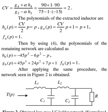
After applying the same procedure, the network seen in Figure 3 is obtained.
T(p)
L1 L2
C2 C1
Figure 3. Obtained high-pass LC ladder network
(Normalized element values: 1 , 8 , 7 , 4 , 5 1 2 2 1 L C L R C ).
4.3. Band-pass case
The following transfer scattering matrix is given for a band-pass LC ladder network,
) ( ) ( ) ( ) ( ) ( 1 ) ( p g p h p h p g p f p T where 1 2 26 30 120 ) (p p4 p3 p2 p h
,
1 8 56 90 120 ) (p p4 p3 p2 p g,
2 ) (p p f .
1 1 1 0 0 g h . Since
1, the first block is a series connected series-LC resonance circuit, and its element values are4 30 1 90 120 1 120 1 1 np np np np h g h g L , 5 1 1 1 ) 2 ( 1 8 0 0 1 1 h g h g C .
The polynomials of the extracted series inductor are p p CV p ha 2 2 ) ( , 1 2 1 2 ) (p CV p p ga , 1 ) (p fa .
Then by using (4), the polynomials of the remaining networks are calculated as
1 2 6 30 ) (p p3 p2 p hb , 1 8 36 30 ) (p p3 p2 p gb 2 ) (p p fb .
The polynomials of the extracted series capacitor are 10 1 2 1 ) ( CV p ha , 10 1 2 1 ) ( p CV p p ga and fa(p) p.
Then by using (4), the polynomials of the remaining network are calculated as
1 6 ) (p p2 hb
,
gb(p)6p26p1 p p fb( ).
After applying the same procedure, the network seen in Figure 4 is obtained.
Figure 4. Obtained band-pass LC ladder network (Normalized
element values: 1 , 2 , 3 , 5 , 4 1 2 2 1 C L C R L ).
4.4. Band-stop case
The following transfer scattering matrix is given for a band-stop LC ladder network,
) ( ) ( ) ( ) ( ) ( 1 ) ( p g p h p h p g p f p T where p p p p h( )24 36 2 2
,
1 4 54 60 252 ) (p p4 p3 p2 p g,
004 . 0 1905 . 0 ) (p p4 p2 f.
6 0 2h
1, so the first block is a shunt connected series-LC resonance circuit, and its element values are3 ) 24 ( 1 60 0 1 252 1 1 np np np np h g h g L , 2 0 1 1 2 1 4 0 0 1 1 h g h g C .
The polynomials of the extracted shunt connected series-LC resonance block are
p Cp p ha( ) 2 , 2 2 12 2 2 ) (p LCp2 Cp p2 p ga , 6 1 1 ) ( 2 p2 LC p p fa .
Then by using (4), the polynomials of the remaining network are calculated as
p p hb( )3
,
( ) 42 3 1 2 p p p gb,
42 1 ) (p p2 fb.
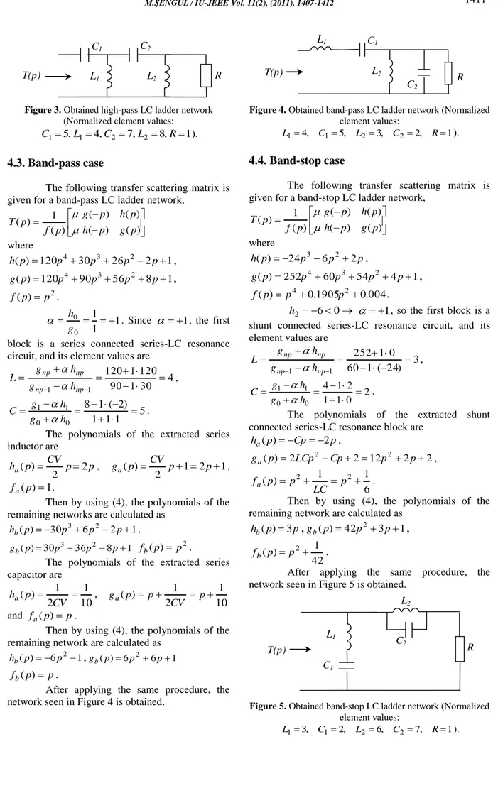
After applying the same procedure, the network seen in Figure 5 is obtained.
Figure 5. Obtained band-stop LC ladder network (Normalized
element values: 1 , 7 , 6 , 2 , 3 1 2 2 1 C L C R L ). T(p) L1 C2 C1 R L2 L2 C1 T(p) L1 C2 R L1 C 2 T(p) L2 C1 R
5. Conclusions
In this paper, an element value calculation algorithm has been proposed for LC ladder networks. It is based on the decomposition of transfer scattering matrix. Firstly the type and value of the element that will be extracted is obtained. Then after obtaining transfer scattering matrix of this element, transfer scattering matrix of the remaining network is calculated. The same procedure is applied until getting the termination resistance. Since all calculations are implemented in terms of the coefficients of the polynomials g(p),h(p),f(p), there is no need any root-search routines to get degree reduction after an element is extracted. As a result, an alternative element value calculation method for LC ladder networks is presented.
6. References
[1] N. Balabanian, “Network Synthesis”, Prentice-Hall, New Jersey, 1958.
[2] W. C. Yengst, “Procedures of Modern Network Synthesis”, The Macmillian Company, New York, 1964. [3] D. M. Pozar, “Microwave Engineering”, 3rd
ed., John Wiley & Sons, Inc., 2005.
[4] A. Aksen. “Design of lossless two-port with mixed lumped and distributed elements for broadband matching”, Ph.D. dissertation, Ruhr University, Bochum, Germany, 1994.
[5] L. Weinberg, P. Slepian, “Takahasi’s results on Chebysheff and Butterworth ladder networks”, IRE Trans. Circuit Theory, vol. CT-7, pp. 88-101, Jun. 1960. [6] R. Srinivasagopolan, B. A. Shenoi, “Necessary and
sufficient conditions on the poles and zeros of the reflection coefficient for low-pass ladder networks”, IEEE Trans. Circuit Theory, vol. CT-18, pp. 247-254, Mar. 1971.
[7] P. A. Mariotto, “On the explicit formulas for the elements in low-pass ladder filters”, IEEE Trans. Circuit Syst., vol. CAS-37, pp. 1429-1436, Nov. 1990.
[8] D. C. Fielder, “Numerical determination of cascaded LC network elements from return loss coefficients”, IRE Trans. Circuit Theory, vol. CT-5, pp. 356-359, Dec. 1958.
[9] H. J. Orchand, “Some explicit formulas for the components in low-pass ladder networks”, IEEE Trans. Circuit Theory, vol. CT-17, pp. 612-616, Nov. 1970. [10] S. Parker, P. Chirlian, E. Peskin,” Continuants and the
Synthesis of Low-Pass Resistively Terminated LC Ladder Networks”, IEEE Trans. Circuit Theory, vol. 13(2), pp. 209-212, Jun. 1966.
[11] M. Şengül, “Synthesis of cascaded lossless commensurate lines”, IEEE Trans. CAS-II: Express Briefs, vol. 55(1), pp. 89-91, Jan. 2008.
[12] M. Şengül, Z. Aydogar, “Transfer matrix factorization based synthesis of resistively terminated LC ladder networks”, Int. Conf. Electrical and Electronics Engineering, Eleco 2009, vol. II, pp. 74-77, Bursa, Turkey.
[13] M. Şengül, Z. Aydogar, “Synthesis of resistively terminated high-pass LC ladder networks”, Nat. Conf. Electrical and Electronics Engineering, Eleco 2010, vol. II, pp. 1-4, Bursa, Turkey.
[14] M. Şengül, “Circuit models with mixed lumped and distributed elements for passive one-port devices”,, Ph.D. dissertation, Işık University, İstanbul, Turkey, 2006.
[15] H. J. Carlin, P. P. Civalleri, “Wideband Circuit Design”, CRC Press LLC, 1998.
[16] A. Fettweis, “Factorization of transfer matrices of lossless two-ports”, IEEE Trans. Circuit Theory, vol. 17, pp. 86-94, Feb. 1970.
[17] A. Fettweis, “Cascade synthesis of lossless two-ports by transfer matrix factorization”, in R.Boite, ed., Network Theory, Gordon & Breach, pp. 43-103, 1972.
Metin ŞENGÜL received his B.Sc. and M.Sc. degrees in Electronics Engineering from Istanbul University, Turkey in 1996 and 1999, respectively. He completed his Ph.D. in 2006 at Işık University in Istanbul, Turkey. He worked as a technician at Istanbul University from 1990 to 1997 and was a circuit design engineer at the R&D Labs of the Prime Ministry Office of Turkey between 1997 and 2000. He was employed as a lecturer and assistant professor at Kadir Has University, Istanbul, Turkey between 2000 and 2010. Dr. Şengül was a visiting researcher at the Institute for Information Technology, Technische Universität Ilmenau, Ilmenau, Germany in 2006 for six months. Currently, he is an associate professor at Kadir Has University, Istanbul, Turkey and working on microwave matching networks/amplifiers, device modeling, circuit design via modeling and network synthesis.