An overview of design and operational issues of kanban systems M. S. AKTURK{* and F. ERHUN{
We present a literature review and classi® cation of techniques to determine both the design parameters and kanban sequences for just-in-time manufacturing systems. We summarize the model structures, decision variables, performance measures and assumptions in a tabular format. It is important to state that there is a signi® cant relationship between the design parameters, such as the number of kanbans and kanban sizes, and the scheduling decisions in a multi-item, multi-stage, multi-horizon kanban system. An experimental design is devel-oped to evaluate the impact of operational issues, such as sequencing rules and actual lead times on the design parameters.
1. Introduction
In recent years, the term just-in-time (JIT) has become a common term in repetitive manufacturing. It is used to describe a management philosophy that encourages change and improvement through inventory reduction. JIT can be de® ned as the ideal of having the necessary amount of material available where it is needed and when it is needed. It is an attempt to produce items in the smallest possible quantities, with minimal waste of human and natural resources, and only when they are needed. JIT systems have proven to be e ective at meeting production goals in environments with high process reliability, low setup times and low demand variability (Groenevelt 1993). In general, JIT has a pull system of coordination between stages of production. In a pull system, a production activity at a stage is initiated to replace a part used by the succeeding stage, whereas in a push system, production takes place for future need.
The advantages of JIT production include reduced inventories, reduced lead times, higher quality, reduced scrap and rework rates, ability to keep schedules, increased ¯ exibility, easier automation, and better utilization of workers and equip-ment. However, there is a limit to the extent that JIT can be usefully applied in many industries. The major JIT successes are in repetitive manufacturing environments. If the demand cannot be predicted accurately and product variety cannot be con-strained, it may not be possible to implement JIT e ectively. The ® nal assembly schedule must also be very level and stable. In pull approaches, information ¯ ow is tied to material ¯ ow, hence valuable information (e. g. on the demand trend) is not sent to all stages of production as soon as it is available. Pull systems can therefore
International Journal of Production Research ISSN 0020± 7543 print/ISSN 1366± 588X online#1999 Taylor & Francis Ltd
http://www.tandf.co.uk/JNLS/prs.htm http://www.taylorandfrancis.com/JNLS/prs.htm
Revision received August 1998.
{Department of Industrial Engineering, Bilkent University, 06533 Bilkent, Ankara,
Turkey.
be characterized by large information lead times, especially where there are large material ¯ ow times.
One of the major elements of JIT philosophy and pull mechanism is the kanban system. Kanban is the Japanese word for visual record or card. In a kanban system, cards are used to authorize production or transportation of a given amount of material. This system is the information processing and hence shop-¯ oor control system of JIT philosophy. While kanbans are being used to pull the parts, they are also used to visualize and control in-process inventories. The system e ectively limits the amount of in-process inventories, and it coordinates production and transporta-tion of consecutive stages of productransporta-tion in assembly-like fashion. Therefore, a kanban system is the manual method of harmoniously controlling production and inventory quantities within the plant. The kanban system appears to be best suited for discrete part production feeding an assembly line.
Kanban system can be either dual-card or single-card. The dual-card kanban system employs two types of kanban cards: production kanban and transportation (also called conveyance or withdrawal) kanban. A transportation kanban de® nes the quantity that the succeeding stage should withdraw from the preceding stage. A production kanban, on the other hand, de® nes the quantity of the speci® c part that the producing stage should manufacture in order to replace those which have been removed (Groenevelt 1993). Even though the dual-card kanban system pro-vides strong control on the production system due to its strict assumptions and prerequisites, such as design of the manufacturing system, smoothing of production and standardization of operations, it is di cult to implement it. Therefore, a variant of this system, called single-card kanban system, is sometimes used as a ® rst stage to develop a dual-card kanban system. In single-card kanban system, the transporta-tion of materials is still controlled by transportatransporta-tion kanbans. However, a produc-tion schedule provided by the central producproduc-tion planning is used to control the production within a cell instead of the production kanbans. Hence the system has a strong similarity to a conventional push system, with pull elements added to coor-dinate the transportation of the parts. One of the advantages of single-card push-pull system is its simplicity in implementation. Moreover, as the information on demand trend is sent to all stages of production as soon as its available, single-card kanban system has shorter information lead times compared to dual-card kanban systems. On the other hand, single-card kanban systems can also be used when the succeeding stage is physically close to its predecessor. In this case, the transportation kanban is eliminated and containers are moved at a time as needed. Only production kanbans are used. In this study, we use the former de® nition of a single-card kanban system, where the transportation of materials between the di erent workcentres is controlled by transportation kanbans.
Kanban system can be either instantaneous or periodic review system. In instan-taneous review systems, the kanbans are dispatched upstream as soon as an order occurs. In periodic review systems, the kanbans are collected and dispatched per-iodically. Periodic review systems may be either ® xed quantity, non-constant with-drawal cycle, or ® xed withwith-drawal cycle, non-constant quantity (Monden 1993). Under the ® xed quantity, non-constant withdrawal cycle system, kanbans are dis-patched upstream when the number of kanbans posted on a withdrawal kanban post reaches a predetermined order point. Under the ® xed withdrawal cycle, non-constant quantity system, the period between material handling operations is ® xed and the quantity ordered depends on the usage over the withdrawal cycle.
2. Literature review
We ® rst provide a comparative review of kanban literature on determining the design parameters using a tabular format, then discuss the studies on determining the kanban sequences to show the impact of operational issues on the design parameters. 2.1. Determining the design parameters
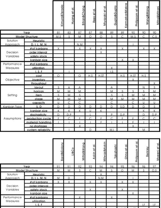
In this section, we review the models for determining the design parameters in a kanban system, and summarize the model structures, decision variables, perform-ance measures and assumptions in a tabular format. The characteristics considered in this review are classi® ed as follows (the emboldened letters give the key to the entries in table 1 later):
1. Model structure: Mathematical programming, Simulation, Markov Chains, Others
2. Solution approach: 2.1. Heuristic
2.2. Exact: Dynamic programming, Integer programming, Linear program-ming,Mixed integer programming, Nonlinear integer programming. 3. Decision variables:
3.1. Number of kanbans 3.2. Order interval 3.3. Safety stock level 3.4. Kanban size 4. Performance measures:
4.1. Number of kanbans 4.2. Utilization
4.3. Measures:Inventory holding cost,Shortage cost, Fill rate 5. Objective:
5.1. Minimize cost: InventoryHolding cost,Operating costs, Shortage cost, SeTup cost.
5.2. Minimize inventory 5.3. Maximize throughput 6. Setting:
6.1. Layout : Assembly-tree,Serial,Network without backtracking 6.2. Time period:Multi-period,Single-period
6.3. Item: Multi-item, Single-item 6.4. Stage: Multi-stage, Single-stage 6.5. Capacity: Capacitated, Uncapacitated
7. Kanban type: Single-card kanban,Dual-card kanban 8. Assumptions:
8.1. Kanban sizes: Known,Unit
8.2. Stochasticity: Demand,Lead time, Processing time,Setup time 8.3. Production cycle:Fixed production intervals, Continuous production 8.4. Material handling: Fixed withdrawal cycle,Instantaneous
8.5. No shortages
8.6. System Reliability:Dynamic demand,Machine unreliability,Imbalance between stages, Rework
Most of the existing studies in the literature are modelled by using a mathemat-ical programming, Markov chain or simulation approaches. There are a few excep-tional studies that use other methods such as statistical analysis or the Toyota formula. In table 1 later, we collect these models under the heading `others’. On the other hand, a solution approach can be either heuristic or exact. For an exact solution methodology, one of the dynamic programming, integer programming, linear programming, mixed integer programming, or nonlinear integer programming techniques can be used to ® nd an optimum solution.
For the analytical models the decision variables are mainly kanban sizes, number of kanbans, withdrawal cycle length for periodic review models, and safety stock levels. For the simulation models the commonly used performance measures are number of kanbans, machine utilizations, inventory holding cost, backorder cost, and ® ll rates. Fill rate can be de® ned as the probability that an order will be satis® ed through inventory. Models can consider di erent combinations of the criteria stated above. The objectives for the analytical models can be minimizing the costs or minimizing the inventories. For the cost minimization, the cost terms can be con-sidered either independently as inventory holding cost, shortage cost, and setup cost, or the combination of these costs as an operating cost. Another objective for stoch-astic models can be maximizing the throughput of the system.
The production setting for the models include the layout, number of time peri-ods, number of items, number of stages, and capacity. Layout can be serial (¯ ow-line), assembly-tree, or a general network without backtracking (modi® ed ¯ owline). An empty cell in the table for any of these indicate that the characteristic is not considered in the corresponding study.
Kanban system can be either a single-card or a dual-card. The assumptions for the models are also stated in the tabular format. These assumptions are the ones that are commonly considered, more speci® c ones are indicated in the explanations of the models. The ® rst assumption is on the kanban size. An empty cell for this character-istic indicates that the kanban size is not a parameter, but is a decision variable for the system. Another assumption relates to the nature of the system such that the system can be either stochastic or deterministic. For the deterministic models, this cell is left empty. For the stochastic ones, the stochastic parameters are indicated. The production cycle di erentiates between the models that have continuous pro-duction and ® xed propro-duction intervals. The fourth assumption speci® es the material handling mechanism, and it can be either an instantaneous or a periodic one. The ® fth assumption is related to backorders. An empty cell indicates that backorder is allowed. And, the last assumption is on the system reliability. If the system is re-liable, this cell is left empty, otherwise the unreliability of the system is stated. In table 1, the models are presented using the classi® cation scheme listed at the start of § 2.1. Further explanations of the models are given below.
Kimura and Terada (1981) describe the operation of kanban systems and ex-amine the accompanying inventory ¯ uctuations in a JIT environment. They provide several balance equations for kanban systems in a single item, multi-stage, uncapa-citated serial production setting to demonstrate how demand ¯ uctuations of the ® nal product in¯ uence the ¯ uctuations of production and inventory at the upstream stages. The authors use simulation to show that ¯ uctuations are ampli® ed when the size of order and/or lead time becomes large.
Huang et al. (1983) simulate the JIT with kanban for a multi-line, multi-stage production system in order to determine its adaptability to a US production
envir-Ki m ur a& Te ra da Hu an g et a l. Bi tra n& C ha ng Re es e t a l. M iy az ak i e t a l. G up ta &G up ta Ka rm ar ka r& Ke kr e Ph ilip oo m e t a l. W an g& W an g M itr a& M itr an i Year 81 83 87 87 88 89 89 90 90 90 Model Structure M,S S M O O S C M,S C C,S Solution Heuristic A pproach D, I, L, M, N N,M I # of kanbans X X X X X X X
Decision order interval X
Variables safety stock
kanban size X X Performance # of kanbans Measures utilization X I, S, F I I,S cost O O H,S H,ST H,S H,ST H,S Objective inventory X throughput X layout S A A A N S horizon M M M M S S S M Setting item S M S S S M M M stage M M M M M M M M capacity U C C C C U U Kanban Type S, D D D D D D D S,D D D S kanban size K K K U K K K stochasticity D D,P L P D,P D D,P
Assumptions production cycle F C F C F C F F C C
material handling I I I I F I I F I I
no shortages X X
system reliability I D M,I M
Ba rd &G ol on y Li& C o M itt al &W an g A sk in e t a l. M itw as i& A sk in Ta ka ha sh i O hn o et a l. Ph ilip oo m e t a l. Be rk le y M oe en i e t a l. Y ear 91 91 92 93 94 94 95 96 96 97
Model Structure M M S C M S O M S O,S
Solution Heuristic X
A pproach D, I, L, M, N M D N,M I
# of kanbans X X X X X X
Decision order interval
V ariables safety stock X X
kanban size X Performance # of kanbans X X Measures utilization I, S, F I,F I,F cost S,H,ST H H,S O H,S,ST H,ST Objective inventory throughput layout A S,A N S S A S S horizon M M M S M M M M M M Setting item M S M M M S S M M S stage M M M M S M S M M M capacity C U C C C C Kanban Type S, D S D D S D D D D D S kanban size K K K K K K U K stochasticity D,P D,P D,P D D,P D,P,S
A ssumptions production cycle F F F F C F F C F
material handling I I I I I I I I I I
no shortages X X X
system reliability M,R D I M
onment. The simulated production system includes variable processing times (nor-mally distributed), variable master production scheduling (exponentially distributed demand), and imbalances between production stages. The authors conclude that the variability in processing times and demand rates are ampli® ed in a multi-stage set-ting, and that excess capacity has to be available to avoid bottlenecks. Monden (1984) comments on the conclusion drawn by Huang et al. (1983). He stated that the kanban system should be able to adapt to daily changes in demand within 10% deviations from the monthly master production schedule (MPS). Larger seasonal ¯ uctuations in demand can be accommodated by setting up the monthly MPS appropriately.
Bitran and Chang (1987) extend Kimura and Terada’s (1981) serial model. They provide a nonlinear integer formulation for kanban systems in a deterministic, single item, multi-stage, capacitated, assembly-tree structure production setting. The for-mulation assumes zero transportation lead time and planning periods of known length, and ® nds the minimum feasible number of kanbans. The authors show that the initial nonlinear model can be transformed into an integer linear program with the same feasible and optimal solutions. The proposed model does not incor-porate uncertainties.
Rees et al. (1987) develop a methodology for dynamically adjusting the number of kanbans in an unstable production environment. They use the Toyota equation with unit kanban capacities, forecasted demands and estimates of kanban lead time probability density functions to determine the number of kanbans.
Miyazaki et al. (1988) modify the conventional economic order quantity model to determine the average inventory for ® xed interval withdrawal and supplier kanban systems, give formulae to determine the minimum number of kanbans required, and derive an algorithm to obtain the optimal order interval. The objective is to minimize the average inventory holding and ordering costs in a deterministic setting.
Gupta and Gupta (1989) simulate a single item, multi-line, multi-stage, dual-card kanban system. They investigate the impact of changing the number of kanbans and kanban sizes on the performance of the system. The performance measures are chosen to be in-process inventory, capacity utilization or production idle time, and shortage of the ® nal product. The authors conclude that determining the number of kanbans is essential to the performance of the system, and keeping the bu er size constant by increasing the kanban size and decreasing the number of kanbans accordingly increase the inventory. For the smooth operation in a JIT environment the stages should be balanced and the suppliers should be reliable. Finally, the system performance declines with an increase in demand variability.
Karmarkar and Kekre (1989) develop a continuous time Markov model to study the e ect of batch sizing policy on production lead time and inventory levels. Both single and dual card kanban cells and two-stage systems are modelled. They also examine the e ect of varying the number of kanbans in the cell. The primary intent of the investigation is to develop a qualitative analysis of kanban systems that can provide insights to parametric behavior of kanban systems. The results show that the kanban size has a signi® cant e ect on the performance of kanban systems.
Philipoom et al. (1990) describe the signal kanban technique and demonstrate two versions of an integer mathematical programming approach for determining the optimal lot sizes to signal kanbans in a multi-item, multi-stage setting. A simulation model is employed to test the e ectiveness of the programming models. The models
assume no backorders, therefore the stages are decoupled and interdependencies are eliminated.
Wang and Wang (1990) present a continuous time Markov model to determine the number of kanbans in a multi-item, multi-stage, dual-card kanban system with a single withdrawal kanban for each stage. The model can be applied to serial, as-sembly (merge) type and disasas-sembly (split) type production settings. The authors assume that the production and demand rates are exponential. Furthermore, the stages are assumed to be independent. To determine the number of kanbans, several alternatives for number of kanbans are considered, and the one with minimum cost is chosen. The model can be extended to systems with unreliable machines.
Mitra and Mitrani (1990) present a continuous time Markov model for a multi-item, multi-stage, serial production setting. The processing times are exponentially distributed and the raw material and demand arrival have Poisson distribution. The authors show the equivalence of kanban system to the tandem sequence with mini-mal blocking policy. They also show that, under their distribution assumptions, the throughput-inventory relation of kanban system dominates that of traditional dis-cipline of manufacturing blocking. The authors develop an approximation algor-ithm, which is compared with a simulation model. As a result, they observe that the approximation has the largest errors in the long production lines with few kanban cards in each cell. The model can be extended to systems with unreliable machines. Bard and Golony (1991) develop a mixed integer linear program to determine the number of kanbans at each stage in a multi-item, multi-stage, capacitated, general assembly shop. The objective is to minimize inventory holding, shortage and setup costs for a given demand and planning horizon without violating the basic kanban principles. The model is most appropriate when the demand is steady and the lead times are short.
Li and Co (1991) extend Bitran and Chang’s (1987) model to develop bounds for an e cient kanban assignment and apply them to solve a dynamic programming model in a deterministic, single item, multi-stage, serial/assembly-tree structure pro-duction setting. The authors assume an in® nite capacity. This assumption not only removes the capacity constraints but also eliminates the need to keep track of the number of units in partially ® lled kanbans. Therefore, the model is computationally very e cient, even for a complex non-serial system.
Mittal and Wang (1992) develop a database-oriented simulator, called CADOK (computer aided determination of kanbans), to determine the number of kanbans in a production setting where breakdowns, reworks, setup times, variable processing times (normally distributed), and variable demand (exponentially distributed) are modelled. Backorder costs are assumed to be prohibitively high. The model can handle both assembly and disassembly type operations such that several stages supply products to the same stage or one stage supplies parts to several stages. Furthermore, delay can be induced for the information to travel from one stage to another. However, the system cannot handle backtracking so it is only applicable to ¯ owlines or modi® ed ¯ owlines.
Askin et al. (1993) develop a continuous time, steady-state Markov model for determining the optimal number of production kanbans in a multi-item, multi-stage, serial production setting. The objective is to minimize the inventory holding and shortage costs given external demand and the kanban sizes. The external demand assumption permits the modelling of a multi-stage system as independent stages. The model uses the Toyota equation, and ® nds the number of kanbans and safety factor.
The performance of the model is sensitive to the accurate estimation of the queue lengths.
Mitwasi and Askin (1994) provide a nonlinear integer mathematical model for the multi-item, single stage, capacitated kanban system. It is assumed that demand is external, dynamic and evenly distributed over period, the system is reliable, setups are small enough to allow batch sizes as small as a single kanban, and no shortages are permissible. The control periods are assumed to be small enough to ignore batch sequencing problem. The model is transformed to a simpler model with the same set of optimal and feasible kanban solutions. Lower and upper bounds for the number of kanbans are developed. A heuristic solution is also presented.
Takahashi (1994) provides a simulation model to determine the number of kanbans for a single item, unbalanced serial production systems under stochastic conditions (demand with exponential distribution and processing time with gamma distribution). An algorithm that allows di erent numbers of production and with-drawal kanbans at an inventory point is proposed. It is assumed that the total number of kanbans are known, withdrawal lead time is negligible, and backorders are allowed.
Ohno et al. (1995) derive the stability condition of a JIT production system with the production and supplier kanbans under the stochastic demand and deterministic processing times. An algorithm for determining the optimal number of two kinds of kanbans that minimize an expected average cost per period is devised. In other words, this algorithm determines the optimal safety stocks in the Toyota equation. Philipoom et al. (1996) provide a nonlinear integer mathematical model for the multi-item, multi-stage, multi-period, capacitated kanban system. It is assumed that demand is deterministic, the system is reliable, setups are sequence-independent, production costs are stable, lot sizes remain constant throughout the shop and no shortages are permissible. The model determines the kanban sizes, number of kan-bans, and ® nal assembly sequence simultaneously by minimizing the setup and inventory holding costs.
Berkley (1996) investigates the e ect of kanban size on system performance in a multi-item, multi-stage, dual-card kanban system. The performance measures are in-process inventory and customer service level. The author varies the number of kan-bans and kanban sizes in the tandem so that the total in-process inventory capacity remains constant. Simulation results show that smaller kanban sizes lead to smaller in-process inventories, and smaller kanban sizes can lead to better customer service when the cost of the greater setup times can be o set by the bene® ts of more frequent material handling. The study assumes that the kanban sizes and number of kanbans are same for all parts and the set of kanban size values are independent of the demand distribution.
Moeeni et al. (1997) propose a methodology, based on Taguchi’s robust design framework, to implement kanban systems in uncertain production environments. The authors model the e ects of environmental variations such as demand patterns, supplier lead times, setup times, processing times, time between breakdowns and repair times on the kanban system performance. To evaluate the performance of design, they use a quadratic loss function. The proposed methodology is examined via simulation. An experimental design that considers the number of kanbans, kanban review periods and container sizes simultaneously is performed. The authors ® nd that for their system, the container size is the most important factor in terms of the performance measures used.
The current literature can be extended in several ways. For each part in the Kanban system two basic design parameters have to be determined: the kanban size, and the number of kanbans to be used. Very few studies exist that consider the kanban sizes explicitly, i.e. Gupta and Gupta (1989), Karmarkar and Kekre (1989), Philipoom et al. (1996), and Moeeni et al. (1997). Berkley (1996) studies the e ect of kanban sizes on system performance, but he assumes that the kanban sizes are set regardless of the demand distribution. Most of the models assume that the kanban sizes are known and the number of kanbans can be determined by using these predetermined values. In fact, the number of kanbans and kanban sizes should be determined simultaneously, as these two together a ect the performance of the system. Almost none of the models, except Philipoom et al. (1996), consider the impact of operating issues on design parameters. It is usually assumed that the control periods are small enough to ignore the batch sequencing problem. Even in the study of Philipoom et al., only the ® nal assembly sequence is determined and it is assumed that it propagates back by the ® rst-come-® rst-served (FCFS) rule. In gen-eral, instantaneous material handling is used. There are only two models that use non-instantaneous material handling, by Miyazaki et al. (1988) for supplier and withdrawal kanbans, and by Philipoom et al. (1990) for signal kanbans. The model structures are di erent, and their ® ndings cannot be generalized to a dual-card kanban system.
Several models in the literature assume station independence. Askin et al. (1993) and Mitwasi and Askin (1994) assume external demand. The demand for each stage is externally generated and with the assumption of su cient capacity, the multi-stage system can be modelled as independent stages linked by their proportional demand rates. Kimura and Terada (1981), Philipoom et al. (1990), and Li and Co (1991) assume that the capacity is unlimited. Bitran and Chang (1987), Philipoom et al. (1990) and Philipoom et al. (1996) do not allow backorders. Under JIT system, all stages are integrally tied to each other and if there is a delay in one stage then both the preceding and succeeding stages should be a ected to highlight interdependencies among the stages. This is crucial for reducing the size of the inventory levels and eliminating overall waste. Although this possibility is eliminated with the assumption of no backorders and an in® nite production capacity, hence each stage can be modelled independently.
2.2. Determining the kanban sequences
In JIT systems, the ® nal assembly schedule determines production orders for all of the stages in the facility. Once the assembly line is scheduled, it is assumed that the sequence propagates back through the system. Kanbans in the rest of the shop are processed in order in which they are received, i.e. FCFS. However, there are several studies in the literature that test this assumption.
Lee (1987) compares the FCFS, shortest processing time (SPT), SPT/LATE, higher pull demand (HPF), and HPF/LATE in a ¯ ow shop using a dual-card kanban system with ® xed order points. Simulation results show that the SPT and SPT/LATE rules outperform others in several performance measures considered such as production rate, utilization, queue time, and tardiness. The same system is simulated to see the e ect of di erent job mixes, pull rates, and number of kanbans and kanban sizes on the system performance.
Berkley and Kiran (1991) compare the performance of SPT, FCFS, SPT/LATE, and FCFS/SPT rules in a dual-card kanban system with constant withdrawal cycles.
They modify the SPT/LATE used by Lee (1987) to use the local information. They ® nd that contrary to the conventional results, the SPT rule creates the largest average output material queues and in-process inventories, and the FCFS and FCFS/SPT create the least and outperform other two rules. Berkley (1993) compares the per-formance of FCFS and SPT in a single-card Kanban system with varying queue capacities and material handling frequencies by a simulation model. He is shown that the results of Berkley and Kiran (1991) are due to material handling mechanism used in both of the models since it favors the FCFS rule which maintains consistent kanban priorities from stage to stage and prevents kanban passing.
Lummus (1995) simulates a JIT system to investigate the e ect of sequencing on the performance of the system in a multi-item, multi-stage, assembly-tree structure setting. The author uses three sequencing rules, which are Toyota’s goal chasing algorithm (a detailed explanation of the algorithm can be found in Monden 1993), demand-driven production and producing all the jobs of the same kind, and study their e ects for di erent sequences given various setup and processing times. She concludes that the sequencing method selected a ects the performance of the system. The problem of production levelling through scheduling is crucial to kanban systems. Sequencing in kanban-controlled shops are more complex compared with conventional sequencing problems, as the kanbans may not have speci® c due dates and kanban-controlled shops can have station blocking (Berkley 1992). Station blocking can be described as the idleness of a stage due to full out-bound inventories. Although there are several studies on kanban scheduling, the rules used in these studies are simple dispatching rules. More sophisticated scheduling rules should be used to determine the e ects of scheduling on the performance of kanban systems. Detailed reviews of JIT and kanban systems can be found in Berkley (1992), Groenevelt (1993), and Huang and Kusiak (1996).
3. Computational analysis
As pointed out above, there is a close interaction between the design parameters of kanban systems, i.e. the number of kanbans and the kanban sizes, and the kanban sequences. Furthermore, Savsar (1996) showed that kanban withdrawal policies might a ect throughput rate and inventory levels of JIT production control systems. Therefore, we develop an experimental design to determine the withdrawal cycle length, number of kanbans, kanban sizes and kanban sequences at each stage simul-taneously for a periodic review multi-item, multi-stage, multi-period kanban system under di erent experimental conditions. The overall objective is to minimize the total production cost, which is comprised of backorder and inventory holding costs. The inventory holding cost and backorder cost are the sum of the inventory holding and backorder costs over all stages, respectively.
Another important question is to investigate the impact of operating issues such as sequencing rules and actual lead times on the design parameters. In order to ® nd the kanban sequences at each stage, four sequencing rules commonly used in the literature are considered, which are SPT, SPT-F, FCFS, and FCFS-F. For each rule, the selection is made among the items on the schedule board that have a correspond-ing full kanban in in-bound storage. It is shown by Berkley and Kiran (1991) that under periodic review kanban systems, FCFS and FCFS/SPT rules perform better than SPT or SPT/LATE. Lee (1987) and Lee and Seah (1988), on the other hand, show that SPT and SPT/LATE perform better than the FCFS rule. As discussed earlier, the assumptions of these studies, especially material handling mechanisms
used in both of the simulation models, were di erent. Berkley and Kiran’s model favors the FCFS rule since it maintains consistent kanban priorities from stage to stage and prevents kanban passing. Therefore, we select FCFS and SPT/LATE as in the earlier studies their performance are justi® ed. WemmerloÈv and Vakharia (1991) show that the family-based rules perform better than their corresponding item-based rules when the performance measure is ¯ ow time. Therefore, even though the family-based rules have not been used in JIT literature before, we select the corresponding family-based rules of FCFS and SPT/LATE to test the validity of this ® nding under kanban setting. Hence, when multiple kanbans are waiting, by combining the pro-duction runs for several kanbans a temporary increase in throughput can be achieved by eliminating some setups. The algorithms for these rules are given below, and the notation used throughout the experimental design are as follows:
aTij the kanban size for item…i;j†for the withdrawal cycle length of T bijm unit backorder cost of item…i;j†at stage m
Dtijm demand for item…i;j†at stage m in period t (number of kanbans)
hijm unit inventory holding cost of item…i;j†at stage m
MINVijm the maximum inventory level of item…i;j†at stage m
MSijm maximum absolute delay of item…i;j†at stage m nT
ij the number of kanbans for item…i;j†for the withdrawal cycle length of T
pijm processing time of item…i;j†at stage m size‰iŠ number of parts in family i
Qijm‰sŠ number of kanbans of item…i;j†at stage m that are backlogged for s periods
Algorithm 1 Ð for FCFS:
Step 1. Update the delay values for each item, where, delay is de® ned as the di er-ence between the arrival time of the item and the current time.
Step 2. Of the unscheduled items select the item with maximum absolute delay. If ties exist, use the SPT as the tie-breaking rule.
Algorithm 2 Ð for FCFS-F:
Step 1. Calculate the total backorders of each family: total backorder of family iˆ X
size‰iŠ jˆ1 X MSijm sˆ1 s Qijm‰sŠaTij:
Step 2. Of the unscheduled families, select the family with maximum total back-order. Schedule all the items in the family with the FCFS. In case ties exist in the family selection, use the SPT-F as the tie-breaking rule. Algorithm 3 Ð for SPT/LATE:
Step 1. Update the delays of each item. If the maximum absolute delay is smaller than the predetermined level:
Step 1.1. Calculate the updated processing time for each item: puijmˆ setup time for family i‡ pijmDtijmaTij
Step 1.2. Of the unscheduled items, select the item with minimum updated processing time. If ties exist, use the FCFS as the tie-breaking rule. Step 2. Else, use the FCFS to schedule the items.
Algorithm 4 Ð for SPT-F:
Step 1. Calculate the average processing time of each family: average processing
time of f amily iˆ
setup time for family i‡ X
size‰iŠ
jˆ1
pijmDtijmaTij
size‰iŠ :
Step 2. Of the unscheduled families, select the family with minimum average pro-cessing time. In case ties exist, use the FCFS-F as the tie-breaking rule. There are seven experimental factors that can a ect the e ciency of kanban systems. The parts that share the same setup, processing and routing requirements are grouped into the part families. A more detailed discussion on the formation of part families and corresponding manufacturing cells can be found in Akturk and Balkose (1996). Therefore, the number of families and the number of parts in each family, i.e. factors A and B, a ect the product mix and congestion of the shop ¯ oor. As the number of families increase, the setup requirement increases and the sched-uling decision becomes more important. The demand for each part is stochastic but comes from ® ve di erent scenarios. In each scenario, demand is uniformly distrib-uted. The probability mass function (PMF) of the demand distribution for the low-variability case is de® ned below where · is the average demand and UN ‰a;bŠ
represents a uniformly distributed random variable in the interval‰a;bŠ:
fD…d†ˆ 0:1; Dˆ UN ‰·¡ 10; ·¡ 7Š 0:2; Dˆ UN ‰·¡ 6; ·¡ 3Š 0:4; Dˆ UN ‰·¡ 2; ·‡1Š 0:2; Dˆ UN ‰·‡2; ·‡5Š 0:1; Dˆ UN ‰·‡6; ·‡9Š: 8 > > > > > > < > > > > > > :
This density states that 10% of the time demand will be distributed uniformly between‰·¡ 10; ·¡ 7Š, and for another 20% of the time it will be distributed uni-formly between‰·¡ 6; ·¡ 3Š, and so on. The PMF of the demand distribution for the high-variability case is de® ned as
fD…d†ˆ 0:1; Dˆ UN ‰·¡ 15; ·¡ 11Š 0:2; Dˆ UN ‰·¡ 10; ·¡ 6Š 0:4; Dˆ UN ‰·¡ 5; ·‡ 4Š 0:2; Dˆ UN ‰·‡ 5; ·‡ 9Š 0:1; Dˆ UN ‰·‡ 10; ·‡ 14Š 8 > > > > > > < > > > > > > :
The ® fth factor speci® es the relative load of each stage. In the balanced case, the processing times of items have the same uniform distribution at each stage. In the unbalanced case, the processing times at the fourth stage (stage D in the routing) has a uniform distribution with a higher mean. Therefore, the fourth stage becomes a bottleneck stage and consequently the smooth material ¯ ow is disturbed. The sixth factor is used to determine the sequence-dependent setup times at each stage. The setup time has a uniform distribution. The lower bound, SLm, and the upper bound, SHm, of the uniform distribution are calculated by using the S/P ratio and the pro-cessing times at each stage. First, the average propro-cessing time of each family at each stage is calculated as follows, where K is an estimated kanban size:
average processing time of family i at stage mˆ
X
size ‰iŠ
jˆ1
pijm K size‰iŠ :
The parameter K is selected according to factor B. K is equal to 25 or 50, when factor B is at the low or high level, respectively. These di erent values are used to keep the ratio of the setup time to total time constant. Then, SLmand SHmvalues are calculated as follows:
SLmˆ …S/P† (average processing time of family i at stage m) 0:50
SHmˆ …S/P† (average processing time of family i at stage m) 1:50:
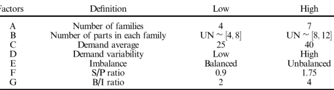
The seventh factor is the backorder cost to inventory holding cost B/I ratio. The backorder cost of an item is equal to the inventory holding cost times the B/I ratio such that bijmˆ …B/I†hijm. The experimental design is a 27 full-factorial design as
there are seven factors with two levels each, which are listed in table 2. Five replica-tions are taken for each combination, resulting in 640 di erent randomly generated runs.
Other variables in the system are treated as ® xed parameters and generated as follows:
. There are ® ve stages, denoted as A, B, C, D and E. The routings for families
are ® xed and are given in ® gure 1. When factor A is at the low level, the ® rst four families are used.
. The inventory holding costs are generated randomly from the interval
UN ‰5;10Š:
. The processing times for the balanced case are selected randomly from the
interval UN ‰0:1;0:3Š. For the unbalanced case, the processing times at
Factors De® nition Low High
A Number of families 4 7
B Number of parts in each family UN ‰4;8Š UN ‰8;12Š
C Demand average 25 40
D Demand variability Low High
E Imbalance Balanced Unbalanced
F S/P ratio 0.9 1.75
G B/I ratio 2 4
stage D are selected randomly from the interval UN ‰0:3;0:5Š when the
number of parts in each family are low, and from the interval UN ‰0:2;0:4Š when it is high. Two di erent distributions are selected to
keep the setup to processing time ratio in the system constant.
Kanban systems maintain constant levels of total on-hand and in-process inven-tory at each production stage. To determine the maximum inveninven-tory level, we use the Toyota formula:
maximum inventory levelˆ n aˆ D L…1‡ s†
where n is the number of kanbans, a is the kanban size, D is the average demand rate, L is the expected lead time, and s is the safety factor. The safety factor, s, is taken as 0.05. An important problem that arise with the Toyota formula is the estimation of the lead times. Lead time is not an attribute of the part, rather it is a property of the shop ¯ oor. Lead times vary greatly depending on capacity, shop load, product mix and batch sizes as discussed in Karmarkar (1993). For the lead time estimation, Ragatz and Mabert (1984) show that the rules that utilize shop information generally perform better than rules that utilize only job information. Therefore, we select the work-in-queue rule proposed by Ragatz and Mabert. As the lead times are estimated for each stage, the maximum inventory levels for an item at each stage will change. In that way, we can allocate di erent number of kanbans at each stage for the same item. This will not only increase the solution space for the scheduling but also may increase the power of the kanban system over imperfect settings (Takahashi 1994). Karmarkar and Kekre (1989) show that the e ects of kanban sizes, number of kanbans, and their interactions are signi® cant on the performance of kanban systems. Therefore, we vary the number of kanbans and kanban sizes in a way that the maximum inventory level for each part at each stage, MINVijm, remains constant. There are three decision variables that are the withdrawal cycle length, T , the number of kanbans for part i of family j, denoted as item…i;j†, for a given T , nTij, and the kanban sizes, aTij. For the withdrawal cycle length, six alternatives are gen-erated such asf8;4;2;1;0:5;0:25g hours orf480;240;120;60;30;15g minutes. We
also generate a set of number of kanbans as a power of 2, hence the alternative kanban sizes for each item are calculated as follows:
aTij ˆ MINVijm nT ij & ’ ; 8T and nTij ˆ f1;2;4;8;16;32g ( ) :
Therefore, to determine the values of the decision variables, each sequencing rule will evaluate 36 alternatives for each replication and ® nd the kanban sequences at each
4 2, 5, 6 1,4 1,2,3,4,5,6,7 1 1, 3 3, 7 2, 4, 6, 7 1, 3, 5 1, 3, 5 E D C B A
stage to select the alternative with the minimum sum of inventory holding and backorder costs.
There are six alternative T values and the number of instances of best T values for all runs are summarized in table 3. For the family-based methods, the setup to processing time ratio is smaller, therefore family-based methods can force the with-drawal cycle lengths to shorter values. This ratio is relatively higher for the FCFS rule, so longer withdrawal cycle lengths are chosen to minimize total production cost. When we analyse table 3, we see that the withdrawal cycle length selected is not robust to scheduling rule used. This result shows the impact of operating parameters on design parameters in decision making. In the existing literature, instantaneous material handling and FCFS are used together, although we can easily claim that this combination may not be e ective for all experimental conditions. In fact, item-based rules perform well when the withdrawal cycle lengths are long enough to justify the setup times and to highlight the items. The FCFS-F rule, on the other hand, prefers shorter withdrawal cycle lengths than the FCFS rule to minimize the under production of less desirable items since it cannot react timely to the demand variations due to long production of families.
The overall results of the di erent sequencing rules are summarized along with the minimum, average, and the maximum values in tables 4± 7. The maximum inven-tory levels of the rules, which are calculated by summing up the inveninven-tory holding costs when inventories are full over all stages over the planning horizon, are given in table 4. For the kanban system to work properly a minimum level of inventory should be kept in the system. Once this level is determined, the inventories should
T (min) FCFS FCFS-F SPT/LATE SPT-F 480 26 9 6 8 240 310 174 110 108 120 223 144 75 139 60 43 105 108 89 30 29 149 240 199 15 9 59 101 97
Table 3. Comparison of the number of instances of best withdrawal cycle lengths.
Maximum inventory level FCFS FCFS-F SPT/LATE SPT-F
Minimum 107 280 94 368 94 368 98 144
Average 1 686 037 1 319 805 954 144 1 068 906
Maximum 8 056 192 8 056 192 8 056 192 8 056 192
Table 4. Comparison of the maximum inventory levels of sequencing rules.
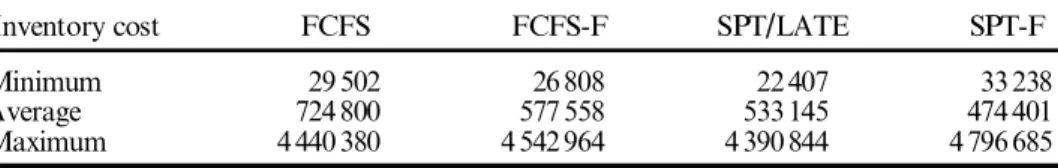
Inventory cost FCFS FCFS-F SPT/LATE SPT-F
Minimum 29 502 26 808 22 407 33 238
Average 724 800 577 558 533 145 474 401
Maximum 4 440 380 4 542 964 4 390 844 4 796 685
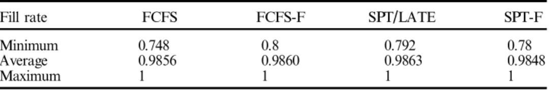
be kept full, and the deviations re¯ ect the nervousness of the system that should be interpreted as lost production. The maximum inventory level is not a performance measure and it should not be interpreted alone. As long as the system performs good, the lower the inventory level, the better the system performance. The minimum value is achieved by the SPT/LATE rule. Furthermore, there is a positive correlation between the withdrawal cycle length and the maximum inventory levels such that the maximum inventory level increases for the longer the withdrawal cycle lengths. Therefore, the FCFS rule gives the highest maximum inventory level value. The maximum value for all rules is occurred for the same factor combination of …1110111†, where low and high levels for each factor are represented by 0 and 1, respectively. In other words, all of the factors except the demand variability are at their high levels. For the inventory holding cost, the minimum average value is given by the SPT-F rule as shown in table 5. When we interpret these values in conjunction with the maximum inventory levels, we see that on the average 42.99%, 43.76% and 44.38% of inventories are full for FCFS, FCFS-F and SPT-F, respectively. The best performance is achieved by the SPT/LATE rule, as on the average 55.88% of inven-tories are full. These ® gures are obtained by dividing the average inventory holding cost to average maximum inventory level of each rule. These ratios also indicate that the system performance can be signi® cantly improved by using a more sophisticated scheduling algorithm. Table 6 shows the backorder costs for the sequencing rules. The best average performance is again achieved by the SPT/LATE rule. We also compare the ® ll rates of these rules as indicated in table 7. The ® ll rate is the probability of an order being satis® ed through the inventories and it is calculated only for the ® nal stage A. The relative performance of the rules is same as the one for the backorder cost. We applied a paired t-test to the cost terms of the 640 randomly
FCFS FCFS-F SPT/LATE SPT-F
Minimum total cost and minimum T 48 83 326 215
Minimum total cost but not minimum T 0 26 27 20
Table 8. Comparison of the best rules.
Fill rate FCFS FCFS-F SPT/LATE SPT-F
Minimum 0.748 0.8 0.792 0.78
Average 0.9856 0.9860 0.9863 0.9848
Maximum 1 1 1 1
Table 7. Comparison of the ® ll rates of sequencing rules.
Backorder cost FCFS FCFS-F SPT/LATE SPT-F
Minimum 9118 0 0 0
Average 1 756 864 1 098 431 855918 1 155 939
Maximum 7 115 735 5 851 782 5 888825 7 377 613
generated runs found by these sequencing rules to check the statistical signi® cance of their di erences. For the inventory holding cost, the rules were statistically di erent with p40:000 signi® cance, except the FCFS-F and SPT/LATE pair for which
p40:002. For the backorder cost, all of the rules were again di erent with
p40:000 signi® cance, except the FCFS-F and SPT-F pair for which p40:005. In
table 8, we summarize the number of times the minimum total cost value of a sequencing rule outperforms others over 640 runs. Notice that more than one sequencing rule can have the best value for a certain run if there is a tie. Furthermore, a sequencing rule that ® nds the minimum total cost may not necess-arily give the minimum T value as shown in table 8.
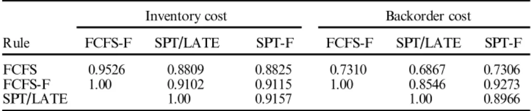
Our experimental results are consistent with the ® ndings of Lee (1987), Lee and Seah (1988), WemmerloÈv and Vakharia (1991), and Berkley (1993). In our experi-mental runs, the SPT/LATE rule performs signi® cantly better than the FCFS rule. Furthermore, the family-based scheduling rules can generate signi® cant improve-ments with respect to ¯ ow time and lateness-oriented performance measures over the FCFS rule as also shown by WemmerloÈv and Vakharia, since the ability to avoid setups is related to the performance of scheduling procedures in general. On the other hand, the SPT-F rule gives smaller inventory holding cost values than the FCFS-F rule, whereas the FCFS-F rule gives smaller backorder costs as expected. The relative success of the SPT/LATE rule can be attributed to the fact that it is a composite dispatching rule which combines the family and item-based methods. For the high setup time case, the performance of SPT/LATE is very similar to the SPT-F/ LATE since setup times dominate the individual kanban processing times in the updated processing time calculations, and all of the items from the same family will be scheduled consecutively. For the low setup time case, the SPT/LATE rule selects small withdrawal cycle lengths to minimize the backorder cost, and the LATE component of the rule, which is equivalent to the FCFS rule, is applied if any item is backlogged more than a predetermined number of periods. This fact can be observed in table 9, where we summarize the correlation coe cients using the two-tailed Pearson test between the dispatching rules for the inventory holding and backorder costs. In table 10, we present the actual results of each sequencing rule for the ® rst replication over 128 randomly generated runs. This table can provide the reader with a reference for selecting an operating policy in practice and also provide more information on the relative performance of the sequencing rules under varying con-ditions. In this table, we used an ` ’ to denote the best sequencing rule in each case. Furthermore, an ` ’ indicates the runs where the minimum cost and minimum T values were found by two di erent sequencing rules. For example, for the factor combination of…0101010†, the SPT/LATE rule found both the minimum cost and T
Inventory cost Backorder cost
Rule FCFS-F SPT/LATE SPT-F FCFS-F SPT/LATE SPT-F
FCFS 0.9526 0.8809 0.8825 0.7310 0.6867 0.7306
FCFS-F 1.00 0.9102 0.9115 1.00 0.8546 0.9273
SPT/LATE 1.00 0.9157 1.00 0.8966
Factors FCFS FCFS-F SPT/LATE SPT-F
A B C D E F G T Cost T Cost T Cost T Cost
0 0 0 0 0 0 0 2.00 600,050 *0.25 *59,470 0.25 297,893 2.00 600,050 0 0 0 0 0 0 1 4.00 996,456 *0.25 *88,427 0.25 573,378 4.00 996,456 0 0 0 0 0 1 0 2.00 600,050 0.50 93,458 *0.50 *77,709 0.50 103,309 0 0 0 0 0 1 1 4.00 996,456 0.50 132,611 *0.50 *90,248 0.50 132,513 0 0 0 0 1 0 0 *2.00 *600,050 *2.00 *600,050 4.00 635,912 *2.00 *600,050 0 0 0 0 1 0 1 *4.00 *996,456 *4.00 *996,456 *4.00 *996,456 *4.00 *996,456 0 0 0 0 1 1 0 *2.00 *600,050 *2.00 *600,050 4.00 635,912 *2.00 *600,050 0 0 0 0 1 1 1 *4.00 *996,456 *4.00 *996,456 *4.00 *996,456 *4.00 *996,456 0 0 0 1 0 0 0 2.00 1,089,819 0.50 207,247 *0.50 *148,769 0.50 230,879 0 0 0 1 0 0 1 4.00 1,828,645 0.50 327,607 *0.50 *194,360 0.50 335,590 0 0 0 1 0 1 0 1.00 318,223 1.00 199,106 *1.00 *197,880 1.00 199,103 0 0 0 1 0 1 1 1.00 442,954 1.00 199,421 *1.00 *199,023 1.00 199,418 0 0 0 1 1 0 0 2.00 1,089,819 2.00 1,089,819 *0.50 *707,040 2.00 1,089,819 0 0 0 1 1 0 1 4.00 1,828,645 4.00 1,828,645 *0.50 *1,072,965 4.00 1,828,645 0 0 0 1 1 1 0 4.00 1,198,141 1.00 1,121,254 *1.00 *635,623 1.00 660,793 0 0 0 1 1 1 1 4.00 1,862,885 4.00 1,862,885 *1.00 *1,088,776 1.00 1,142,900 0 0 1 0 0 0 0 0.50 484,038 *0.25 *59,470 0.25 297,893 0.50 484,038 0 0 1 0 0 0 1 2.00 846,895 *0.25 *88,427 0.25 573,378 2.00 846,895 0 0 1 0 0 1 0 0.50 482,474 0.50 93,458 *0.50 *77,709 0.50 103,309 0 0 1 0 0 1 1 2.00 846,895 0.50 132,611 *0.50 *90,248 0.50 132,513 0 0 1 0 1 0 0 *0.50 *484,037 *0.50 *484,037 2.00 551,520 *0.50 *484,037 0 0 1 0 1 0 1 *2.00 *846,895 *2.00 *846,895 4.00 869,706 *2.00 *846,895 0 0 1 0 1 1 0 0.50 480,137 *0.50 *479,661 2.00 551,520 0.50 479,665 0 0 1 0 1 1 1 *2.00 *846,895 *2.00 *846,895 4.00 869,706 *2.00 *846,895 0 0 1 1 0 0 0 0.50 159,566 0.50 331,720 *0.50 *147,229 0.50 230,879 0 0 1 1 0 0 1 0.50 181,246 0.50 561,078 *0.50 *147,354 0.50 335,590 0 0 1 1 0 1 0 1.00 318,223 0.50 159,869 0.50 150,494 *0.50 *150,383 0 0 1 1 0 1 1 1.00 442,954 1.00 199,421 0.50 172,189 *0.50 *171,958 0 0 1 1 1 0 0 2.00 930,897 2.00 930,897 *0.50 *347,255 0.50 903,302 0 0 1 1 1 0 1 2.00 1,506,827 2.00 1,506,827 *0.50 *477,953 2.00 1,506,827 0 0 1 1 1 1 0 1.00 955,331 1.00 544,120 *1.00 *297,523 1.00 313,805 0 0 1 1 1 1 1 2.00 1,684,696 2.00 1,684,828 4.00 1,702,654 *2.00 *1,684,392 0 1 0 0 0 0 0 1.00 739,241 0.25 113,787 0.25 93,153 *0.25 *92,065 0 1 0 0 0 0 1 2.00 1,360,614 0.25 160,612 0.25 109,297 *0.25 *106,228 0 1 0 0 0 1 0 1.00 739,241 0.50 171,801 *0.50 *112,406 0.50 113,399 0 1 0 0 0 1 1 2.00 1,360,614 0.50 275,869 0.50 150,977 *0.50 *149,987 0 1 0 0 1 0 0 1.00 739,241 1.00 739,241 *0.25 *320,929 0.25 554,388 0 1 0 0 1 0 1 2.00 1,360,614 2.00 1,360,614 *0.25 *467,968 0.25 1,046,538 0 1 0 0 1 1 0 2.00 753,580 2.00 753,580 0.50 341,992 *0.50 *324,828 0 1 0 0 1 1 1 2.00 1,360,614 2.00 1,360,614 0.50 584,045 *0.50 *580,665 0 1 0 1 0 0 0 2.00 1,845,140 0.50 510,023 *0.50 *338,734 0.50 380,726 0 1 0 1 0 0 1 4.00 3,353,777 0.50 922,634 *0.50 *563,493 0.50 648,289 0 1 0 1 0 1 0 2.00 1,845,140 1.00 824,377 1.00 *594,051 *0.50 793,115 ** 0 1 0 1 0 1 1 4.00 3,353,777 1.00 1,524,823 1.00 *1,051,924 *0.50 1,469,819 ** 0 1 0 1 1 0 0 4.00 2,240,146 2.00 2,027,954 *0.50 *1,669,132 2.00 1,986,441 0 1 0 1 1 0 1 4.00 3,562,777 4.00 3,562,777 *0.50 *2,459,189 2.00 3,530,211 0 1 0 1 1 1 0 4.00 2,322,191 4.00 2,230,380 *1.00 *1,946,901 4.00 2,216,977 0 1 0 1 1 1 1 4.00 3,799,962 4.00 3,591,764 *4.00 *3,553,504 *4.00 *3,553,504 0 1 1 0 0 0 0 0.25 99,992 0.25 91,351 *0.25 *88,369 0.25 91,410 0 1 1 0 0 0 1 0.25 110,653 0.25 91,376 *0.25 *88,402 0.25 91,435 0 1 1 0 0 1 0 0.50 134,849 0.50 101,608 *0.50 *83,039 0.50 101,371 0 1 1 0 0 1 1 0.50 195,068 0.50 121,117 *0.50 *83,039 0.50 114,452 0 1 1 0 1 0 0 2.00 716,696 2.00 716,696 *0.25 *97,608 0.25 135,486 0 1 1 0 1 0 1 2.00 1,239,154 2.00 1,239,154 *0.25 *125,457 0.25 200,194 0 1 1 0 1 1 0 2.00 716,696 2.00 716,696 0.50 252,145 *0.50 *217,461 0 1 1 0 1 1 1 2.00 1,239,154 2.00 1,239,154 0.50 432,263 *0.50 *361,269 0 1 1 1 0 0 0 1.00 1,189,601 0.50 314,690 0.50 233,173 *0.50 *216,192 0 1 1 1 0 0 1 1.00 2,246,923 0.50 529,411 0.50 346,933 *0.50 *307,146 0 1 1 1 0 1 0 2.00 1,717,251 1.00 622,729 1.00 *484,067 *0.50 608,804 ** 0 1 1 1 0 1 1 4.00 2,989,783 1.00 1,129,149 1.00 *820,729 *0.50 1,103,077 ** 0 1 1 1 1 0 0 2.00 1,865,432 2.00 1,865,415 *0.50 *1,332,839 2.00 1,865,547 0 1 1 1 1 0 1 4.00 3,178,119 4.00 3,178,119 *0.50 *1,858,485 4.00 3,178,119 0 1 1 1 1 1 0 4.00 2,087,688 2.00 1,989,334 *1.00 *1,527,532 2.00 1,854,698 0 1 1 1 1 1 1 4.00 2,948,405 4.00 2,948,249 *1.00 *2,090,650 4.00 2,948,672
Factors FCFS FCFS-F SPT/LATE SPT-F
A B C D E F G T Cost T Cost T Cost T Cost
1 0 0 0 0 0 0 2.00 1,070,045 0.50 162,671 0.50 176,590 *0.50 *156,914 1 0 0 0 0 0 1 2.00 1,896,176 0.50 236,039 0.50 247,618 *0.50 *216,355 1 0 0 0 0 1 0 1.00 789,404 1.00 *211,876 *0.50 241,532 1.00 219,495 ** 1 0 0 0 0 1 1 1.00 1,420,300 1.00 255,067 *0.50 390,354 1.00 *253,312 ** 1 0 0 0 1 0 0 2.00 1,070,045 2.00 1,078,057 0.50 893,310 *0.50 *766,463 1 0 0 0 1 0 1 2.00 1,896,176 2.00 1,906,835 *0.50 *1,304,168 0.50 1,451,500 1 0 0 0 1 1 0 2.00 1,204,315 1.00 592,447 1.00 580,968 *1.00 *580,059 1 0 0 0 1 1 1 4.00 1,938,634 1.00 1,040,885 1.00 1,002,274 *1.00 *995,338 1 0 0 1 0 0 0 2.00 2,086,140 1.00 714,588 *1.00 *477,884 1.00 486,371 1 0 0 1 0 0 1 4.00 3,730,477 1.00 1,204,210 *1.00 *719,693 1.00 733,857 1 0 0 1 0 1 0 4.00 2,293,080 2.00 961,875 2.00 870,796 *2.00 *756,665 1 0 0 1 0 1 1 4.00 3,777,937 2.00 1,571,477 2.00 1,434,227 *2.00 *1,157,985 1 0 0 1 1 0 0 4.00 2,544,535 2.00 2,358,068 *1.00 *1,914,514 1.00 2,093,618 1 0 0 1 1 0 1 4.00 3,898,358 4.00 3,780,467 *1.00 *3,187,300 4.00 3,778,285 1 0 0 1 1 1 0 4.00 2,783,713 2.00 2,486,817 2.00 2,119,621 *2.00 *2,059,809 1 0 0 1 1 1 1 4.00 4,159,214 4.00 3,756,212 2.00 3,618,560 *2.00 *3,500,121 1 0 1 0 0 0 0 0.50 891,929 *0.50 *143,793 0.50 184,694 0.50 175,663 1 0 1 0 0 0 1 2.00 1,537,759 *0.50 *153,642 0.50 265,820 0.50 244,043 1 0 1 0 0 1 0 1.00 638,717 0.50 143,135 *0.50 *122,927 0.50 126,917 1 0 1 0 0 1 1 1.00 1,083,269 0.50 181,772 *0.50 *131,823 0.50 134,711 1 0 1 0 1 0 0 2.00 925,036 *0.50 *228,514 2.00 980,479 0.50 269,884 1 0 1 0 1 0 1 2.00 1,537,759 *0.50 *353,980 4.00 1,588,807 0.50 422,648 1 0 1 0 1 1 0 2.00 951,624 1.00 571,509 0.50 414,876 *0.50 *286,069 1 0 1 0 1 1 1 2.00 1,563,655 1.00 952,919 0.50 665,769 *0.50 *454,210 1 0 1 1 0 0 0 1.00 1,516,065 1.00 381,746 0.50 289,909 *0.50 *279,392 1 0 1 1 0 0 1 1.00 2,695,425 1.00 475,156 0.50 403,945 *0.50 *381,208 1 0 1 1 0 1 0 2.00 1,357,571 2.00 623,962 1.00 *494,474 *0.50 526,402 ** 1 0 1 1 0 1 1 2.00 2,427,942 2.00 855,547 *1.00 *657,777 2.00 726,748 1 0 1 1 1 0 0 2.00 1,944,679 1.00 1,776,734 *0.50 *1,156,988 0.50 1,231,747 1 0 1 1 1 0 1 2.00 3,086,255 2.00 3,038,048 *0.50 *1,812,598 1.00 2,098,559 1 0 1 1 1 1 0 4.00 2,548,944 2.00 1,393,079 *1.00 *1,286,621 2.00 1,377,621 1 0 1 1 1 1 1 4.00 3,306,245 2.00 2,048,832 *1.00 *1,836,494 2.00 1,940,540 1 1 0 0 0 0 0 1.00 1,651,314 1.00 407,364 *0.50 *261,147 0.50 262,099 1 1 0 0 0 0 1 1.00 3,183,720 1.00 696,314 0.50 425,411 *0.50 *424,131 1 1 0 0 0 1 0 2.00 1,540,750 2.00 615,826 *1.00 *442,063 1.00 458,974 1 1 0 0 0 1 1 2.00 2,893,019 2.00 990,494 *1.00 *769,427 1.00 802,751 1 1 0 0 1 0 0 4.00 2,240,562 2.00 2,018,904 *0.50 *1,373,749 2.00 2,118,712 1 1 0 0 1 0 1 4.00 3,733,484 4.00 3,563,901 *0.50 *2,230,343 4.00 3,696,462 1 1 0 0 1 1 0 4.00 2,302,477 4.00 2,246,437 *0.50 *1,672,977 2.00 2,135,739 1 1 0 0 1 1 1 4.00 3,837,775 4.00 3,700,784 *0.50 *2,559,757 4.00 3,656,344 1 1 0 1 0 0 0 4.00 4,390,898 4.00 3,319,699 4.00 *3,170,542 *2.00 3,427,358 ** 1 1 0 1 0 0 1 4.00 6,854,481 4.00 4,553,177 4.00 *4,182,788 *2.00 5,794,732 ** 1 1 0 1 0 1 0 4.00 5,382,560 4.00 4,598,943 4.00 *4,000,059 *2.00 4,137,725 ** 1 1 0 1 0 1 1 4.00 8,365,626 4.00 6,458,210 *4.00 *5,436,028 4.00 6,330,285 1 1 0 1 1 0 0 4.00 5,903,208 4.00 5,835,746 4.00 *5,614,082 *2.00 6,101,923 ** 1 1 0 1 1 0 1 4.00 8,498,082 4.00 8,213,472 *4.00 *7,675,072 4.00 9,455,052 1 1 0 1 1 1 0 4.00 7,397,175 4.00 6,885,947 *2.00 *6,383,950 2.00 6,735,029 1 1 0 1 1 1 1 4.00 10,353,970 4.00 9,228,932 *4.00 *8,696,289 4.00 10,365,629 1 1 1 0 0 0 0 1.00 1,503,533 0.50 256,052 0.50 184,694 *0.50 *173,133 1 1 1 0 0 0 1 1.00 2,874,186 0.50 411,307 0.50 265,820 *0.50 *237,928 1 1 1 0 0 1 0 2.00 1,513,135 1.00 524,155 *1.00 *351,874 1.00 363,758 1 1 1 0 0 1 1 2.00 2,744,448 1.00 921,070 *1.00 *588,527 1.00 604,057 1 1 1 0 1 0 0 2.00 1,803,901 2.00 1,746,031 *0.50 *1,121,252 2.00 1,820,493 1 1 1 0 1 0 1 4.00 3,153,207 2.00 3,079,366 *0.50 *1,821,384 4.00 3,175,458 1 1 1 0 1 1 0 4.00 2,070,514 2.00 1,907,054 *0.50 *1,376,428 2.00 1,824,037 1 1 1 0 1 1 1 4.00 3,330,396 4.00 3,220,930 *0.50 *2,138,776 4.00 3,219,481 1 1 1 1 0 0 0 2.00 3,466,929 4.00 2,126,993 *2.00 *1,678,878 2.00 2,153,014 1 1 1 1 0 0 1 4.00 5,167,284 4.00 2,447,540 *2.00 *2,389,044 2.00 3,352,615 1 1 1 1 0 1 0 4.00 4,047,221 4.00 2,815,685 *2.00 *2,585,073 2.00 2,621,054 1 1 1 1 0 1 1 4.00 5,944,762 4.00 3,245,821 *4.00 *3,006,017 4.00 3,509,381 1 1 1 1 1 0 0 4.00 4,791,975 4.00 *4,315,901 *2.00 4,365,649 2.00 4,885,361 ** 1 1 1 1 1 0 1 4.00 6,604,624 *4.00 *5,647,182 4.00 6,266,995 4.00 6,922,630 1 1 1 1 1 1 0 4.00 5,823,073 4.00 5,186,707 *2.00 *4,968,744 2.00 5,195,590 1 1 1 1 1 1 1 4.00 7,575,943 4.00 6,345,376 *4.00 *6,145,755 4.00 7,112,599
values. For…0101010†, the SPT/LATE rule found the minimum cost value, whereas the SPT-F gave the minimum T value.
For each sequencing rule, we also applied a two-way analysis of variance (ANOVA) test on the performance measures of inventory holding and backorder costs. All of the factors were statistically signi® cant for the inventory holding cost with p40:000. For the backorder cost, all of the factors except the S/P ratio for all
rules and the imbalance for the FCFS rule were signi® cant with p40:000. Of these
factors A, B and C directly a ect the product variety and the amount to be pro-duced, hence the inventory holding and backorders costs. When we analyse the systems with imbalance, although we allocate di erent numbers of kanbans to each stage to increase ¯ exibility, the performance of the kanban system declines with an imbalance in the system. The FCFS rule is not statistically a ected since it maintains consistent kanban priorities from stage to stage and prevents kanban passing. This result is consistent with the ® ndings of Huang et al. (1983) and Gupta and Gupta (1989). Gupta and Gupta (1989) show that in order to achieve the highest e ciency, all the stages of the kanban system should be balanced. Huang et al. (1983) show that if bottlenecks occur regularly, the system performance declines. They conclude that additional kanbans at each stage are no help at all when there is a bottleneck in the system. When we analyse the systems with low and high S/P ratios we see that when S/P ratio increases, the maximum inventory levels and inventory holding costs increase, and ® ll rates decrease. That is to say, system per-formance declines when setup times become considerable. This ® nding is consistent with the study of Mittal and Wang (1992). In a simulation study the authors show that after a threshold value for the setup times, the number of kanbans required for smooth ¯ ow tends towards in® nite. Finally, the signi® cance of factor D, demand variability, depends on the fact that items with large demand ¯ uctuations in¯ ate actual lead times and decrease the ® ll rates.
4. Conclusions
In this study, we give an overview of the literature on kanban systems in two parts. In the ® rst part, the models on determining the design parameters are explained by using a tabular format to compare di erent models. In the second part, we present the models for sequencing the production kanbans at each stage in order to investigate the interactions between the design and operational issues. Based on the literature reviewed in this paper, the limitations of the existing studies can be summarized as follows:
. Very few studies exist that consider the kanban sizes explicitly, i.e. Gupta and
Gupta (1989), Karmarkar and Kekre (1989), Philipoom et al. (1996), Moeeni et al. (1997). In fact, the number of kanbans required depends on kanban sizes and these parameters together a ect the system performance. Therefore these parameters should be determined simultaneously, not sequentially.
. The existing JIT production planning models deal mainly with smoothing
production schedules. None of the studies consider the impact of operational issues on the design parameters. Since the ® nal assembly schedule determines production orders for all of the preceding stages, it is commonly assumed that this schedule can be propagated back through system using the FCFS rule. Therefore, the scheduling in kanban systems needs more elaboration,
espe-cially under the di erent experimental conditions where the demands may be variable, setup times may be high, and the system may be imbalanced.
. Even though dual-card kanban systems are periodic in nature, there are a
limited number of studies on periodic review systems. The typical assumption is that kanban withdrawal mechanism is instantaneous. We showed that the most commonly used combination of the FCFS rule with the instantaneous kanban withdrawal mechanism may not be a good policy for all experimental conditions. In contrary, the FCFS rule performs better when the withdrawal cycle lengths are long enough to justify the setup times.
We also analysed the impact of operational issues, such as kanban sequences and actual lead times, on the design parameters of the withdrawal cycle length, kanban size and number of kanbans using the four commonly used sequencing rules in the literature. We observed that the withdrawal cycle lengths are not robust to sched-uling decisions such that item-based methods prefer longer withdrawal cycle lengths whereas the family-based rules prefer shorter ones. One of the main assumptions of JIT is repetitive manufacturing. Therefore, factors that adversely a ect the repetitive nature of the system, i.e. increasing the product variety and decreasing product standardization, reduce the performance of kanban systems. It is observed analyti-cally that perfectly balanced lines outperform the imbalanced ones even when we vary the number of kanbans at each stage. The factors that a ect the congestion of the system, such as demand mean and variability, number of families, and number of parts in each family, also a ect system performance. The item-based rules perform better than the family-based rules in terms of backorder cost and ® ll rates if the system load is loose, and the opposite is true as the system load increases. When setup times become considerable system performance declines, since large setup times require large lot sizes, and large lot sizes in¯ ate lead times and in-process inventory levels. For high setup time cases algorithms that can decrease the total setup time perform better than the others, i.e. family-based rules outperform item-based rules. In general, the family-item-based rules are more robust against increases in setup time. Finally, more sophisticated scheduling algorithms should be developed to determine kanban sequences in order to increase the e ectiveness of these systems. References
Akturk, M. S. andBalkose, H. O.,1996, Part-machine grouping using a multi-objective cluster analysis. International Journal of Production Research,34, 2299± 2315.
Askin, R. G., Mitwasi, M. G. and Goldberg, J. B.,1993, Determining the number of kanbans in multi-item just-in-time systems.IIE Transactions,25, 89± 97.
Bard, J. F.andGolony, B.,1991, Determining the number of kanbans in a multiproduct, multistage production system. International Journal of Production Research, 29, 881±
895.
Berkley, B. J., 1992, A review of the kanban production control research literature.
Production and Operations Management,1,393± 411.
Berkley, B. J.,1993, Simulation tests of FCFS and SPT sequencing in kanban systems.
Decision Sciences,24, 218± 227.
Berkley, B. J., 1996, A simulation study of container size in two-card kanban system.
International Journal of Production Research, 34, 3417± 3445.
Berkley, B. J.andKiran, A. S.,1991, A simulation study of sequencing rules in a kanban-controlled ¯ ow shop.Decision Sciences,22, 559± 582.
Bitran, G. R.andChang, L.,1987, A mathematical programming approach to a determi-nistic kanban system. Management Science, 33, 427± 441.
Groenevelt,H.,1993, The just-in-time system. In: Handbooks in OR & MS volume 4, edited by S. C. Graves, A. H. G. Rinnooy Kan, and P. H. Zipkin (Amsterdam: Elsevier), pp. 629± 670.
Gupta,Y.P.andGupta,M.C.,1989, A system dynamics model for a multi-stage, multi-line dual-card JIT-kanban system. International Journal of Production Research, 27, 309±
352.
Huang, C. C.andKusiak, A.,1996, Overview of kanban systems.International Journal of
Computer Integrated Manufacturing,9, 169± 189.
Huang, P. Y., Rees, P. L.andTaylor, B. W.III, 1983, Simulation analysis of the Japanese just-in-time technique (with kanbans) for a multiline, multistage production system.
Decision Sciences,14, 326± 344.
Karmarkar, U.,1993, Manufacturing lead times, order release and capacity loading. In:
Handbooks in OR & MS volume 4, edited by S. C. Graves, A. H. G. Rinnooy Kan,
and P. H. Zipkin (Amsterdam: Elsevier), pp. 287± 329.
Karmarkar, U. and Kekre, S., 1989, Batching policy in kanban systems. Journal of
Manufacturing Systems,8,317± 328.
Kimura, O.andTerada, H.,1981, Design and analysis of pull system: a method of multi-stage production control.International Journal of Production Research,19, 241± 253.
Lee, L. C.,1987, Parametric appraisal of the JIT system. International Journal of Production
Research,25, 1415± 1429.
Lee,L. C.andSeah, K.H. W.,1988, JIT and the e ects of varying process and set-up times.
International Journal of Operations and Production Management,6,186± 190.
Li, A.and Co, H. C.,1991, A dynamic programming model for the kanban assignment problem in a multistage multiperiod production system. International Journal of
Production Research,29, 1± 16.
Lummus, R. R.,1995, A simulation analysis of sequencing alternatives for JIT lines using kanbans. Journal of Operations Management, 13, 183± 191.
Mitra, D.andMitrani, I.,1990, Analysis of a kanban discipline for cell coordination in production lines. I.Management Science,36, 1548± 1566.
Mittal, S.andWang, H. P.,1992, Simulation of JIT production to determine number of kanbans. International Journal of Advanced Manufacturing Technology,7,292± 305.
Mitwasi, M. G.andAskin, R. G.,1994, Production planning for a multi-item, multi-stage kanban system.International Journal of Production Research,32, 1173± 1195.
Miyazaki, S., Ohta, H.andNishiyama, N.,1988, The optimal operation planning of kan-ban to minimize the total operation cost.International Journal of Production Research,
26, 1605± 1611.
Monden, Y.,1984, A simulation analysis of the Japanese just-in-time technique (with kan-bans) for a multiline, multistage production system: a comment.Decision Sciences,15, 445± 447.
Monden, Y.,1993, Toyota Production System second edition, (Norcross, GA: Engineering and Management Press).
Moeeni, F., Sanchez, S. M.andVakharia, A. J.,1997, A robust design methodology for Kanban system design.International Journal of Production Research, 35, 2821± 2838.
Ohno,K.,Nakashima,K.andKojima,M.,1995, Optimal numbers of two kinds of kanbans in a JIT production system. International Journal of Production Research, 33, 1387±
1401.
Philipoom, P. R., Rees, L. P.andTaylor, B. W.III, 1996, Simultaneously determining the number of kanbans, container sizes, and the ® nal-assembly sequence of products in a just-in-time shop.International Journal of Production Research,34, 51± 69.
Philipoom, P. R., Rees, L. P., Taylor, B. W. III, and Huang, P. Y.,1990, A mathematical programming approach for determining workcentre lotsizes in a just-in-time system with signal kanbans.International Journal of Production Research,28, 1± 15.
Ragatz,G.L.andMabert,V.A.,1984, A simulation analysis of due date assignment rules.
Journal of Operations Management,5,27± 39.
Rees, L. P., Philipoom, P. R., Taylor, B. W. III, and Huang, P. Y.,1987, Dynamically adjusting the number of kanbans in a just-in-time production system using estimated values of leadtime. IIE Transactions,19, 199± 207.
Savsar,M.,1996, E ects of kanban withdrawal policies and other factors on the performance of JIT systemsÐ a simulation study. International Journal of Production Research,34, 2879± 2899.
Takahashi, K.,1994, Determining the number of kanbans for unbalanced serial production systems. Computers and Industrial Engineering,27, 213± 216.
Wang, H.andWang, H.P.,1990, Determining the number of kanbans: A step toward non-stock-production. International Journal of Production Research,28, 2101± 2115.
Wemmerlov, U.andVakharia, A. J.,1991, Job and family scheduling of a ¯ ow-line manu-facturing cell: a simulation study. IEE Transactions, 23, 383± 394.