A 3D dynamic model of a spherical wheeled self-balancing robot

A 3D Dynamic Model of a Spherical Wheeled Self-Balancing Robot

Ali Nail Inal

, ¨

Omer Morg¨ul

and Uluc. Saranlı

Abstract— Mobility through balancing on spherical wheels

has recently received some attention in the robotics literature. Unlike traditional wheeled platforms, the operation of such platforms depends heavily on understanding and working with system dynamics, which have so far been approximated with simple planar models and their decoupled extension to three dimensions. Unfortunately, such models cannot capture inherently spatial aspects of motion such as yaw motion arising from the wheel rolling motion or coupled inertial effects for fast maneuvers. In this paper, we describe a novel, fully-coupled 3D model for such spherical wheeled platforms and show that it not only captures relevant spatial aspects of motion, but also provides a basis for controllers better informed by system dynamics. We focus our evaluations to simulations with this model and use circular paths to reveal advantages of this model in dynamically rich situations.

I. INTRODUCTION

Robust, efficient and controllable land-based mobility is one of the important but difficult challenges faced by the robotics community. Morphologically, there are many op-tions that can be considered including wheeled [1], tracked [2], legged [3, 4] and even leaping [5] designs, some inspired from examples in biology and others based on purely en-gineered solutions. A recent addition to these alternatives has been through robot platforms that actively balance on “spherical wheels” [6, 7], also known as Ballbot platforms. Such robots potentially combine advantages of wheeled systems through their continuous contact with the ground with desirable features of bipedal morphologies for their compatibility with environments designed for human use. However, their complexity is far greater than that of wheeled systems since their operation is inherently dynamic and cannot be controlled through simpler kinematic methods.

Despite the simplicity of the principle behind this mor-phology, partially shared by planar balancing systems such as the Segway and others, the omnidirectional mobility it affords is impressive. However, starting from the first experimental instantiations of this idea that were based on an inverse mouse ball design [6, 8] to later versions that used omnidirectional wheel contact with the sphere for better control affordance and reduced friction [7, 9], accurate control of Ballbot dynamics for fast maneuvers remains to be a challenging problem. Initial inquiries focused on motion along linear paths, which can be reduced to a 2D model in the saggital plane, using PI control on the ball velocity and an LQR controller design as an outer loop around the linearized 1_{A. N. Inal and O. Morg¨ul are with the Dept. of} Electrical Engineering, Bilkent University, Ankara, Turkey

{inal,morgul}@ee.bilkent.edu.tr

2_{U. Saranlı is with the Dept. of Computer Engineering, Middle East} Tech-nical University, Ankara, Turkeysaranli@ceng.metu.edu.tr

system to control body attitude [6, 8]. As far as mathematical models are concerned, it has not been possible to go too far beyond this planar approximation, with spatial extensions relying on a decoupled combination of two planar models in two orthogonal directions of the horizontal plane. Recent extensions include more sophisticated control methods for both the stabilization of body attitude degrees of freedom as well as the design of optimal attitude trajectories to travel along desired robot paths [10, 11]. Inertial disturbances and loads on the robot body reveal further limitations associated with decoupled models and their inability to deal with dynamic situations [12]. Even though recent work extends on these behavioral primitives used as a basis for more complex trajectories through planning [13], there has not been much progress in the accuracy and expressivity of underlying mathematical models.

Unfortunately, highly dynamic and fast maneuvers that are most likely to distinguish the capabilities of the Ball-bot platform from more traditional modes of mobility are precisely those for which decoupled planar models, which we call 2.5D models in this paper, lose their accuracy. Maneuvers with large accelerations require body orientations that deviate substantially from the vertical, creating both significant yaw rotation as well as coupled inertial effects. In light of these limitations, there is a clear need for more realistic mathematical models for Ballbot systems capable of supporting more challenging dynamic behaviors.

In this paper, we introduce a novel, three-dimensional model for Ballbot platforms that can capture aspects of its motion that are beyond the capabilities of 2.5D models. We first derive the equations of motion for our model, which are then used as a basis for both a simulation model for the platform, as well as novel inverse-dynamics controllers for accurate control of body attitude. We then illustrate the performance of these model-based controllers for tracking circular body attitude trajectories. We also present simulation results to establish that the new model recovers the ability to model natural yaw dynamics arising from the rolling con-straint between the ground and the ball, impossible to capture with 2.5D models. Finally, we provide a characterization of how different circular trajectories in the body attitude space can be used to follow circular paths with the robot, illustrating the potential utility of the 3D model for motion planning and execution with Ballbot platforms.

II. BALLBOTDYNAMICS ANDCONTROL

A. The Planar Ballbot Model

Many initial attempts towards the analysis and control of the Ballbot platform relied on a two dimensional model of 2012 IEEE/RSJ International Conference on

Intelligent Robots and Systems

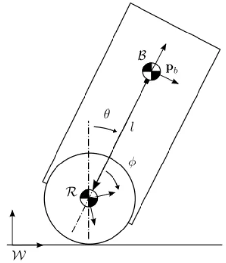
B R W pb l θ φ

Fig. 1. The 2D Ballbot model on the saggital plane

the platform constrained to the saggital plane [6, 8]. This planar model, illustrated in Figure 1, consists of a rigid robot body connected to the center of a rolling ball through an actuated pin joint at a distancel from the body center of mass (COM). Conveniently, the rolling contact constraint for this model can be expressed as a holonomic constraint between the horizontal position and the angle of the ball, making it possible to use an Euler-Lagrange approach to derive the equations of motion. Details of these derivations are easily found in the existing literature on the Ballbot platform and will be omitted in this paper for space considerations. B. Decoupled 2.5D Ballbot Model

The main difference of the Ballbot platform from planar balancing systems such as the Segway or other similar systems is its ability to freely move in all directions on the horizontal plane. A 2D model on the saggital plane would not be sufficient to capture all of its distinguishing capabilities. For this reason, most existing literature on the analysis and control of this platform adopts a “2.5D” model wherein two decoupled 2D models in two orthogonal saggital planes in the ambient space are assumed to accurately represent the motions of the 3D platform. However, this approach has a number of problems that effect its accuracy and utility for dynamic maneuvers with the Ballbot platform:

1) The use of such a 2.5D model is incapable of modeling natural yaw dynamics for the Ballbot. This becomes particularly relevant when the upright Ballbot posture needs to be abandoned towards fast and dynamic maneuvers. Since such maneuvers are among the most interesting potential capabilities of this morphology, the 2.5D model is likely to be limiting and insufficient in the long run.

2) Without the ability to model any yaw dynamics, the 2.5D model cannot predict the orientation of the actua-tion mechanism with respect to the ball, or the ball with respect to the ground. This makes it difficult to model interactions between these components, which were found to be important components in understanding

Ballbot behavior. A mathematical model that is capable of easily and naturally incorporating their effects would have substantial utility in the design of sufficiently accurate behavioral controllers.

3) Any extensions of the system, such as the addition of arms [12], or asymmetric loads, would make the 2.5D model even less accurate. Consequently, a fully coupled 3D model is necessary if accurate behavioral control is desired with such external loads and inertial changes in the robot structure.

These observations constitute the basis of our motivation towards the construction of a coupled, 3D model for the Ball-bot that can accurately capture all aspects of its dynamics. C. The Fully Coupled 3D Ballbot Model

B R W (pb, qb) (pr, qr) pc l ac

Fig. 2. The fully coupled 3D Ballbot model

1) Basic Structure and Parameters: Our new 3D Ballbot model is shown in Figure 2 and consists of a rigid body with massmb and inertia matrix Ib “attached” to the center of a

spherical ball with radius rr, mass mr and inertia matrix

Ir through a spherical joint actuated with torque vector τ .

Three coordinate frames are defined: an inertial world frame W, a “ball frame” R located at the center of the rolling ball and a “body frame”B located at the COM of the robot body. Based on the inverse mouse-ball drive Ballbot design of [11], we assume that only two components of the actuation torque τ in B are directly controlled, and the Z component τbz is a

constraint torque to eliminate relative yaw rotation between the body and the ball. We assume that ground frictional forces and the vertical torqueτrzon the ball prevent it from

slipping horizontally and in the yaw direction, implementing a pure rolling constraint. Viscous damping on the ball is implemented through separate horizontal torques on the ball. The distance betweenR and B remains fixed at l. Assum-ing that thez axis of B is aligned with the line acconnecting

the COMs of the ball and the body, the ball COM in B is a constant vector [0, 0, −l]T

orientations of the body and the ball in W are denoted with (pb, qb) and (pr, qr), respectively. The contact point

between the ball and the ground is denoted with pc.

2) Free-Body Analysis and Constraints: As noted above, Ballbot has a no-slip constraint between the ball and the ground. This reduces to a holonomic constraint for the planar model, but remains as a nonholonomic constraint on the ball angular velocity for the 3D model. Consequently, we will find it convenient to formulate the dynamics through a free-body analysis, which will also yield various constraint forces between different components in the system.

We first define the unconstrained state of the system as a combination of system poses and momenta to yield

x:= [pb, Pb, qb, Lb, pr, Pr, qr, Lr]T , (1)

where all coordinates are with respect toW unless otherwise indicated and P and L denote linear and angular momenta, respectively. The equations of motion can be formulated by finding unknown accelerations and constraint forces, which we collect in an unknown vector as

U:= [ ˙Pb, ˙Lb, ˙Pr, ˙Lr, Fb, Fr, τbz, τrz]T , (2)

where Fband Frare constraint forces applied by the ball to

the body, and the ground to the ball, respectively. Ballbot dynamics involve four different constraints: 1) The ball COM and the ball joint must coincide, with

qb⋆ [0, 0, −l]T ⋆ q∗b+ pb = pr (3)

where ⋆ denotes quaternion multiplication and q∗ b is

the quaternion conjugate of qb.

2) The ball has pure rolling motion, with

Pr= mr[0, 0, −rr]T × (I−1_r,WLr) (4)

where Ir,W := R(qb)IrR(qb)T is the ball inertia in

W and R(qb) is the body rotation matrix.

3) The ball has no yaw motion inW, with h [0, 0, 1], (I−1

r,WLr) i = 0 , (5)

where h·, ·i denotes the vector inner product.

4) The body has no yaw motion relative to the ball, with h [0, 0, 1], (RT_(q

b)(I−1_b,WLb− I−1_r,WLr)) i = 0 . (6)

The equations of motion derived in the next section will incorporate these constraints into the solution of unknown system accelerations and forces.

3) Equations of Motion: The first six equations are ob-tained from Newton’s law on linear accelerations as

˙

Pi= Fi+ [0, 0, −mig]T , (7)

where i = r for the ball and i = b for the body. Similarly, another six equations corespond to rotational accelerations

˙Lb = (qb⋆ [0, 0, −l]T⋆ qb∗) × Fb+ qb⋆ τ ⋆ q∗b (8)

˙Lr = [0, 0, −rr]T × Fr− qb⋆ τ ⋆ q∗b+ τf . (9)

where τf denotes the viscuous frictional torque acting on

the ball proportional to its angular velocity. The ball joint

constraint of (3) yields three more equations through its second derivative and the final five equations result from first derivatives of the constraints (4), (5) and (6) on system velocities. These relations yield a system of 20 equations with the 20 unknowns in U expressed in matrix form as

MU= N , (10)

which can be solved to yield the unknown accelerations and forces as U = M−1_{N, assuming that the matrix M is}

invertible, which is always the case for mechanical systems of this kind unless problematic model components such as Coulomb friction are considered. We leave the details of these derivations out for space considerations, noting that matrix forms for quaternion multiplication and cross product operations allow substantial simplifications and the resulting equations are all linear in the unknown quantities of U.

Once the unknown accelerations and forces are found, the equations of motion take the form

˙x = f (x, τbx, τby) , (11)

where the derivatives of configuration variables are provided by kinematic relations as

˙pi = Pi/mi (12)

˙qi = (I−1i,WLi) ⋆ qi/2 , (13)

where, once again,i = r for the ball and i = b for the body. D. Attitude Control through Inverse Dynamics

Independent of the nonholonomic contact constraints be-tween the ball and the ground, Ballbot dynamics are under-actuated for its motion inW. Consequently, the position and orientation of the ball (external variables) cannot be directly controlled through available control inputs. Control of the Ballbot motion must regulate and use body attitude states (shape variables) to modulate ball dynamics towards desired behavior. A detailed account of the reasons and consequences of these properties can be found in [13, 14].

In light of this limitation, accurate realization of desired shape variable trajectories becomes critically important if specific motions on external variables are to be realized. In previous work, this was accomplished through PID control [13], which is prone to tracking errors particularly when the body pose deviates substantially from its vertical posture and inertial effects become significant at high speeds. One of our contributions in this paper is the design of an inverse-dynamics controller based on our 3D model for controlling Ballbot’s body attitude.

In this section, we describe how our 3D model can be used as a basis for computed torque control, cancelling gravitational and inertial effects on the body attitude to yield accurate attitude control for the Ballbot. We use this controller in subsequent sections to illustrate various features of the 3D model with respect to its ability to capture interesting behaviors on external variables.

The primary goal of our inverse dynamics controller is to first cancel out accelerations on body attitude degrees

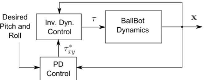
BallBot Dynamics Inv. Dyn. Control PD Control Desired Pitch and Roll x τ_xy∗ τ

Fig. 3. Block diagram for Inverse Dynamics and PD Controllers acting on the Ballbot plant.

of freedom due to the Ballbot dynamics, then use a PD controller to stabilize them around desired trajectories that might be generated, for example, by an optimal planner as described in [13]. Figure 3 illustrates the structure of this control strategy. PD Gains Desired Pitch Desired Roll Body Roll + − + − Body Pitch τ_xy∗

Fig. 4. Detailed block diagram for PD controller to stabilize the attitude dynamics within the inverse dynamics controller.

In order to accomplish this goal, we first augment the previously defined vector of unknowns of (2) with the control inputs to be solved, yielding

U′_{:= [ ˙P}

b, ˙Lb, ˙Pr, ˙Lr, Fb, Fr, τbz, τrz, τbx, τby]T . (14)

We then introduce two new constraints to reduce attitude dynamics to only experience the PD controller with

h[1, 0, 0], ˙Lbi = τx∗ (15)

h[0, 1, 0], ˙Lbi = τy∗ (16)

where τ∗

x andτy∗ are the stabilizing PD torques inW

com-puted as shown in Figure 4. The solution to the augmented constraint equation U′ _{= (M}′₎−1_N′ _{yields control torques}

that effectively cancel out any dynamics on body attitude coordinates, only leaving decoupled stabilizing torques in place.

III. SIMULATIONSTUDIES ANDDISCUSSION

A. Simulation Environment

Our simulation studies of subsequent sections are based on numerical integration of the equations of motion (11), solving for the vector of unknown accelerations and forces through (10) for each evaluation. We use Matlab’s ode45 integrator with a relative tolerance of10−3 _{and a maximum}

time step of 10−1_{s. In order to ensure that the constraints}

defined by (3), (4), (5) and (6) do not drift in time due to numerical integration errors, we peridocially reset the system state to the closest state that satisfies the constraints once every 1s. Consequently, constraint errors always stay

below10−6_{in magnitude our simulations. In the absence of}

these corrections, constraint drift becomes problematic for simulations of duration larger than100s.

−10 0 10 −10 −5 0 5 10 θ x (deg) θy (deg) −1 0 1 −1 −0.5 0 0.5 1 x (m) y (m) Spiral start Circle start Path end

Fig. 5. An example simulation with the 3D Ballbot model, starting from an upright posture and sprialing out to a circular attitude trajectory. Left: Body attitude trajectory, Right: Ball trajectory in W. This example has an attitude reference with period tcycle= 5s and amplitude Amax= 10deg. θxand θyare attitude angles around the x and y axes, respectively.

Subsequent sections on our simulation results exclusively consider periodic, circular trajectories in body attitude co-ordinates (with periodtcycle and amplitudeAmax),

hypoth-esized to yield similarly circular paths for the ball COM. Unlike linear paths, such circular trajectories exercise dy-namically dexterous capabilities of the platform. To ensure smooth transients and to prevent falling, we begin our simulations at t = 0 from an upright body posture with qb = [1, 0, 0, 0]T. We then command the body attitude to

follow a pattern spiraling out for a duration of tsetup to

react its periodic, circular pattern until at = tf inal chosen

to be sufficiently large to ensure convergence to steady-state. An example of this attitude profile and the resulting robot motion in W is illustrated in Figure 5. As shown in this figure, accurate attitude tracking is achieved, and external variable trajectories converge to circular paths as well. The center of these circular paths in W undergo a slight initial drift and then converge to a single circle even though the system is symmetric with respect to the positional coordinates of the ball. This is due to the viscous damping term we introduced in (9), which slowly flushes out the average translational velocity in the system when attitude trajectories are accurately tracked. Nevertheless, there are cases when such convergence is not possible, particularly when attitude tracking errors become larger.

This example run as well as all of our simulations in subsequent sections use kinematic and dynamic parameters shown in Table I, compatible with the experimental Ballbot robot presented in [11].

TABLE I

KINEMATIC AND DYNAMIC PARAMETERS INMKSUNITS FORBALLBOT SIMULATIONS,CHOSEN TO BE COMPATIBLE WITH[11] mb Ixxb I yy b I zz b mr Ir l rr 51_.66 12_.59 12_.48 0_.66 2_.44 0_.018 0_.69 0_.106

0 50 100 0 0.05 0.1 0.15 0.2 0.25 t (s)

angle error (deg)

3D inv. dyn 0 50 100 0 0.05 0.1 0.15 0.2 0.25 t (s)

angle error (deg)

2.5D inv. dyn

0.69 m/s 1.35 m/s

Fig. 6. Attitude angle tracking errors for 3D (left) and 2.5D (right) inverse dynamics controllers acting on the 3D model, with the Ballbot traveling at two different speeds. Errors due to the PD controller (KP = 10000, Kd= 100) dominate and result in almost identical performance for both controllers. The steady-state circular reference trajectory is reached at t = 20s for this example.

B. Accuracy of Body Attitude Control

One of our contributions in this paper is the use of inverse-dynamics based controllers for controlling body attitude angles, particularly body attitude degrees of freedom. To this end, we show both the performance of the inverse dynamics controller presented in Section II-D, as well as a similarly derived controller for the 2.5D model both acting on the simulation of the 3D model. Figure 6 shows a comparison or attitude angle tracking errors for both of these controllers, using two different reference trajectories for attitude angles resulting in 0.69m/s and 1.35m/s linear velocity for the ball. Interestingly, the differences between the 2.5D and 3D inverse dynamics controllers are negligible, due to the fact that the PD controller does not incorporate a feedforward model of the reference trajectory, resulting in its poor per-formance dominating the steady-state tracking errors. Even though it would have been possible to incorporate such a feedforward term for the attitude reference trajectory in this simple, circular example, it might not be possible in general particularly when task-level feedback on robot position is used to generate the desired attitude angles with feedback. Consequently, we have chosen not to incorporate such a feed-forward compensation for reference trajectory accelerations for our simulations.

It is, however, important to note that these examples and our results in subsequent sections have speeds that are higher than what has been studied for this platform in existing literature, going to up to 3.5m/s. We also expect to also have feedback policies acting on external system variables such as the ball position, that will provide further stabilization and eliminate the potential impact of this steady-state attitude tracking error on the overall behavior. We leave the application of both our model and inverse dynamics controllers to such high level planning applications for future work.

C. Yaw Dynamics

The most obvious difference between the 2.5D and 3D models comes from the former’s inability to model any natural yaw dynamics. However, due to the nonholonomic rolling constraint between the ball and the ground, together

with the yaw constraint between the body and the ball, the body should be expected to undergo yaw rotations when the attitude angles deviate from the vertical. Intuitively, this corresponds to the yaw rotation observed when a conic object is rolling on the ground. This rotation is of course negligible when either the Ballbot is moving very slowly, or when the body angle is aligned with the direction of travel. The latter has almost exclusively been the case for existing studies focusing on traveling linearly from one waypoint to the next.

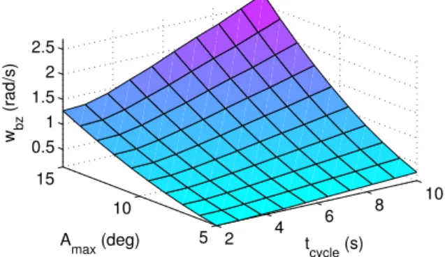
2 4 6 8 10 5 10 15 0.5 1 1.5 2 2.5 t_cycle (s) A_max (deg) w bz (rad/s)

Fig. 7. Dependence of the yaw rate to the period and amplitude of attitude angle reference trajectories.

This intuitive hypothesis is supported by our 3D model. Figure 7 illustrates the dependence of Ballbot’s yaw angular velocity to the period and amplitude of the attitude angle reference trajectory. As expected, there is significant yaw rotation associated with the circular motion of Ballbot in the workspace, increasing in magnitude as either the period or the amplitude of attitude angle trajectories increase. Our 3D model is the first model capable of incorporating this behavior into the dynamics. Even though one would be able to measure this change through inertial sensing and use feedback controllers to compensate, the inability of the underlying dynamics to model this behavior would inevitably manifest itself as inaccuracies in motion planning and exe-cution.

D. Characterizing External Variable Trajectories

As we noted before, one of the interesting but challenging features of the Ballbot morphology is its underactuated nature, which leads to task variables of interest (i.e. the robot position in W) being only indirectly controllable through the control of attitude angles. As shown in the example of Figure 5, our assumption that circular trajectories in the space of attitude angles would lead to circular trajectories is indeed observed in all of our simulations. In order to pin down the relation between trajectories in shape variables and trajectories in external variables, we ran simulations across a range of different attitude angle trajectories, varying the period tcycle and the maximum attitude angle Amax that

corresponds to the radius of the circular reference trajectory in attitude angle space. The reference trajectories for body

attitude degrees of freedom hence become

θx = Amaxsin(2πt/tcycle) (17)

θy = Amaxcos(2πt/tcycle) . (18)

2 4 6 8 10 5 10 15 1 2 3 4 5 t cycle (s) A max (deg) rpath (m) 2 4 6 8 10 5 10 15 1 2 3 t cycle (s) A max (deg) vpath (m/s)

Fig. 8. Dependence of the circular external variable trajectory parameters to the period and amplitude of the attitude reference trajectory. Left: radius of the circular path, Right: linear ball velocity along the circular path.

We ran simulations across the rangesAmax∈ [5, 15]deg

and tcycle ∈ [2, 10]s. We used the radii and linear

veloc-ities of the steady-state external variable trajectories as a parameterization of the ball path in W. Figure 8 shows our results, with the radius and velocity shown as a function of the reference trajectory period and amplitude on the left and right, respectively. It is also important to note that both the radius and velocity associated with these external variable trajectories are independent of the startup time and initial system states.

IV. CONCLUSION

In this paper, we proposed a new, three dimensional model of the Ballbot platform, which instantiates the recently introduced idea of mobility by rolling on spherical wheels. Our model captures interactions between the ground and the ball, as well as those between the ball and the robot body in such systems through several constraint equations corresponding to physical properties of such systems. In contrast to earlier attempts at modeling such systems that rely on decoupled planar approximations, our model has been able to capture important aspects of robot motion such as significant yaw rotations.

We have also proposed two different inverse-dynamics controllers, one for earlier, 2.5D models based on planar approximations, and one based on our novel 3D controller. We have shown that these controllers are capable of sus-taining dynamic behaviors such as circular trajectories in the workspace in a robust and stable fashion. In the context of such behaviors, we have shown that the controllers yield acceptable tracking performance for shape variables. We have also investigated the relation between circular motions in shape variables and characterized associated motions in external variables.

These results are the first steps towards dynamically dex-terous behavioral controllers and motion planners for the Ballbot platform. Unlike much of the previous work on

Ballbot platforms, our work aims to fully exploit dynamic properties of this system rather than restricting motion to states for which planar approximations remain accurate. A necessary next step in this direction is the experimental validation of this model and its possible extensions with more realistic friction models to increase its accuracy. Nev-ertheless, in the long run, we foresee that this 3D model and controllers based on this model will be valuable in the creation of accurate motion models for external variables of this system which are otherwise only indirectly controllable.

ACKNOWLEDGEMENTS

This work was partially supported by TUBITAK project 109E032.

REFERENCES

[1] P. S. Schenker, T. L. Huntsberger, P. Pirjanian, E. T. Baumgart-ner, and E. Tunstel, “Planetary rover developments supporting mars exploration, sample return and future human-robotic colonization,”

Autonomous Robots, vol. 14, no. 2, pp. 103–126, Mar. 2003.

[2] B. M. Yamauchi, “Packbot: a versatile platform for military robotics,” in Proceedings of SPIE: Unmanned Ground Vehicle Technology VI, vol. 5422, September 2004, pp. 228–237.

[3] U. Saranli, M. Buehler, and D. E. Koditschek, “RHex: A simple and highly mobile robot,” International Journal of Robotics Research, vol. 20, no. 7, pp. 616–631, July 2001.

[4] R. Playter, M. Buehler, and M. Raibert, “BigDog,” in Society of

Photo-Optical Instrumentation Engineers (SPIE) Conference Series, ser.

Presented at the Society of Photo-Optical Instrumentation Engineers (SPIE) Conference, vol. 6230, June 2006.

[5] E. Hale, N. Schara, J. Burdick, and P. Fiorini, “A minimally actu-ated hopping rover for exploration of celestialbodies,” in Robotics

and Automation, 2000. Proceedings. ICRA ’00. IEEE International

Conference on, vol. 1, San Francisco, CA, April 2000, pp. 420–427.

[6] T. Lauwers, G. Kantor, and R. Hollis, “One is enough!” in Robotics

Research, ser. Springer Tracts in Advanced Robotics, S. Thrun,

R. Brooks, and H. Durrant-Whyte, Eds. Springer Berlin / Heidelberg, 2007, vol. 28, pp. 327–336.

[7] M. Kumagai and T. Ochiai, “Development of a robot balanced on a ball - first report, implementation of the robot and basic control,”

Journal of Robotics and Mechatronics, vol. 22, no. 3, pp. 348–355,

2010.

[8] T. B. Lauwers, G. A. Kantor, and R. L. Hollis, “A dynamically stable single-wheeled mobile robot with inverse mouse-ball drive,” in Proc.

of the IEEE Int. Conf. on Robotics and Automation, Orlando, FL.,

May 2006, pp. 2884–2889.

[9] M. Kumagai and T. Ochiai, “Development of a robot balancing on a ball,” in Control, Automation and Systems, 2008. ICCAS 2008.

International Conference on, oct. 2008, pp. 433 –438.

[10] U. Nagarajan, G. Kantor, and R. Hollis, “Trajectory planning and con-trol of an underactuated dynamically stable single spherical wheeled mobile robot,” in Proc. of the IEEE Int. Conf. on Robotics and

Automation, may 2009, pp. 3743 –3748.

[11] U. Nagarajan, A. Mampetta, G. A. Kantor, and R. L. Hollis, “State transition, balancing, station keeping, and yaw control for a dynami-cally stable single spherical wheel mobile robot,” in Proc. of the IEEE

Int. Conf. on Robotics and Automation, may 2009, pp. 998 –1003.

[12] E. M. Schearer, “Modeling dynamics and exploring control of a single-wheeled dynamically stable mobile robot with arms,” Carnegie Mellon University, Tech. Rep. CMU-RI-TR-06-37, August 2006.

[13] U. Nagarajan, G. Kantor, and R. Hollis, “Hybrid control for navigation of shape-accelerated underactuated balancing systems,” in Proc. of the

IEEE Conf. on Decision and Control, dec. 2010, pp. 3566 –3571.

[14] U. Nagarajan, “Dynamic constraint-based optimal shape trajectory planner for shape-accelerated underactuated balancing systems,” in

Proc. of the Robotics, Science and Systems Conference, Zaragoza,