EUROPEAN ORGANIZATION FOR NUCLEAR RESEARCH (CERN)
CERN-EP-2018-307 2019/03/13
CMS-SUS-16-017
Inclusive search for supersymmetry in pp collisions at
√
s
=
13 TeV using razor variables and boosted object
identification in zero and one lepton final states
The CMS Collaboration
∗Abstract
An inclusive search for supersymmetry (SUSY) using the razor variables is performed using a data sample of proton-proton collisions corresponding to an integrated
lumi-nosity of 35.9 fb−1, collected with the CMS experiment in 2016 at a center-of-mass
energy of√s=13 TeV. The search looks for an excess of events with large transverse
energy, large jet multiplicity, and large missing transverse momentum. The razor kinematic variables are sensitive to large mass differences between the parent parti-cle and the invisible partiparti-cles of a decay chain and help to identify the presence of SUSY particles. The search covers final states with zero or one charged lepton and features event categories divided according to the presence of a high transverse mo-mentum hadronically decaying W boson or top quark, the number of jets, the number of b-tagged jets, and the values of the razor kinematic variables, in order to separate signal from background for a broad range of SUSY signatures. The addition of the boosted W boson and top quark categories within the analysis further increases the sensitivity of the search, particularly to signal models with large mass splitting be-tween the produced gluino or squark and the lightest SUSY particle. The analysis is interpreted using simplified models of R-parity conserving SUSY, focusing on gluino pair production and top squark pair production. Limits on the gluino mass extend to 2.0 TeV, while limits on top squark mass reach 1.14 TeV.
Published in the Journal of High Energy Physics as doi:10.1007/JHEP03(2019)031.
c
2019 CERN for the benefit of the CMS Collaboration. CC-BY-4.0 license ∗See Appendix A for the list of collaboration members
1
1
Introduction
We present an inclusive search for supersymmetry (SUSY) using the razor variables [1–3] on data collected by the CMS experiment in 2016. Supersymmetry extends space-time symmetry such that every fermion (boson) in the standard model (SM) has a bosonic (fermionic) part-ner [4–12]. Supersymmetric extensions of the SM yield solutions to the gauge hierarchy prob-lem without the need for large fine tuning of fundamental parameters [13–18], exhibit gauge coupling unification [19–24], and can provide weakly interacting particle candidates for dark matter [25, 26].
The search described in this paper is an extension of previous work presented in Refs. [2, 3]. The search is inclusive in scope, covering final states with zero or one charged lepton. To en-hance sensitivity to specific types of SUSY signatures, the events are categorized according
to the presence of jets consistent with high transverse momentum (pT) hadronically decaying
W bosons or top quarks, the number of identified charged leptons, the number of jets, and the
number of b-tagged jets. The search is performed in bins of the razor variables MRand R2[1–3].
The result presented in this paper is the first search for SUSY from the CMS experiment that incorporates both Lorentz-boosted and “non-boosted” (resolved) event categories. This search strategy provides broad sensitivity to gluino and squark pair production in R-parity [27] con-serving scenarios for a large variety of decay modes and branching fractions. The prediction of the SM background in the search regions (SRs) is obtained from Monte Carlo (MC) simula-tion calibrated with data control regions (CRs) that isolate the major background components. Additional validation of the assumptions made by the background estimation method yields estimates of the systematic uncertainties.
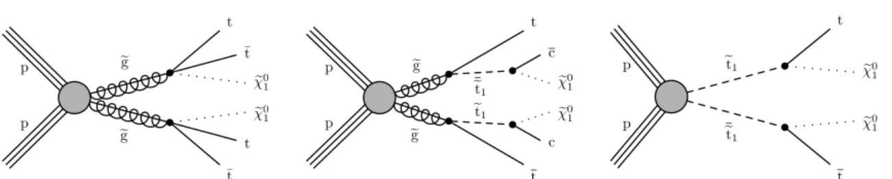
Other searches for SUSY by the CMS [28–36] and ATLAS [37–43] Collaborations have been performed using similar data sets and yield complementary sensitivity. Compared to those searches, the razor kinematic variables explore alternative signal-sensitive phase space and add robustness to the understanding of the background composition and the potential system-atic uncertainties in the background models. To give a characteristic example, for squark pair production with a squark mass of 1000 GeV and a neutralino mass of 100 GeV, we find that the overlap of signal events falling in the most sensitive tail regions of the razor kinematic variables and of other kinematic variables used in alternative searches described in Ref. [32] is 50–70%. We present interpretations of the results in terms of production cross section limits for several simplified models [44–47] for which this search has enhanced sensitivity. The simplified models considered include gluino pair production, with each gluino decaying to a pair of top quarks and the lightest SUSY particle (LSP), referred to as “T1tttt”; gluino pair-production, with each gluino decaying to a top quark and a low-mass top squark that subsequently decays to a charm quark and the LSP, referred to as “T5ttcc”; and top squark pair production, with each top squark decaying to a top quark and the LSP, referred to as “T2tt”. The corresponding diagrams for these simplified models are shown in Fig. 1. Although we only interpret the search results in a limited set of simplified models, the search can be sensitive to other simplified models that are not explicitly considered in this paper.
This paper is organized as follows. Details of the detector, trigger, and object reconstruction and identification are described in Section 2. The MC simulation samples used to model back-ground and signal processes are described in Section 3. The analysis strategy and event cate-gorization are discussed in Section 4, and the background modeling is discussed in Section 5. Systematic uncertainties are discussed in Section 6, and finally the results and interpretations are presented in Section 7. We summarize the paper in Section 8.
p p eg eg ¯ t t e χ01 e χ01 ¯t t p p eg eg et1 et1 t c e χ01 e χ01 c t p p et1 et1 t e χ01 e χ01 t
Figure 1: Diagrams for the simplified models considered in this analysis: (left) pair-produced gluinos, each decaying to two top quarks and the LSP, denoted T1tttt; (middle) pair-produced gluinos, each decaying to a top quark and a low mass top squark that subsequently decays to a charm quark and the LSP, denoted T5ttcc; (right) pair-produced top squarks, each decaying
to a top quark and the LSP, denoted T2tt. In the diagrams, the gluino is denoted byeg, the top
squark is denoted byet, and the lightest neutralino is denoted byχe
0
1and is the LSP.
2
The CMS detector and object reconstruction
The CMS detector consists of a superconducting solenoid of 6 m internal diameter, providing a magnetic field of 3.8 T. Within the solenoid volume there are a silicon pixel and a silicon strip tracker, a lead tungstate crystal electromagnetic calorimeter (ECAL), and a brass and scintillator hadron calorimeter (HCAL), each composed of a barrel and two endcap sections. Extensive forward calorimetry complements the coverage provided by the barrel and endcap detectors. Muons are measured in gas-ionization detectors embedded in the magnet steel flux-return yoke outside the solenoid. Events are selected by a two-level trigger system. The first level is based on a hardware filter, and the second level, the high level trigger, is implemented in software. A more detailed description of the CMS detector, together with a definition of the coordinate system used and the relevant kinematic variables, can be found in Ref. [48].
Physics objects are defined using the particle-flow (PF) algorithm [49], which aims to recon-struct and identify each individual particle in an event using an optimized combination of in-formation from the various elements of the CMS detector. Jets are clustered from PF candidates
using the anti-kT algorithm [50, 51] with a distance parameter of 0.4. Jet energy corrections are
derived from simulation and confirmed by in-situ measurements of the energy balance in dijet, multijet, photon+jet, and leptonically decaying Z+jet events [52]. Further details of the per-formance of the jet reconstruction can be found in Ref. [53]. Jets used in any selection of this
analysis are required to have pT >30 GeV and pseudorapidity|η| < 2.4. To identify jets
origi-nating from b quarks, we use the “medium” working point of the combined secondary vertex (CSVv2) b jet tagger, which uses an inclusive vertex finder to select b jets [54]. The efficiency to
identify a bottom jet is in the range of 50–65% for jets with pT between 20 and 400 GeV, while
the misidentification rate for light-flavor quark and gluon jets (charm jets) is about 1(10)%. We
also use the “loose” working point of the CSVv2 b jet tagger to identify b jets to be vetoed in the definition of various CRs. The loose b jet tagging working point has an efficiency of 80% and a misidentification rate for light-flavor and gluon jets of 10%.
Large-radius jets used for identifying Lorentz-boosted W bosons and top quarks are clustered
using the anti-kT algorithm with a distance parameter of 0.8. The subset of these jets having
|η| <2.4 and pT > 200 (400) GeV are used to identify W bosons (top quarks). Identification is
done using jet mass, the N-subjettiness variables [55], and subjet b tagging for top quarks. Jet mass is computed using the soft-drop algorithm [56], and is required to be between 65–105 and
3
105–210 GeV for W bosons and top quarks, respectively. The N-subjettiness variables:
τN =
1 d0
∑
kpT,kmin(∆R1,k,∆R2,k,· · · ,∆RN,k), (1)
where N denotes candidate axes for subjets, k runs over all constituent particles, and d0 =
R0∑kpT,k. R0 is the clustering parameter of the original jet, and ∆Rn,k is the distance from
constituent particle k to subjet n. The N-subjettiness variable is used to evaluate the consistency
of a jet with having N subjets. To enhance discrimination, the ratios τ21=τ2/τ1and τ32= τ3/τ2
are used for the W boson and top quark tagging, respectively, with the criteria of τ21<0.40 and
τ32 < 0.65. For tagging top quarks (“t tagging”), an additional requirement is imposed on the
subjet b tagging discriminant based on the multivariate CSVv2 algorithm [54]. The efficiencies for W boson and top quark tagging are on average 66 and 15%, respectively, with mistagging rates of 4.0 and 0.1% [53].
The missing transverse momentum vector~pmiss
T is defined as the projection of the negative
vector sum of the momenta of all reconstructed PF candidates on the plane perpendicular to
the beams. Its magnitude is referred to as pmissT . Events containing signatures consistent with
beam-induced background or anomalous noise in the calorimeters sometimes results in events
with anomalously large values of pmissT and are rejected using dedicated filters [57, 58]. The
performance of the pmissT at CMS may be found in Ref. [59].
Electrons are reconstructed by associating an energy cluster in the ECAL with a reconstructed track [60], and are identified on the basis of the electromagnetic shower shape, the ratio of energies deposited in the ECAL and HCAL, the geometric matching of the track and the calor-imeter cluster, the track quality and impact parameter, and isolation. To improve the efficiency for models that produce a large number of jets, a so-called “mini-isolation” technique is used, where the isolation cone shrinks as the momentum of the object increases. Further details are discussed in Ref. [2]. Muons are reconstructed by combining tracks found in the muon sys-tem with corresponding tracks in the silicon tracking detectors [61], and are identified based on the quality of the track fit, the number of detector hits used in the tracking algorithm, the compatibility between track segments, and isolation. Two types of selections are defined for electrons and muons: a “tight” selection with an average efficiency of about 70–75%, and a “loose” selection with an efficiency of about 90–95%. The loose selections are required to have
pT > 5 GeV, while the tight selections are required to have pT > 30 and 25 GeV for electrons
and muons, respectively. Similarly electrons (muons) are required to have|η| <2.5 (2.4), and
electrons with|η|(of 1.442–1.556) in the transition region between the barrel and endcap ECAL
are not considered because of limited electron reconstruction capabilities in that region.
Hadronically decaying τ leptons (τh) are reconstructed using the hadron-plus-strips
algo-rithm [62], which identifies τ lepton decay modes with one charged hadron and up to two neutral pions or three charged hadrons, and are required to be isolated. The “loose” selection
used successfully reconstructs τhdecays with an efficiency of about 50%. The reconstructed τh
leptons have pT>20 GeV and|η| <2.4.
Finally, photon candidates are reconstructed from energy clusters in the ECAL [63] and identi-fied based on the transverse shower width, the hadronic to electromagnetic energy ratio in the HCAL and ECAL, and isolation. Photon candidates that share the same energy cluster as an
identified electron are vetoed. Photons are used in the estimation of Z→νν+jets backgrounds,
and are required to have |η| < 2.5 and pT > 185 or 80 GeV for the non-boosted or boosted
3
Simulation
Monte Carlo simulated samples are used to predict the SM backgrounds in the SRs and to cal-culate the selection efficiencies for SUSY signal models. Events corresponding to the Z+jets,
γ+jets, and quantum chromodynamics (QCD) multijet background processes, as well as the
SUSY signal processes, are generated at leading order with MADGRAPH5 [email protected] [64,
65] interfaced withPYTHIAV8.205 [66] for fragmentation and parton showering, and matched
to the matrix element kinematic configuration using the MLM algorithm [67, 68]. The
CUETP8M1PYTHIA8 tune [69] was used. Other background processes are generated at
next-to-leading order (NLO) with MADGRAPH5 [email protected] [65] (W+jets, s-channel single top
quark, ttW, ttZ processes) or with POWHEG v2.0 [70–72] (tt+jets, t-channel single top quark,
and tW production), both interfaced with PYTHIA V8.205. Simulated samples generated at
LO (NLO) used the NNPDF3.0LO (NNPDF3.0NLO) [73] parton distribution functions. The
SM background events are simulated using a GEANT4-based model [74] of the CMS detector,
while SUSY signal events are simulated using the CMS fast simulation package [75]. All simu-lated events include the effects of pileup, multiple pp collisions within the same or neighboring bunch crossings.
The SUSY particle production cross sections are calculated to NLO plus next-to-leading-log (NLL) precision [76–81] with all other sparticles assumed to be heavy and decoupled. The NLO+NLL cross sections and their associated uncertainties from Ref. [81] are taken as a refer-ence to derive the exclusion limit on the SUSY particle masses.
To improve on the MADGRAPH5 aMC@NLOmodeling of the multiplicity of additional jets from
initial-state radiation (ISR), strongly produced SUSY signal samples are reweighted as a
func-tion of the number of ISR jets (NISR
jets). This correction is derived from a tt enriched control
sample such that the jet multiplicity from the MADGRAPH5 aMC@NLO-generated tt sample
agrees with data. The reweighting factors vary between 0.92 and 0.51 for NjetsISR between one
and six. We take one half of the deviation from unity as the systematic uncertainty in these reweighting factors.
4
Analysis strategy and event categorization
We perform the search in several event categories defined according to the presence of jets tagged as originating from a boosted hadronic W boson or top quark, the number of identified charged leptons, jets, and b-tagged jets. A summary of the categories used is shown in Table 1 below.
Events in the one-lepton category are required to have one and only one charged lepton
(elec-tron or muon), with pTabove 30 (25) GeV for electrons (muons) selected using the tight criteria,
while events in the zero-lepton category are required to have no electrons or muons passing
the loose selection criteria and no τhcandidates. One-lepton events are placed in the “Lepton
Multijet” category if they have between 4 and 6 jets, and placed in the “Lepton Seven-jet” cate-gory if they have 7 or more jets. One-lepton events with fewer than 4 jets are not considered in the analysis.
Zero-lepton events with jets tagged as originating from a boosted hadronic W boson or top quark decay are placed in a dedicated “boosted” event category. Events in this “boosted” category are analyzed separately with a set of CRs and validation tests specific for the analysis with boosted objects. They are further classified into those having at least one tagged W boson and one tagged b jet (“W” category), and those having at least one tagged top quark (“Top”
5
Table 1: Summary of the search categories, their charged lepton and jet count requirements, and the b tag bins that define the subcategories. Events passing the “Lepton veto” requirement
must have no electron or muon passing the loose selection, and no τhcandidate.
Category Lepton requirement Jet requirement b tag bins
Lepton multijet 1 “Tight” electron or muon 4–6 jets 0, 1, 2,≥3 b tags
Lepton seven-jet 1 “Tight” electron or muon ≥7 jets 0, 1, 2,≥3 b tags
Boosted W 4–5 jet Lepton veto ≥1 W-tagged jet ≥1 b tags
4–5 jets
Boosted W 6 jet Lepton veto ≥1 W-tagged jet ≥1 b tags
≥6 jets
Boosted top Lepton veto
0 W-tagged jets
≥0 b tags
≥1 t-tagged jet
≥6 jets
Dijet Lepton veto
0 W-tagged jets
0, 1,≥2 b tags
0 t-tagged jets 2–3 jets
Multijet Lepton veto
0 W-tagged jets
0, 1, 2,≥3 b tags
0 t-tagged jets 4–6 jets
Seven-jet Lepton veto
0W-tagged jets
0, 1, 2,≥3 b tags
0 t-tagged jets ≥7 jets
category). Events in the W category are further divided into subcategories with 4–5 jets, and 6 jets or more. Zero-lepton events not tagged as having boosted W bosons or top quarks are placed into the “Dijet” category if they have two or three jets, the “Multijet” category if they have between 4 and 6 jets, and into the “Seven-jet” category if they have 7 or more jets.
The Dijet category is further divided into subcategories with zero, one, and two or more b-tagged jets, and all other non-boosted categories are divided into subcategories with zero, one, two, and three or more b-tagged jets.
For each event in the above categories, we group the selected charged leptons and jets in the event into two distinct hemispheres called megajets, whose four-momenta are defined as the vector sum of the four-momenta of the physics objects in each hemisphere. The clustering algorithm selects the grouping that minimizes the sum of the squared invariant masses of the
two megajets [82]. We define the razor variables MRand MRT as:
MR≡ q (|~pj1| + |~pj2|)2− (pj1 z +pjz2)2, (2) MRT ≡ s pmiss T (p j1 T+p j2 T) − ~pTmiss· (~p j1 T + ~p j2 T) 2 , (3) where~pji, ~pji T, and p ji
z are the momentum of the i-th megajet, its transverse component with
respect to the beam axis, and its longitudinal component, respectively. The dimensionless vari-able R is defined as:
R≡ M
R T
MR
. (4)
For pair-produced SUSY signals, the variable MR quantifies the mass splitting between the
pair-produced particle and the LSP, and exhibits a peaking structure, while for background it is distributed as an exponentially decaying spectrum. The variable R quantifies the degree of imbalance between the visible and invisible decay products and helps to suppress backgrounds which do not produce any weakly interacting particles. The combination of the two variables provide powerful discrimination between the SUSY signal and SM backgrounds.
Single-electron or single-muon triggers are used to collect events in the one-lepton categories,
with a total trigger efficiency of about 80% for reconstructed pT around 30 GeV, growing to
95% for reconstructed pT above 50 GeV. Events in the boosted category are collected using
triggers that select events based on the pT of the leading jet and the scalar pT sum of all jets,
HT. The trigger efficiency is about 50% at the low range of the MRand R2kinematic variables
and grows to 100% for MR > 1.2 TeV and R2 > 0.16. For the zero-lepton non-boosted event
categories, dedicated triggers requiring at least two jets with pT >80 GeV and loose thresholds
on the razor variables MRand R2 are used to collect the events. The trigger efficiency ranges
from 95–100% and increases with MRand R2.
Preselection requirements on the MRand R2 variables are made depending on the event
cate-gory. For events in the one-lepton categories, further requirements are made on the transverse
mass mTdefined as follows:
mT =
q 2pmiss
T p`T[1−cos(∆φ)], (5)
where p`
T is the charged-lepton transverse momentum, and ∆φ is the azimuthal angle (in
ra-dians) between the charged-lepton momentum and the pmissT . For events in the zero-lepton
categories, further requirements are made on the azimuthal angle∆φRbetween the axes of the
7
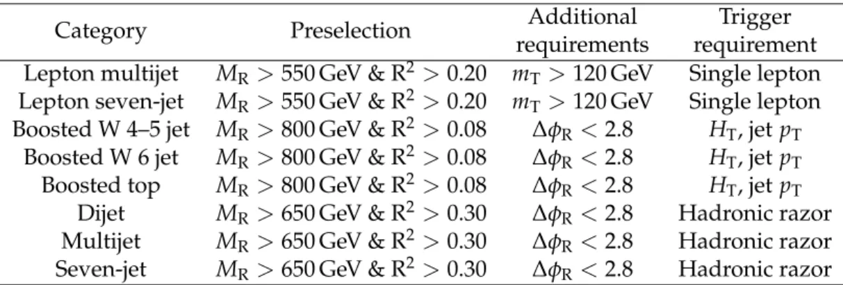
Table 2: The baseline requirements on the razor variables MRand R2, additional requirements
on mTand∆φR, and the trigger requirements are shown for each event category.
Category Preselection Additional Trigger
requirements requirement
Lepton multijet MR >550 GeV & R2>0.20 mT >120 GeV Single lepton
Lepton seven-jet MR >550 GeV & R2>0.20 mT >120 GeV Single lepton
Boosted W 4–5 jet MR >800 GeV & R2>0.08 ∆φR <2.8 HT, jet pT
Boosted W 6 jet MR >800 GeV & R2>0.08 ∆φR <2.8 HT, jet pT
Boosted top MR >800 GeV & R2>0.08 ∆φR <2.8 HT, jet pT
Dijet MR >650 GeV & R2>0.30 ∆φR <2.8 Hadronic razor
Multijet MR >650 GeV & R2>0.30 ∆φR <2.8 Hadronic razor
Seven-jet MR >650 GeV & R2>0.30 ∆φR <2.8 Hadronic razor
Finally, in each event category, the search is performed in bins of the kinematic variables MR
and R2 in order to take advantage of the varying signal-to-background ratio in the different
bins. For one-lepton categories, the SRs are composed of five bins in MR, starting from 550 GeV,
and five bins in R2starting from 0.20. For the zero-lepton boosted categories, the SRs are
com-posed of five bins in MR, starting from 800 GeV, and five bins in R2, starting from 0.08. Finally,
for the zero-lepton non-boosted categories, the SRs are composed of five bins in MR, starting
from 650 GeV, and four bins in R2starting from 0.30. To match with the expected resolution, the
bin widths in MRincreases from 100 to 300 GeV as the value of MRgrows from 400 to 1200 GeV.
In each category, to limit the impact of statistical uncertainties due to the limited size of the MC simulation samples, bins are merged such that the expected background in each bin is larger than about 0.1 events. As a result, the SRs have a decreasing number of bins as the number of
jets, b-tagged jets, and MRincreases.
5
Background modeling
The main background processes in the SRs considered are W(`ν)+jets (with` =e, µ, τ), Z(νν)+jets,
tt, and QCD multijet production. For event categories with zero b-tagged jets, the background
is primarily composed of the W(`ν)+jets and Z(νν)+jets processes, while for categories with
two or more b-tagged jets it is dominated by the tt process. There are also small contribu-tions at the level of a few percent from single top quark production, production of two or three electroweak bosons, and production of tt in association with a W or Z boson.
The background prediction strategy relies on the use of CRs to isolate each background pro-cess, address deficiencies of the MC simulation using control samples in data, and estimate systematic uncertainties in the expected event yields. The CRs are defined such that they have no overlap with any SRs. For the dominant backgrounds discussed above, the primary sources of mismodeling come from inaccuracy in the MC prediction of the hadronic recoil spectrum
and the jet multiplicity. Corrections to the MC simulation are applied first in bins of MR and
R2, and then subsequently in the number of jets (N
jets) to address these modeling inaccuracies.
The CR bins generally follow the bins of the SRs described in Section 4, but bins with limited statistical power are merged in order to avoid large statistical fluctuations in the background predictions.
For the boosted categories, the CR selection and categorization are slightly adapted and the de-tails are discussed further in Section 5.4. An additional validation of the background prediction method is also performed for the boosted categories.
In what follows, all background MC samples are corrected for known mismodeling of the jet energy response, the trigger efficiency, and the selection efficiency of electrons, muons, and b-tagged jets. These corrections are mostly in the range of 0–5%, but can be as large as 10% in
bins with large MRand R2, where the corrections have larger statistical uncertainties.
5.1 The tt and W
(`
ν)
+jets backgroundsWe predict the tt and W(`ν)backgrounds from the MC simulation corrected for inaccuracies
in the modeling of the hadronic recoil. The corrections are derived in a CR consisting of events having at least one tight electron or muon. In order to separate the CR from the SRs and to
reduce the QCD multijet background, the pmissT is required to be larger than 30 GeV, and mT is
required to be between 30 and 100 GeV.
The tight lepton control sample is separated into W(`ν)+jets-enriched and tt-enriched samples
by requiring events to have zero (for W(`ν)+jets), or one or more (for tt) b-tagged jets,
respec-tively. The purity of the W(`ν)+jets and tt dominated CRs are both about 80%. In each sample,
corrections to the MC prediction are derived in two-dimensional bins in MRand R2. The
con-tribution from all other background processes estimated from simulation in each bin in a given
CR (NCR bin iMC,bkg) is subtracted from the data yield in the corresponding bin in the CR (NCR bin idata ),
and compared to the MC prediction (NCR bin iMC,tt ) to derive the correction factor:
Cttbin i= N data CR bin i−N MC,bkg CR bin i NCR bin iMC,tt . (6)
Finally, the prediction for the tt background in the SR (NSR bin itt ) is:
NSR bin itt = NSR bin iMC,tt Cttbin i, (7)
where NSR bin iMC,tt is the prediction for the SR from the MC simulation.
Because the tt-enriched sample is the purer of the two, the corrections are first derived in this
sample. These corrections are applied to the tt simulation in the W(`ν)+jets-enriched sample,
and then analogous corrections and predictions for the W(`ν)+jets background process are
derived.
The corrections based on MRand R2are measured and applied by averaging over all jet
mul-tiplicity bins. As our SRs are divided according to the jet mulmul-tiplicity, additional corrections are needed in order to ensure correct background modeling for different numbers of jets. We
derive these corrections separately for the tt and W(`ν)+jets samples, obtaining correction
fac-tors for events with two or three jets, four to six jets, and seven or more jets. The tt correction
is derived prior to the W(`ν)+jets correction to take advantage of the slightly higher purity of
the tt CR.
We also check for MC mismodeling that depends on the number of b jets in the event. To do
this we apply the above-mentioned corrections in bins of MR, R2, and the number of jets and
derive an additional correction needed to make the predicted MRspectrum match that in data
for each b tag multiplicity. This correction is performed separately for events with two or three, four to six, and seven or more jets.
A final validation of the MC modeling in this tight lepton CR is completed by comparing the R2
spectrum in data with the MC prediction in each jet multiplicity and b tag multiplicity category.
5.2 TheZ→νν background 9
uncertainty in the data-to-MC ratio in each bin of R2 as a systematic uncertainty in the tt and
W+jets backgrounds in the analysis SRs.
The tt background in the tight lepton CR is composed mostly of lepton+jets tt events, where one top quark decayed fully hadronically and the other top quark decayed leptonically. In the
leptonic analysis SRs, the mTrequirement suppresses lepton+jets tt events, and the dominant
remaining tt background consists of tt events where both top quarks decayed leptonically, and one of the two leptons is not identified. It is therefore important to validate that the corrections to the tt simulation derived in the tight lepton CR also describe dileptonic tt events well. We perform this check by selecting an event sample enriched in dileptonic tt events, applying the corrections on the tt simulation prediction derived in the tight lepton CR, and evaluating the consistency of the data with the corrected prediction. This check is performed separately for each jet multiplicity category used in the analysis SRs. The dilepton tt-enriched sample consists
of events with two tight electrons or muons with pT > 30 GeV and invariant mass larger than
20 GeV, at least one b-tagged jet with pT>40 GeV, and pmissT >40 GeV. Events with two
same-flavor leptons with invariant mass between 76 and 106 GeV are rejected to suppress Drell–
Yan background. The pmissT and the mT variables are computed treating one of the leptons in
each event as visible and the other as invisible, and the requirement on the mTis subsequently
applied. A systematic uncertainty in the dilepton tt background is assessed by comparing
data with the MC prediction in the MRdistribution for each jet multiplicity category. The MR
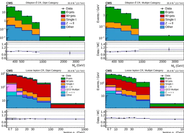
distributions in the tt dilepton CR for the two to three and four to six jet event categories are displayed in the upper row of Fig. 2.
The MC prediction for the hadronic SRs can be affected by potential mismodeling of the
iden-tification efficiency for electrons, muons, and τh candidates. The loose lepton and τh CRs are
defined in order to assess the modeling of this efficiency in simulation. Events in the loose
lepton (τh) CR are required to have at least one loose electron or muon (τhcandidate) and pass
one of the hadronic razor triggers. These events must also have mT between 30 and 100 GeV,
MR > 400 GeV, R2 > 0.25, and at least two jets with pT > 80 GeV. The data and MC
predic-tion are compared in bins of lepton pT and η for each jet multiplicity category. A systematic
uncertainty of about 25% is assigned to cover the difference between data and prediction in
the lepton pT spectrum. No further systematic mismodeling is observed in the lepton η
dis-tributions, and the size of the uncertainty in each η bin is propagated as an uncertainty in the
analysis SR predictions. The lepton pT distributions obtained in the loose lepton CR for the
categories with two to three and four to six jets are displayed in the lower row of Fig. 2.
5.2 The Z
→
νν backgroundThe background prediction for the Z(νν)+jets process is made using the same methodology as
for the tt and W(`ν) background processes. We take advantage of the kinematic similarities
between the Z → ``, W(`ν)+jets, and γ+jets processes [83–85]. Corrections to the hadronic
recoil and jet multiplicity spectra are obtained in a control sample enriched in γ+jets events, and
the validity of these corrections is checked in a second control sample enriched in W(`ν)+jets
events. A third control sample, enriched in Z → ``events, is used to normalize the obtained
correction factors and to provide an additional consistency check of the MC prediction.
The γ+jets control sample consists of events having at least one selected photon and passing a
set of kinematic requirements. Photons are required to have pT >185 GeV and pass loose
iden-tification and isolation criteria. The photon is treated as invisible—its pTis added vectorially to
the~pTmiss, and it is ignored in the calculation of MR—in order to simulate the invisible Z boson
[GeV] R M Events / GeV 2 − 10 1 − 10 1 10 Data +jets t t W+jets Single t ll → Z Other (13 TeV) -1 35.9 fb
CMS Dilepton tt CR, Dijet Category
(GeV) R M 400 500 1000 2000 3000 Data / MC 0.6 0.8 1 1.2 1.4 MR [GeV] Events / GeV 2 − 10 1 − 10 1 Data +jets t t W+jets Single t ll → Z Other (13 TeV) -1 35.9 fb
CMS Dilepton tt CR, Multijet Category
(GeV) R M 400 500 1000 2000 3000 Data / MC 0.6 0.8 1 1.2 1.4 [GeV] T lepton p Events / GeV 10 2 10 3 10 Data +jets t t W+jets Single t ll → Z QCD Multijet ν ν → Z Other (13 TeV) -1 35.9 fb
CMS Loose lepton CR, Dijet Category
(GeV) T lepton p 6 7 10 20 30 100 200 1000 Data / MC 0.6 0.8 1 1.2 1.4 [GeV] T lepton p Events / GeV 10 2 10 Data +jets t t W+jets Single t ll → Z QCD Multijet ν ν → Z Other (13 TeV) -1 35.9 fb
CMS Loose lepton CR, Multijet Category
(GeV) T lepton p 6 7 10 20 30 100 200 1000 Data / MC 0.6 0.8 1 1.2 1.4
Figure 2: The MRdistribution in the tt dilepton CR (upper row) and lepton pT distribution in
the loose lepton CR (lower row) are displayed in the 2–3 (left) and 4–6 (right) jet categories along with the corresponding MC predictions. The corrections derived from the tt and W+jets CR have been applied. The ratio of data to the MC prediction is shown on the bottom panel, with the statistical uncertainty expressed through the data point error bars and the systematic uncertainty in the background prediction represented by the shaded region.
5.2 TheZ→νν background 11 ll) (GeV) → (Invisible Z R M Events / GeV 2 − 10 1 − 10 1 10 Data ll → Z +jets t t W+jets Single t Other (13 TeV) -1 35.9 fb
CMS Drell-Yan Dilepton CR, Dijet Category
ll) (GeV) → (Invisible Z R M 500 1000 2000 3000 4000 Data / MC 0.6 0.8 1 1.2 1.4 MR (Invisible Z → ll) (GeV) Events / GeV 1 − 10 1 10 Data ll → Z +jets t t W+jets Single t Other (13 TeV) -1 35.9 fb
CMS Drell-Yan Dilepton CR, Multijet Category
ll) (GeV) → (Invisible Z R M 500 1000 2000 3000 4000 Data / MC 0.6 0.8 1 1.2 1.4
Figure 3: The MRdistribution in the Z→ ``+jets CR is displayed in the 2–3 (left) and 4–6 (right)
jet categories along with the corresponding MC predictions. The corrections derived from the
γ+jets CR, as well as the overall normalization correction, have been applied in this figure.
two jets with pT >80 GeV, and have MR>400 GeV and R2 >0.25.
The contribution of misidentified photons to the yield in this control sample is estimated via
a template fit to the distribution of the photon charged isolation, the pT sum of all charged PF
particles within a∆R cone of size 0.4 centered on the photon momentum axis. The fit is
per-formed in bins of MRand R2and yields an estimate of the purity of the photon sample in each
bin. Contributions from other background processes such as ttγ are estimated using simula-tion and account for about 1–2%. Addisimula-tionally, events in which the photon is produced within a jet are considered to be background. Corrections to the hadronic recoil in simulation are de-rived in this CR by subtracting the estimated background yields from the number of observed counts, and comparing the resulting yield with the prediction from the γ+jets simulation, in
each bin of MRand R2.
As in the tight lepton CR described in Section 5.1, an additional correction is derived to account for possible mismodeling in simulation as a function of the jet multiplicity. This correction is derived for events with two or three jets, with four to six jets, and with seven or more jets. After these corrections are applied, the data in the CR are compared with the MC prediction
in bins of the number of b-tagged jets. As in the tight lepton CR, the MRspectra in simulation
are corrected to match the data in each b tag category, and a systematic uncertainty in the
Z(νν)+jets background is assigned based on the size of the uncertainty in each bin of R2.
A check of the Z(νν)+jets prediction is performed with a sample enriched in Z → `` decays.
Events in this sample are required to have two tight electrons or two tight muons having an invariant mass consistent with the Z mass. The two leptons are treated as invisible for the pur-pose of computing the razor variables. Events must have no b-tagged jets, two or more jets
with pT > 80 GeV, MR > 400 GeV, and R2 > 0.25. The correction factors obtained from the
γ+jets CR are normalized so that the total MC prediction in the Z → `+`−+jets CR matches
the observed data yield. This corrects for the difference between the true γ+jets cross section
and the leading order cross section used to normalize the simulated samples. The MR
distri-butions in this CR for the two to three and four to six jet categories are shown in Fig. 3. The
observed residual disagreements between data and simulation in the MR and R2distributions
are propagated as systematic uncertainties in the Z(νν)+jets prediction.
The MC corrections derived in the γ+jets CR are checked against a second set of corrections
derived in a CR enriched in W(`ν)+jets events. This CR is identical to the W(`ν)+jets sample
computing MRand R2. Correction factors are derived in the same way as in the W(`ν)+jets CR.
The full difference between these corrections and those obtained from the γ+jets CR is taken
as a systematic uncertainty in the Z(νν)+jets prediction in the SR, and is typically between
10 and 20%, depending on the bin.
5.3 The QCD multijet background
Multijet events compose a nonnegligible fraction of the total event yield in the hadronic SRs. Such events are characterized by a significant undermeasurement of the energy of a jet, and
consequently a large amount of pmissT , usually pointing towards the mismeasured jet. A large
fraction of QCD multijet events are rejected by the requirement that the azimuthal angle∆φR
between the axes of the two razor megajets is less than 2.8. We treat the events with∆φR ≥2.8
as a CR of QCD multijet events, while the events with∆φR<2.8 define the SRs.
We estimate the number of QCD multijet events in this CR in bins of MRand R2by subtracting
the predicted contribution of other processes from the total event yield in each bin. This is done for each jet multiplicity category. We observe in simulation that the fraction of QCD multijet
events at each b tag multiplicity is independent of MR, R2, and ∆φR. The event yields in the
QCD CRs are therefore measured inclusively in the number of b tags and then scaled according to the fraction of QCD multijet events at each multiplicity of b-tagged jets.
We then predict the number of QCD multijet events in the SRs via the transfer factor ζ, defined as
ζ = N(|∆φR| <2.8)
N(|∆φR| >2.8). (8)
It is calculated using control regions in data and validated with simulation. The QCD
back-ground prediction in each bin (NSR bin iQCD ) is made as:
NSR bin iQCD =ζ(NCR bin idata −NCR bin ibkg ), (9)
where NCR bin idata is the number of events observed in the data CR and NCR bin ibkg is the contribution
from background processes other than the QCD multijet process and is predicted from the corrected MC.
We observe in simulation that ζ changes slowly with MRand increases roughly linearly with
R2. In data we therefore compute ζ in bins of MRand R2in a low-R2region defined by 0.20 <
R2 < 0.30 and fit the computed values with a linear function in MR and R2. We then use the
linear fit and its uncertainty to estimate the value of ζ in the analysis SRs. The fit is performed separately in each category of jet multiplicity, but inclusively in the number of b-tagged jets, as ζ is observed in simulation not to depend on the b tag multiplicity. For the category with
seven or more jets, the fit function is allowed to depend on R2only, because of the low number
of events in the fit region.
The statistical uncertainty in the CR event counts and the fitted uncertainty of the transfer fac-tor extrapolation are propagated as systematic uncertainties of the QCD multijet background prediction. Another systematic uncertainty of 30% is propagated in order to cover the depen-dence of the transfer factor on the number of b-tagged jets in different CRs. Furthermore, we
make an alternative extrapolation for the transfer factor where we allow a dependence on MR
and R2for the Seven-jet category, and a quadratic dependence on M
Rfor the Dijet and Multijet
categories. The difference in the QCD multijet background prediction between the default and alternative transfer factor extrapolation is propagated as an additional systematic uncertainty,
5.4 Background modeling in boosted event categories 13
5.4 Background modeling in boosted event categories
The dominant SM background processes in the boosted categories are the same as in the non-boosted categories. An additional, but important source of background comes from processes where one of the jets in the event is mistagged as a boosted hadronic W boson or top quark. Requiring boosted objects in the selection results in a smaller number of events in the SRs or CRs. As a general rule, in cases where no MC events exist in SR bins for a given background process, MC counts in these bins are extrapolated from a looser version of the signal selection obtained by relaxing the N-subjettiness criteria for W or t tagging. For cases where there are no counts or very low statistical precision in the CR bins, these depleted bins are temporarily merged to obtain coarser bins with increased event count. Background estimation is done in two steps, where first the yields are estimated using the coarser bins, and next, the yields in coarse bins are distributed to the finer bins proportional to the background MC counts in the finer bins.
5.4.1 The tt+jets and W+jets background estimation for the boosted categories
The CRs for the tt and W+jets backgrounds are defined similar to the CRs used for the non-boosted categories. We require exactly one loose electron or muon. To suppress contamination
from signal processes, mT is required to be less than 100 GeV. To mimic the signal selection,
the∆φR < 2.8 requirement is applied. To estimate the top quark background for the boosted
W 4–5 jet and boosted W 6 jet SR categories, we require events in the CR to have at least one boosted W boson and one b-tagged jet, while for the boosted top category, we require
one boosted top quark. To estimate the W(`ν)+jets background for the boosted W 4–5 jet and
boosted W 6 jet SR categories, we require events in the CR to have no loosely tagged b jets, while for the boosted top category we require no b-tagged subjets. To maintain consistency with SR kinematics, we require a jet which is tagged only using the W boson or top quark mass requirement, but without the N-subjettiness requirement. The background estimate for each SR i is then extrapolated from the corresponding CR via transfer factors calculated in MC:
λi = NiSR,MC/NiCR,MC.
For certain bins, the MC prediction of the transfer factors can have large statistical fluctuations from the limited number of MC events. To smooth out these fluctuations we use a combination of bin-merging and extrapolations from a region with looser requirements on the N-subjettiness variables. While the fluctuations in the nominal background prediction are smoothed out, the statistical uncertainties from the limited MC sample size are still propagated as a systematic uncertainty.
Figure 4 shows the b-tagged jet multiplicity distribution, identified with the medium b jet tag-ger, for events in the boosted W 6 jet category in the tt CR before applying the b tagging
se-lection, and the mT distribution in the boosted top category in the tt CR before applying the
mT selection. Figure 5 shows the distribution in MR and R2bins for events in the boosted top
category in the tt CR, and for events in the boosted W 4–5 jet and boosted W 6 jet categories in
the W(`ν)+jets CR. The purity of tt+jets and single top events in the tt CR is more than 80%,
and the purity of the W(`ν)+jets process in the W(`ν)+jets CR is also larger than 80%.
5.4.2 The Z→νν+jets background estimation for the boosted categories
The background estimate for the Z → νν+jets process is again similar to the method used for
the non-boosted categories. We make use of the similarity in the kinematics of the photon in
γ+jets events and the Z boson in Z+jets events to select a control sample of γ+jets to mimic
b N 0 1 2 3 4 5 6 Events / bin 1 − 10 1 10 2 10 3 10 4 10 W 6 jet category control region, t t Data tt+jets W+jets Single t Other CMS -1 (13 TeV) 35.9 fb b N 0 1 2 3 4 5 6 Data/MC 0 1 2
Stat. unc. Stat. + syst. unc. (GeV)
T m 0 50 100 150 200 250 300 350 400 450 500 Events / bin 1 − 10 1 10 2 10 3 10 4 10 Top category control region, t t Data tt+jets Single t W+jets Other CMS -1 (13 TeV) 35.9 fb (GeV) T m 0 50 100 150 200 250 300 350 400 450 500 Data/MC 0 1 2 3 4 5
Stat. unc. Stat. + syst. unc.
Figure 4: The distribution of b-tagged jet multiplicity before applying the b tagging selection
requirement in the tt CR of the boosted W 6 jet category (left), and the distribution in mT
be-fore applying the mTselection requirement in the tt CR of the boosted top category (right) are
shown. The ratio of data over MC prediction is shown in the lower panels, where the gray band is the total uncertainty and the dashed band is the statistical uncertainty in the MC prediction.
with pT > 80 GeV from data collected by jet and HT triggers. The momentum of the photon
is added to~pTmiss to mimic the contribution of the neutrinos from Z → ννdecays. We require
that the events contain no loose leptons or τhcandidates, and∆φR, computed after treating the
photon as invisible, is required to be less than 2.8. One W-tagged or t-tagged jet is required
for the boosted W and top categories, respectively. Figure 6 shows the MR–R2distribution for
the boosted top category. The QCD multijet contribution to the γ+jets CR is accounted for by
a template fit to the photon charged isolation variable in inclusive bins of MR and R2. Other
background processes in the γ+jets CRs are small and predicted using MC. Finally, the SR
prediction for the Z → νν+jets background is extrapolated from the γ+jets yields via the MC
transfer factor λZ→νν = N
SR,MC
Z→νν /N
CR,MC
γ+jets .
We perform a cross check on the previous estimate using a CR enhanced in Z → `` events.
The Z→ ``CR is defined by requiring exactly two tight electrons or muons with pT >10 GeV
and dilepton mass satisfying|m``−mZ| < 10 GeV, where mZ is the Z boson mass. All other
requirements are the same as those for the γ+jets CR. The momentum of the dilepton system
is added vectorially to~pmiss
T to mimic an invisible decay of the Z boson. Similarly for the
non-boosted categories, the comparison between data and MC yields in the Z → ``CR are used to
correct the MC transfer factor λ to account for the impact of missing higher order corrections on the total normalization predicted by the γ+jets simulation.
As for the inclusive categories, we obtain an alternative estimate from the W(→ `ν)
+jets-enriched CR to validate the predictions from the γ+jets CR. We require the presence of exactly
one tight electron or muon. mT is required to be between 30 and 100 GeV. The rest of the
se-lection is the same as for the γ+jets CR. The lepton momentum is added vectorially to~pmiss
T to
mimic an invisible decay. The W(→ `ν)+jets CR yields are extrapolated to the SR via transfer
factors calculated from simulation to obtain the alternative Z→ νν+jets background estimate.
Figure 7 compares the estimates from the γ+jets CR, the W(→ `ν)+jets CR, and the MC
5.4 Background modeling in boosted event categories 15 2 R [0.08, 0.12] [0.12, 0.16] [0.16, 0.24] [0.24, 0.40] [0.40, 1.50] [0.08, 0.12] [0.12, 0.16] [0.16, 0.24] [0.24, 0.40] [0.40, 1.50] [0.08, 0.12] [0.12, 0.16] [0.16, 0.24] [0.24, 0.40] [0.40, 1.50] [0.08, 0.12] [0.12, 0.16] [0.16, 0.24] [0.24, 1.50] [0.08, 0.12] [0.12, 0.16] [0.16, 1.50] Events / bin 1 − 10 1 10 2 10 3 10 4 10 W 4-5 jet category W+jets control region,
Data W+jets X t VV(V)+t +jets t t Single t Multijet Other CMS -1 (13 TeV) 35.9 fb (TeV) R M [0.8, 1] [1, 1.2] [1.2, 1.6] [1.6, 2] [2, 4] [4, 0] 2 R [0.08, 0.12] [0.12, 0.16] [0.16, 0.24] [0.24, 0.40] [0.40, 1.50] [0.08, 0.12] [0.12, 0.16] [0.16, 0.24] [0.24, 0.40] [0.40, 1.50] [0.08, 0.12] [0.12, 0.16] [0.16, 0.24] [0.24, 0.40] [0.40, 1.50] [0.08, 0.12] [0.12, 0.16] [0.16, 0.24] [0.24, 1.50] [0.08, 0.12] [0.12, 0.16] [0.16, 1.50] Data/MC 0 1 2 3
Stat. unc. Stat. + syst. unc.
2 R [0.08, 0.12] [0.12, 0.16] [0.16, 0.24] [0.24, 0.40] [0.40, 1.50] [0.08, 0.12] [0.12, 0.16] [0.16, 0.24] [0.24, 0.40] [0.40, 1.50] [0.08, 0.12] [0.12, 0.16] [0.16, 0.24] [0.24, 0.40] [0.40, 1.50] [0.08, 0.12] [0.12, 0.16] [0.16, 0.24] [0.24, 1.50] [0.08, 0.12] [0.12, 0.16] [0.16, 1.50] Events / bin 1 − 10 1 10 2 10 3 10 4 10 W 6 jet category W+jets control region,
Data W+jets +jets t t X t VV(V)+t Single t Multijet Other CMS -1 (13 TeV) 35.9 fb (TeV) R M [0.8, 1] [1, 1.2] [1.2, 1.6] [1.6, 2] [2, 4] [4, 0] 2 R [0.08, 0.12] [0.12, 0.16] [0.16, 0.24] [0.24, 0.40] [0.40, 1.50] [0.08, 0.12] [0.12, 0.16] [0.16, 0.24] [0.24, 0.40] [0.40, 1.50] [0.08, 0.12] [0.12, 0.16] [0.16, 0.24] [0.24, 0.40] [0.40, 1.50] [0.08, 0.12] [0.12, 0.16] [0.16, 0.24] [0.24, 1.50] [0.08, 0.12] [0.12, 0.16] [0.16, 1.50] Data/MC 0 1 2 3 4 5
Stat. unc. Stat. + syst. unc.
2 R [0.08, 0.12] [0.12, 0.16] [0.16, 0.24] [0.24, 0.40] [0.40, 1.50] [0.08, 0.12] [0.12, 0.16] [0.16, 0.24] [0.24, 0.40] [0.40, 1.50] [0.08, 0.12] [0.12, 0.16] [0.16, 0.24] [0.24, 0.40] [0.40, 1.50] [0.08, 0.12] [0.12, 0.16] [0.16, 0.24] [0.24, 1.50] [0.08, 0.12] [0.12, 0.16] [0.16, 1.50] Events / bin 1 − 10 1 10 2 10 3 10 4 10 Top category control region, t t Data tt+jets Single t W+jets X t VV(V)+t Other CMS -1 (13 TeV) 35.9 fb (TeV) R M [0.8, 1] [1, 1.2] [1.2, 1.6] [1.6, 2] [2, 4] [4, 2.8e-320] 2 R [0.08, 0.12] [0.12, 0.16] [0.16, 0.24] [0.24, 0.40] [0.40, 1.50] [0.08, 0.12] [0.12, 0.16] [0.16, 0.24] [0.24, 0.40] [0.40, 1.50] [0.08, 0.12] [0.12, 0.16] [0.16, 0.24] [0.24, 0.40] [0.40, 1.50] [0.08, 0.12] [0.12, 0.16] [0.16, 0.24] [0.24, 1.50] [0.08, 0.12] [0.12, 0.16] [0.16, 1.50] Data/MC 0 1 2 3
Stat. unc. Stat. + syst. unc.
Figure 5: MR–R2 distributions in the W+jets CRs of the boosted W 4–5 jet (upper left) and
boosted W 6 jet (upper right) categories, and the tt CR (lower) of the boosted top category. The ratio of data over MC prediction is shown in the lower panels, where the gray band is the total uncertainty and the dashed band is the statistical uncertainty in the MC prediction.
2 R [0.08, 0.12] [0.12, 0.16] [0.16, 0.24] [0.24, 0.40] [0.40, 1.50] [0.08, 0.12] [0.12, 0.16] [0.16, 0.24] [0.24, 0.40] [0.40, 1.50] [0.08, 0.12] [0.12, 0.16] [0.16, 0.24] [0.24, 0.40] [0.40, 1.50] [0.08, 0.12] [0.12, 0.16] [0.16, 0.24] [0.24, 1.50] [0.08, 0.12] [0.12, 0.16] [0.16, 1.50] Events / bin 1 − 10 1 10 2 10 3 10 4 10 5 10 W 4-5 jet category +jets control region,
γ Data γ+jets Multijet Other CMS 35.9 fb-1 (13 TeV) (TeV) R M [0.8, 1] [1, 1.2] [1.2, 1.6] [1.6, 2] [2, 4] [4, 0] 2 R [0.08, 0.12] [0.12, 0.16] [0.16, 0.24] [0.24, 0.40] [0.40, 1.50] [0.08, 0.12] [0.12, 0.16] [0.16, 0.24] [0.24, 0.40] [0.40, 1.50] [0.08, 0.12] [0.12, 0.16] [0.16, 0.24] [0.24, 0.40] [0.40, 1.50] [0.08, 0.12] [0.12, 0.16] [0.16, 0.24] [0.24, 1.50] [0.08, 0.12] [0.12, 0.16] [0.16, 1.50] Data/MC 0 1 2
Stat. unc. Stat. + syst. unc.
2 R [0.08, 0.12] [0.12, 0.16] [0.16, 0.24] [0.24, 0.40] [0.40, 1.50] [0.08, 0.12] [0.12, 0.16] [0.16, 0.24] [0.24, 0.40] [0.40, 1.50] [0.08, 0.12] [0.12, 0.16] [0.16, 0.24] [0.24, 0.40] [0.40, 1.50] [0.08, 0.12] [0.12, 0.16] [0.16, 0.24] [0.24, 1.50] [0.08, 0.12] [0.12, 0.16] [0.16, 1.50] Events / bin 1 − 10 1 10 2 10 3 10 4 10 5 10 Top category +jets control region,
γ Data γ+jets Multijet Other CMS 35.9 fb-1 (13 TeV) (TeV) R M [0.8, 1] [1, 1.2] [1.2, 1.6] [1.6, 2] [2, 4] [4, 0] 2 R [0.08, 0.12] [0.12, 0.16] [0.16, 0.24] [0.24, 0.40] [0.40, 1.50] [0.08, 0.12] [0.12, 0.16] [0.16, 0.24] [0.24, 0.40] [0.40, 1.50] [0.08, 0.12] [0.12, 0.16] [0.16, 0.24] [0.24, 0.40] [0.40, 1.50] [0.08, 0.12] [0.12, 0.16] [0.16, 0.24] [0.24, 1.50] [0.08, 0.12] [0.12, 0.16] [0.16, 1.50] Data/MC 0 1 2
Stat. unc. Stat. + syst. unc.
Figure 6: MR–R2distributions for the γ+jets CR of the boosted W 4–5 jet (left) and boosted top
(right) category. The ratio of data over MC prediction is shown in the lower panel, where the gray band is the total uncertainty and the dashed band is the statistical uncertainty in the MC prediction.
as a systematic uncertainty.
5.4.3 Multijet background estimation in the boosted categories
The CR enriched in QCD multijet background is defined by inverting the∆φRrequirement, and
requiring antitagged W boson or top quark candidates by inverting the N-subjettiness criteria
and subjet b tagging for t-tagged jets. Figure 8 shows the distribution in the MR and R2 bins
for the boosted W 4–5 jet, boosted W 6 jet and boosted top categories. The purity achieved with the selection described above is about 90%. The QCD multijet background is predicted by extrapolating the event yields from this QCD multijet CR to the SRs via transfer factors calculated from simulation.
The effects of inaccuracies in the modeling of the multijet background estimate are taken into account by propagating a systematic uncertainty computed based on the level of disagreement
between data and simulation in the b jet multiplicity, N-subjettiness and ∆φR distributions
before applying these selections. The resulting overall systematic uncertainties are 13 and 24% for boosted W and top categories, respectively.
5.4.4 Validating the background estimation with closure tests in boosted categories
Two validations are performed in CRs similarly to that for the QCD multijet CR but by inverting only one of the two requirements. These validations are intended to verify the reliability of the background estimation method for each requirement individually.
The first validation is performed in a CR that is defined identically to the SR except that we
invert the∆φRrequirement. The comparison between data and predicted background validates
the MC modeling of b tagging, the∆φRshape, the extrapolation in the lepton multiplicity, and
5.4 Background modeling in boosted event categories 17 2 R Events / bin 0 2 4 6 8 10 12 (TeV) R M [0.8, 1] [1, 1.2] [1.2, 1.6] [1.6, 2] [2, 4] W 4-5 jet category Signal region, ) MC ν ν Z( estimate γ ) estimate ν W(l CMS 35.9 fb-1 (13 TeV) 2 R [0.08, 0.12] [0.12, 0.16] [0.16, 0.24] [0.24, 0.40] [0.40, 1.50] [0.08, 0.12] [0.12, 0.16] [0.16, 0.24] [0.24, 0.40] [0.40, 1.50] [0.08, 0.12] [0.12, 0.16] [0.16, 0.24] [0.24, 0.40] [0.40, 1.50] [0.08, 0.12] [0.12, 0.16] [0.16, 0.24] [0.24, 1.50] [0.08, 0.12] [0.12, 0.16] [0.16, 1.50] Estimate/MC 0 1 2 2 R Events / bin 0 1 2 3 4 5 6 7 8 9 10 (TeV) R M [0.8, 1] [1, 1.2] [1.2, 1.6] [1.6, 2] [2, 4] W 6 jet category Signal region, ) MC ν ν Z( estimate γ ) estimate ν W(l CMS 35.9 fb-1 (13 TeV) 2 R [0.08, 0.12] [0.12, 0.16] [0.16, 0.24] [0.24, 0.40] [0.40, 1.50] [0.08, 0.12] [0.12, 0.16] [0.16, 0.24] [0.24, 0.40] [0.40, 1.50] [0.08, 0.12] [0.12, 0.16] [0.16, 0.24] [0.24, 0.40] [0.40, 1.50] [0.08, 0.12] [0.12, 0.16] [0.16, 0.24] [0.24, 1.50] [0.08, 0.12] [0.12, 0.16] [0.16, 1.50] Estimate/MC 0 1 2 2 R Events / bin 0 0.5 1 1.5 2 2.5 3 3.5 4 4.5 5 (TeV) R M [0.8, 1] [1, 1.2] [1.2, 1.6] [1.6, 2] [2, 4] Top category Signal region, ) MC ν ν Z( estimate γ ) estimate ν W(l CMS 35.9 fb-1 (13 TeV) 2 R [0.08, 0.12] [0.12, 0.16] [0.16, 0.24] [0.24, 0.40] [0.40, 1.50] [0.08, 0.12] [0.12, 0.16] [0.16, 0.24] [0.24, 0.40] [0.40, 1.50] [0.08, 0.12] [0.12, 0.16] [0.16, 0.24] [0.24, 0.40] [0.40, 1.50] [0.08, 0.12] [0.12, 0.16] [0.16, 0.24] [0.24, 1.50] [0.08, 0.12] [0.12, 0.16] [0.16, 1.50] Estimate/MC 0 1 2
Figure 7: Comparison of the estimate of the Z(→ νν)+jets background contribution in the SR
extrapolated from the γ+jets CR with the estimate extrapolated from the W(→ `ν)+jets CR
for the boosted W 4–5 jet (upper left), boosted W 6 jet (upper right) and boosted top (lower)
categories in bins of MR and R2. The prediction from the uncorrected MC simulation is also
2 R [0.08, 0.12] [0.12, 0.16] [0.16, 0.24] [0.24, 0.40] [0.40, 1.50] [0.08, 0.12] [0.12, 0.16] [0.16, 0.24] [0.24, 0.40] [0.40, 1.50] [0.08, 0.12] [0.12, 0.16] [0.16, 0.24] [0.24, 0.40] [0.40, 1.50] [0.08, 0.12] [0.12, 0.16] [0.16, 0.24] [0.24, 1.50] [0.08, 0.12] [0.12, 0.16] [0.16, 1.50] Events / bin 1 − 10 1 10 2 10 3 10 4 10 5 10 6 10 7 10 W 4-5 jet category Multijet control region,
Data Multijet ν ν → Z W+jets +jets γ +jets t t Other CMS -1 (13 TeV) 35.9 fb (TeV) R M [0.8, 1] [1, 1.2] [1.2, 1.6] [1.6, 2] [2, 4] [4, 0] 2 R [0.08, 0.12] [0.12, 0.16] [0.16, 0.24] [0.24, 0.40] [0.40, 1.50] [0.08, 0.12] [0.12, 0.16] [0.16, 0.24] [0.24, 0.40] [0.40, 1.50] [0.08, 0.12] [0.12, 0.16] [0.16, 0.24] [0.24, 0.40] [0.40, 1.50] [0.08, 0.12] [0.12, 0.16] [0.16, 0.24] [0.24, 1.50] [0.08, 0.12] [0.12, 0.16] [0.16, 1.50] Data/MC 0 1 2
Stat. unc. Stat. + syst. unc.
2 R [0.08, 0.12] [0.12, 0.16] [0.16, 0.24] [0.24, 0.40] [0.40, 1.50] [0.08, 0.12] [0.12, 0.16] [0.16, 0.24] [0.24, 0.40] [0.40, 1.50] [0.08, 0.12] [0.12, 0.16] [0.16, 0.24] [0.24, 0.40] [0.40, 1.50] [0.08, 0.12] [0.12, 0.16] [0.16, 0.24] [0.24, 1.50] [0.08, 0.12] [0.12, 0.16] [0.16, 1.50] Events / bin 1 − 10 1 10 2 10 3 10 4 10 5 10 6 10 7 10 W 6 jet category Multijet control region,
Data Multijet ν ν → Z W+jets +jets t t +jets γ Other CMS -1 (13 TeV) 35.9 fb (TeV) R M [0.8, 1] [1, 1.2] [1.2, 1.6] [1.6, 2] [2, 4] [4, 0] 2 R [0.08, 0.12] [0.12, 0.16] [0.16, 0.24] [0.24, 0.40] [0.40, 1.50] [0.08, 0.12] [0.12, 0.16] [0.16, 0.24] [0.24, 0.40] [0.40, 1.50] [0.08, 0.12] [0.12, 0.16] [0.16, 0.24] [0.24, 0.40] [0.40, 1.50] [0.08, 0.12] [0.12, 0.16] [0.16, 0.24] [0.24, 1.50] [0.08, 0.12] [0.12, 0.16] [0.16, 1.50] Data/MC 0 1 2 3 4 5
Stat. unc. Stat. + syst. unc.
2 R [0.08, 0.12] [0.12, 0.16] [0.16, 0.24] [0.24, 0.40] [0.40, 1.50] [0.08, 0.12] [0.12, 0.16] [0.16, 0.24] [0.24, 0.40] [0.40, 1.50] [0.08, 0.12] [0.12, 0.16] [0.16, 0.24] [0.24, 0.40] [0.40, 1.50] [0.08, 0.12] [0.12, 0.16] [0.16, 0.24] [0.24, 1.50] [0.08, 0.12] [0.12, 0.16] [0.16, 1.50] Events / bin 1 − 10 1 10 2 10 3 10 4 10 5 10 6 10 7 10 8 10 Top category Multijet control region,
Data Multijet ν ν → Z W+jets +jets γ +jets t t Other CMS -1 (13 TeV) 35.9 fb (TeV) R M [0.8, 1] [1, 1.2] [1.2, 1.6] [1.6, 2] [2, 4] [4, 1.2e-312] 2 R [0.08, 0.12] [0.12, 0.16] [0.16, 0.24] [0.24, 0.40] [0.40, 1.50] [0.08, 0.12] [0.12, 0.16] [0.16, 0.24] [0.24, 0.40] [0.40, 1.50] [0.08, 0.12] [0.12, 0.16] [0.16, 0.24] [0.24, 0.40] [0.40, 1.50] [0.08, 0.12] [0.12, 0.16] [0.16, 0.24] [0.24, 1.50] [0.08, 0.12] [0.12, 0.16] [0.16, 1.50] Data/MC 0 1 2
Stat. unc. Stat. + syst. unc.
Figure 8: The MR–R2 distributions in the QCD multijet CRs of the boosted W 4–5 jet (upper
left), boosted W 6 jet (upper right), and boosted top (lower) categories. The ratios of data over MC prediction is shown in the lower panels, where the gray band is the total uncertainty and the dashed band is the statistical uncertainty in the MC prediction.
19
Table 3: Summary of the main instrumental and theoretical systematic uncertainties.
Systematic uncertainty source On signal and/or bkg Typical impact of
uncertainty on yields (%)
Jet energy scale Both 6–16
Lepton momentum scale Both 1
Muon efficiency Both 1
Electron efficiency Both 1–2
Trigger efficiency Both 1
b-tagging efficiency Both 1–7
b mistagging efficiency Both 2–20
W/t-tagging efficiency Both 1–8
W/t-mistagging efficiency Both 1–3
Higher-order corrections Both 10–25
Luminosity Both 2.6
Pileup Both 1–3
Monte Carlo event count Both 1–50
Fast simulation corrections Signal only 1–5
Initial-state radiation Signal only 4–25
for the boosted W 4–5 jet, boosted W 6 jet, and boosted top categories. Overall, the estimation agrees with data within uncertainties.
The second validation is performed in a CR defined identically to the SR but requiring an-titagged W boson or top quark candidates. This validation is designed to check the modeling
of the∆φRvariable in the QCD multijet and Z(νν)+jets simulation. The plots in Fig. 10 show
the estimation results compared to data for the boosted W 4–5 jet, boosted W 6 jet, and boosted top categories. Overall, the estimation agrees with data within uncertainties.
6
Systematic uncertainties
Systematic uncertainties considered in this analysis can be broadly categorized into three types: uncertainties from the limited accuracy of calibrations, auxiliary measurements, and theoreti-cal predictions; uncertainties from the data-driven background prediction methodology; and uncertainties specific to the fast simulation prediction of the signal.
Systematic uncertainties of the first type are propagated as shape uncertainties in the signal and background predictions in all event categories. Uncertainties in the trigger and lepton selection efficiency, and in the integrated luminosity [86], primarily affect the total normalization. Uncer-tainties in the b tagging efficiency affect the relative yields between different b tag categories. Systematic uncertainties in the modeling of the W boson and top quark tagging and mistagging efficiencies affect the yields of the boosted categories. The uncertainties from missing higher-order corrections and the uncertainties in the jet energy and lepton momentum scales affect the
shapes of the MRand R2distributions. In Table 3 we summarize these systematic uncertainties
and their typical impact on the background and signal predictions.
The second type of systematic uncertainty is related to the background prediction
methodol-ogy. Statistical uncertainties of the CR data range from 1–20% depending on the MR and R2
bin. Systematic uncertainties of the background processes that we are not targeting in each CR contribute at the level of a few percent. Systematic uncertainties related to the accuracy of assumptions made by the background estimation method are estimated through closure tests
2 R [0.08, 0.12] [0.12, 0.16] [0.16, 0.24] [0.24, 0.40] [0.40, 1.50] [0.08, 0.12] [0.12, 0.16] [0.16, 0.24] [0.24, 0.40] [0.40, 1.50] [0.08, 0.12] [0.12, 0.16] [0.16, 0.24] [0.24, 0.40] [0.40, 1.50] [0.08, 0.12] [0.12, 0.16] [0.16, 0.24] [0.24, 1.50] [0.08, 0.12] [0.12, 0.16] [0.16, 1.50]
Events / bin
1 10 2 10 3 10 4 10 5 10 6 10 W 4-5 jet category Data Multijet or single t t t )+jets ν l → W( )+jets ν ν → Z( Other (TeV) R M [0.8, 1] [1, 1.2] [1.2, 1.6] [1.6, 2] [2, 4] CMS 35.9 fb-1 (13 TeV)Signal-like validation region
2 R [0.08, 0.12] [0.12, 0.16] [0.16, 0.24] [0.24, 0.40] [0.40, 1.50] [0.08, 0.12] [0.12, 0.16] [0.16, 0.24] [0.24, 0.40] [0.40, 1.50] [0.08, 0.12] [0.12, 0.16] [0.16, 0.24] [0.24, 0.40] [0.40, 1.50] [0.08, 0.12] [0.12, 0.16] [0.16, 0.24] [0.24, 1.50] [0.08, 0.12] [0.12, 0.16] [0.16, 1.50] Data / pred. 0 1 2 3 4
Stat. + syst. unc.
[0.08, 0.12] [0.12, 0.16] [0.16, 0.24] [0.24, 0.40] [0.40, 1.50] [0.08, 0.12] [0.12, 0.16] [0.16, 0.24] [0.24, 0.40] [0.40, 1.50] [0.08, 0.12] [0.12, 0.16] [0.16, 0.24] [0.24, 0.40] [0.40, 1.50] [0.08, 0.12] [0.12, 0.16] [0.16, 0.24] [0.24, 1.50] [0.08, 0.12] [0.12, 0.16] [0.16, 1.50] 2 R [0.08, 0.12] [0.12, 0.16] [0.16, 0.24] [0.24, 0.40] [0.40, 1.50] [0.08, 0.12] [0.12, 0.16] [0.16, 0.24] [0.24, 0.40] [0.40, 1.50] [0.08, 0.12] [0.12, 0.16] [0.16, 0.24] [0.24, 0.40] [0.40, 1.50] [0.08, 0.12] [0.12, 0.16] [0.16, 0.24] [0.24, 1.50] [0.08, 0.12] [0.12, 0.16] [0.16, 1.50]
Events / bin
1 10 2 10 3 10 4 10 5 10 6 10 W 6 jet category Data Multijet or single t t t )+jets ν l → W( )+jets ν ν → Z( Other (TeV) R M [0.8, 1] [1, 1.2] [1.2, 1.6] [1.6, 2] [2, 4] CMS 35.9 fb-1 (13 TeV)Signal-like validation region
2 R [0.08, 0.12] [0.12, 0.16] [0.16, 0.24] [0.24, 0.40] [0.40, 1.50] [0.08, 0.12] [0.12, 0.16] [0.16, 0.24] [0.24, 0.40] [0.40, 1.50] [0.08, 0.12] [0.12, 0.16] [0.16, 0.24] [0.24, 0.40] [0.40, 1.50] [0.08, 0.12] [0.12, 0.16] [0.16, 0.24] [0.24, 1.50] [0.08, 0.12] [0.12, 0.16] [0.16, 1.50] Data / pred. 0 1 2 3
Stat. + syst. unc.
[0.08, 0.12] [0.12, 0.16] [0.16, 0.24] [0.24, 0.40] [0.40, 1.50] [0.08, 0.12] [0.12, 0.16] [0.16, 0.24] [0.24, 0.40] [0.40, 1.50] [0.08, 0.12] [0.12, 0.16] [0.16, 0.24] [0.24, 0.40] [0.40, 1.50] [0.08, 0.12] [0.12, 0.16] [0.16, 0.24] [0.24, 1.50] [0.08, 0.12] [0.12, 0.16] [0.16, 1.50] 2 R [0.08, 0.12] [0.12, 0.16] [0.16, 0.24] [0.24, 0.40] [0.40, 1.50] [0.08, 0.12] [0.12, 0.16] [0.16, 0.24] [0.24, 0.40] [0.40, 1.50] [0.08, 0.12] [0.12, 0.16] [0.16, 0.24] [0.24, 0.40] [0.40, 1.50] [0.08, 0.12] [0.12, 0.16] [0.16, 0.24] [0.24, 1.50] [0.08, 0.12] [0.12, 0.16] [0.16, 1.50]
Events / bin
1 10 2 10 3 10 4 10 5 10 6 10 Top category Data or single t t t Multijet )+jets ν l → W( )+jets ν ν → Z( Other (TeV) R M [0.8, 1] [1, 1.2] [1.2, 1.6] [1.6, 2] [2, 4] CMS 35.9 fb-1 (13 TeV)Signal-like validation region
2 R [0.08, 0.12] [0.12, 0.16] [0.16, 0.24] [0.24, 0.40] [0.40, 1.50] [0.08, 0.12] [0.12, 0.16] [0.16, 0.24] [0.24, 0.40] [0.40, 1.50] [0.08, 0.12] [0.12, 0.16] [0.16, 0.24] [0.24, 0.40] [0.40, 1.50] [0.08, 0.12] [0.12, 0.16] [0.16, 0.24] [0.24, 1.50] [0.08, 0.12] [0.12, 0.16] [0.16, 1.50] Data / pred. 0 1 2
Stat. + syst. unc.
[0.08, 0.12] [0.12, 0.16] [0.16, 0.24] [0.24, 0.40] [0.40, 1.50] [0.08, 0.12] [0.12, 0.16] [0.16, 0.24] [0.24, 0.40] [0.40, 1.50] [0.08, 0.12] [0.12, 0.16] [0.16, 0.24] [0.24, 0.40] [0.40, 1.50] [0.08, 0.12] [0.12, 0.16] [0.16, 0.24] [0.24, 1.50] [0.08, 0.12] [0.12, 0.16] [0.16, 1.50]
Figure 9: Comparisons between data and the predicted background for the inverted∆φR
vali-dation region for the boosted W 4–5 jet (upper left), boosted W 6 jet (upper right), and boosted top (lower) categories.