т ш і ш т т т ¿ a s m s s M t i s ЬѴ ÎİIS i â M S УШ ■"iHÊ ;û£îâÎ;TM2K'" 07 ZLOi .EOTiiONIOS £HG:me&£îî}Gs T A 4 - / ? · 2 ^
133
/CHARACTERIZATION AND IMAGING OF SINGLE
LAYERED MATERIALS BY THE LAMB WAVE LENS
A THESIS
SUBMITTED TO THE DEPARTMENT OF ELECTRICAL AND ELECTRONICS ENGINEERING
AND THE INSTITUTE OF ENGINEERING AND SCIENCES OF BILKENT UNIVERSITY
IN PARTIAL FULFILLMENT OF THE REQUIREMENTS FOR THE DEGREE OF
MASTER OF SCIENCE
By
F. Levent Degertekin
July 1991
tarufiiidsn inІ й ■Ьлл
-*.ээ і
I certify that I have read this thesis and that in my opinion it is fully adequate, in scope and in quality, as a thesis for tlie degree of Master of Science.
Prof. Dr.·' Abdullah Atalar(Supervisor)
I certify that I have read this thesis and that in my opinion it is fully cidequate, in scope and in quality, as a jyiiisis for the^'clegree of Master of Science.
Prof. Dr. Ha3'rettin Köymen (' io-supervisor)
I certify that I have read this thesis and that in my opinion it is fully adequate, in scope and in qualit}', as a thesis for the degree of Master of Science.
Assoc. Prof. Dr. Ayhan Altıntaş
I certify that I have read this thesis and that in my opinion it is fully adequate, in scope and in quality, as a thesis for the degree of Master of Science.
Assoc. Prof. Dr. Levent Onural
Approved for the Institute of Engineering and Sciences:
Prof. Dr. Mehmet Baray,
ABSTRACT
CHARACTERIZATION AND IMAGING OF SINGLE
LAYERED MATERIALS BY THE LAMB WAVE LENS
F. Levent Degertekin
M.S. in Electrical and Electronics Engineering
Supervisors: Prof. Dr. Abdullali Atalar
cind Prof. Dr. Hayrettin N
63011611July 1991
The Lamb wave lens, which was introduced earlier as a new kind of lens for scanning acoustic microscope, is analyzed theoretically. A simulation program capable of handling single layered materials with different material parameters and bonding conditions is developed. The validity of theory is investigated by comparing the simulation results with the experimented ones for speciidly prepared samples. Parameter sensitivity of V{ f ) curves are used to test the characterization ability of the lens in layered materials. Sul)surface imaging ability of the Lamb wave lens is also investigated by forming amplitude and peak frequency images of some samples.
Keywords: Lamb wave lens, scanning acoustic microscope, layered material characterization, V{f ) curves.
ÖZET
ТЕК KATMANLI MALZEMELERİN LAMB DALGASI
MERCEĞİ İLE TANIMLANMASI VE GÖRÜNTÜLENMESİ
E. Levent Değertekin
Elektrik ve Elektronik Mühendisliği Bölümü Yüksek Lisans
Tez Yöneticileri: Prof. Dr. Abdullah Atalar
ve Prof. Dr. Hayrettin Köymen
Temmuz 1991
Taramalı akustik mikroskop için yeni bir tür mercek olarak daha önce önerilmiş olan Lamb dalgası merceğinin kuramsal analizi yapılmıştır. Değişik parcimetre ve bağlantı özelliği olan tek katmanlı malzemeler için bir benzetim programı geliştirilmiştir. Kuramın geçerliliğiözel olarak yapılan örnek malzemelerde deneysel ve benzetim sonuçları karşıla.ştırılara.k iııa'laımişl.iı·. V{ f ) ('ğıilıninin parametre duyarlılığı incelenerek merceğin katmanlı malzeme tanımlama yeteneği araştırılmıştır. Lamb dalgası merceğinin yüzeyaltı görüntüleme yeteneği ise bazı örnek malzemelerin genlik ve tepe frekansı görüntüleri alınarak incelenmiştir.
Anahtar sözcükler; Lamb dalgası merceği, taram^ılı akustik mikroskop, kat manlı malzeme tanımlanması, V ( /) eğrileri.
ACKNOWLEDGMENT
I am grateful to Prof. Dr. Abdullah Atalar and Prof. Dr. Hayrettin Köymen for tlieir supervision, guidance, suggestions and patience throughout the development of this thesis.
I would like to thank Tuna Karayel and Fatih Erden for their early work on the simulation program and Prof. Dr. Levent Toppare and Sakıp Dogcin from METU for their helps during the preparation of the sample materials. I am also grateful to Mustafa Karaman and Satılmış Topçu for their continuous encouragement during all the stages of this thesis.
C on ten ts
1 Introduction
2 T heory 3
2.1 Excitation of leaky waves... 3
2.2 The Lamb wave l e n s ... 5
2.3 Response of the Liimb wave le n s ... 2.4 V{ f ) C u rv es... 33
3 Sim ulation 2 7 3.1 Calculation of the Reflection Coefficient... 17
3.2 Calculation of V( f ) Curves 20 4 Experim entation 22 4.1 The L ens... 22
4.2 Electronic S e tu p ... 23
4.3 Imaging S e tu p ... 24
4.4 The Sam ples... 25
5 R esults 26
5.1 V{ f ) Results 26
CONTENTS Vll
5.2 Images
6 Conclusion
28
32
A Calculation of the curvature m atrix of a cone 34
List o f F igures
2.1 The phase velocity of the leaky modes as a function of frequency thickness product for copper layer on steel halfspace. 4 2.2 The schematic diagram of nonspecular reflection at a liquid -
layered solid material interface. Dashed lines indicate specular reflection, the reflected field is concentrated in the shaded region,
As is the Schoch displacement. 4
2.3 Magnitude (dotted) and phase (solid) of the reflection coefflcient at water-0.6 mm copper layered aluminum interface as a function of incidence angle at f = 7 MHz... 6 2.4 Geometry of the Lamb wave lens... G 2.5 Geometry for refraction at Qr. The plane of incidence is the
plane of the paper... 7 2.6 The geometry of the lens and the refracted conical wavefront. 8 2.7 Incident and reflected spatial field distributions on the surface
of the sample with 0.5 mm copper layer on steel substi'cite. 9 2.8 R{ f ) curve at an incidence angle of 35.8 degrees at water- 0.5
mm copper layered steel interface... 10 2.9 Geometry for the Ray Theory... 12 2.10 The variation of output signal amplitude as a function of lens-
sample distance for two different frequency values for the sample in Figure 2.8... 14 2.11 The V{ f ) curve of the sample in Figure 2.8... 15
2.12 Calculated V( f ) curves for a good bond, slippery bond and de lamination at the interface of 6 ¡j,m aluminum layer on silicon
substrate. 16
3.1 Geometry and coordinate system for the layered material. 18
4.1 Functional block diagram of the experimental setup... 23
5.1 Calculated and measured V{ f ) curves for a good bond and slip pery bond. The sample is 0.6 mm copper layered steel substrate. 27 5.2 Calculated and measured V{ f ) curves for a good bond and a
delamination. The sample is 0.5 mm copper layered steel sub
strate. 28
5.3 Calculated V{f ) curves for unperturbed, and perturbed layer parameters in case of good bond. The density, p, and shear constant, c,i4, of the layer are increased 5 %... 29 5.4 Calculated percenta.ge shift in V{ f ) cis a function of percentage
changes in layer p and C44... 30 5.5 Calculated V{f ) curves for good bond, slippery bond and de
lamination for 40 pm chromium layer on steel substrate. 30 5.6 Amplitude image of the sample with 0.6 mm Cu layer on steel
at 7.9 MPIz... 31 5.7 Peak frequency image of the same region in Figure 5.6...31
A.l Geometry and the coordinate system of the cone. 35
C h ap ter 1
In tro d u ctio n
Nearly all forms of energy, including electromagnetic, acoustic, nuclear and thermal, have been used to nondestructively investigate the structure and prop erties of materials [1]. Acoustic energy is one of the most widely used oi these forms because
• it can be inexpensively generated and detected,
• it can propagate into the interior of many structures with tolerable at tenuation,
• the return signals carry sufficient information to characterize the materials and their defects.
Of these facts, the penetration ability provides acoustic methods a superi ority above optical ones through subsurface imaging of optically opaque m ate rials.
Layered materials are becoming increasingly important in many industrial products, because they enhance the quality of the product by increasing its resistance to outside effects such as corrosion. Depending on the application, the number of layers can change as well as the layer matericils. Different types of defects (adhesive, cohesive), which lower the quality of niciterial, can be induced during the production or usage of the layered materials. Adhesive defects, especially, can not be sensed by optical means. In such cases, acoustic methods appear as an effective tool for characterization and imaging of layered inatcrials.
Scanning acoustic microscope (SAM) [2] is one oi the most widely used acoustic tools in materials study, dhe spherical lens oi S.AM iiisoiiifits the
CHAPTER 1. INTRODUCTION
material by bulk waves at a continuum of incidence cingles exciting all possible modes such as Rayleigh surface waves, Lamb waves etc., in addition to the bulk modes. As a result, the response of SAM is formed by the interference of specularly reflected waves with the reflected components caused by the other modes [3]. The V{ Z) curve, obtained by recording this interference pattern as a function of the distance between the lens and material, has been shown to be a method for material characterization [4]. Using this method, SAM can characterize materials qua.ntitatively with ability to measure adhesion ¡prop erties, elastic constants, plastic deformations and piezoelectric performance. However, especially the SAM images of layered matericils are very difficult to interpret because of the simultaneous excitation of all the modes that a layered material can support.
The Lamb wave lens, introduced earlier [5], was proposed to solve the mul timode excitation problem of SAM in layered materials, by exciting a single possible mode at a time, since it insonifies the material with conical waves at a fixed incidence angle. When it is used as the lens of an acoustic microscope, the obtained subsurface images of layered materials are easy to interpret due to presence of a single mode. Since these modes are dispersive, it is possible to selectively excite the leaky modes by matching the fixed incidence angle with the critical angle of the mode at a particular frequenc}^ If the return signal amplitude is recorded as a function of frequency, one obtains a unique V[ f ) curve which is highly dependent on elastic parameters of the layered material and quality of bonding at the interface [6]. The information contained in V{ f ) curves can also be used to form images revealing the spatial variation of the elastic parameters and bond quality of the material [7].
In this study, the Lamb wave lens is analyzed theoretically, a simulation program is developed to simulate the response of the Lamb wave lens to sin gle la3'ered materials with different parameters and bonding conditions at the interface and the validity of theory is investigated b}'^ performing V( f ) mea surements on some specially prepared samples. Amplitude and peak frequencj'^ images of the samples are formed to investigate the subsurface imaging ability of the Lamb wave lens.
In Chapter 2, the theoretical basis of the Lamb wave lens is investigated and its response is derived. Also, formation of the V{f ) curves is exphiined. In Chapter 3, the simulation program is described in detail. The experimental setup used for V{f ) measurements and imaging is presented in Chapter 4. The experimental and simulation results are given and compared with each other in Chapter 5. Finally, in Chapter 6, the conclusions are discussed.
C h apter 2
T h eory
2.1
E x c ita tio n o f leaky w aves
It is known that Rayleigh wave can be excited in a planar solid halfspace immersed in a liquid medium by acoustic wave insonification at a critical angle. If a thin layer is coated on top of such a solid halfspace, a new propagation medium emerges for many dilTerent modes such as Rayleigh-like and generalized Lamb wave modes [8].
The Rayleigh-like waves are confined to the surface and extend to depths of about one wavelength. The generalized Lamb waves behave like Lamb waves in plates [9]. All these modes are dispersive, their velocities change with frequency and thickness. This property can be seen in the velocity dispersion curves in Figure 2.1. As expected, the Rayleigh-like mode has a velocity equal to the Rayleigh wave velocity of the halfspace if there is no layer, and as the layer thickness increases, it approaches to the Rayleigh velocity of the layer material. Since the generalized Lamb wave modes are mostly of shear nature, their dispersion is limited between the shear wave velocities of the layer and of the halfspace.
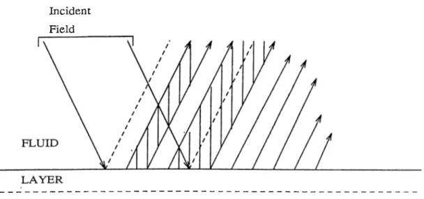
If the layered material is immersed in a liquid medium and insonilied by a bounded acoustic wave, it is seen that the reflected wave is like in Figure 2.2. The important features of the reflected field are the shift and the trailing field in the lateral direction in contrast to the geometrical specuhir reflection [10]. Since the acoustic wave is incident at a critical angle, a particular mode is excited. The mode begins to reradiate back to the liquid medium as soon as it is excited, in other words, some energy of the mode leaks back to the liquid medium causing the mode to be known as a leaky wave mode [11]. The lateral
CHAPTER 2. THEORY
Figure 2.1: The phase velocity of the leaky modes as a function of frequency thickness product for copper layer on steel halfspace.
Incident Field
SUBSTRATE
Figure 2.2: The schematic diagram of nonspecular reflection at a liquid - Iciyered solid material interface. Dashed lines indicate specular reflection, the reflected field is concentrated in the shaded region.
CHAPTER 2. THEORY
Figure 2.3: Magnitude (dotted) and phase (solid) of the reflection coefhcient at water-0.6 mm copper layered aluminum interface as a function of incidence angle at f = 7 MHz.
shift can be related to the Schoch displacement, A 5, and it depends on the material specific space leak rate of the mode. The null region occurs as the result of the interference of the specularly reflected field with the nonspecular component. If the angle of incidence is not a critical angle, the reflected field has no such features, it has only the specular component.
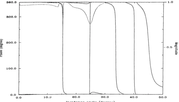
The excitation of the leaky waves reveal themselves in the plane wave re flection coefficient as sharp phase transitions at the critical angles [12]. in Figure 2.3, the magnitude and phase of reflection coefficient at water - copper layered aluminum interface is plotted as a function of incidence angle at a fixed frequency. The sharp transitions in phase indicate mode excitations. One can use this graph to excite leaky modes in the layered material.
2.2
T h e Lam b w ave lens
Leaky wave modes can be excited in a la)^ered solid by acoustic wave insonifica- tion at an appropriate frequency and incidence angle in a liquid medium. This can be achieved easily and efficiently by using a wedge transducer [13], 1)ut it is not suitahle for imaging because of its poor resolution. For high resolution
CHAPTER 2. THEORY
focusing is necessary. A method of focusing surface waves is to use conical waves incident on the solid at a critical angle. Conical waves can be generated by using a conical transducer or refraction or reflection from a suitable surface [14] [15]. The Lamb w'ave lens seen in Figure 2.4 utilizes the refraction api^roach [5].
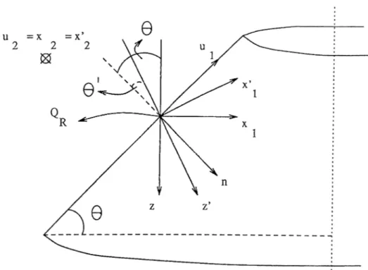
In this geometry, the acoustic waves generated by the transducer are re fracted from the conical recess and form a conical wavefront incident on the layered material. Conical wavefront generation can be shown using the differ ential geometrical approach in [16]. Using the ray fixed coordinate system, the refraction process can be modeled as in Figure 2.5.
In the figure, n is the unit normal vector and Ui and U2 are the principal direction vectors of the conical recess surface at Qr^ Xi and X2 are the prin
cipal direction vectors of the incident wavefront. Since we assuine plane wave incidence, we can freely choose X2 = U2 . The primed quantities denote the corresponding quantities for the refracted ray. Then, using the approach in
CHAPTER 2. THEORY
Figure 2.5; Geometry for refraction at Qn. The plane of incidence is the plane of the paper.
[16], we have the relation,
/c'0'^Q '© ' = k Q ^ Q Q + hC (2.1)
where k, k' are the wave numbers in the leas and liquid medium and Q and Q' are the curvature matrices of the incident and refracted wavefronts in the principal directions, respectively. C is the curvature matrix of the surface at Qf{ and h = k' cos $ — k cos 9\ superscript T denotes the transpose. The matrix 0 is defined as
X l · U i X i · U2 X 2 · U i X 2 · U2
© = (2.2)
with the choice of X2 = we have
© = cos 9 0
0 1
©' = cos 9' 0
0 1 (2,3)
Considering plane wave incidence, i.e. Q = 0 since radii of curvature are infinite and ©''^’ = ©', the curvature matrix of the refracted wavefront can be found as
1
Q' = - © '-l/iC © '- ^
^ h! (2.4)
It is shown in the appendix that for a cone of half angle a — 90 — drawn in Figure 2.6, the surface curvature matrix at Qn is
CHAPTER 2. THEORY i O A C = 0 0 Q —4 sİIг^ 6 (2.5) xq sin 29 _
Then using Eq. 2.4 the curvature matrix of the refracted wavefront is written as
Q' = (cos — Yi cos 9)
0 -4 sin^ eXQsh\29 _ (2.6)
Referring to Figure 2.6, the cone drawn for the refracted wavefront has a'= 90 — (6> — O') and x'q = xqcosO! cos{9 - O'). Also from SnelPs law we have cost?' — -pcosO = sin(t? — 0 ' ) / smO. Substituting these in Eq. 2.6 we get the result as
" 0 0
n —4 sin^(^—
Xq sin 2(0-9')
Q' = (2.7)
Realizing that Q' is the curvature matrix of the lower cone in Figure 2.6 with respect to the principal directions x i ' and X2', we see that the refracted wavefront is conical and has the shape seen in Figure 2.6. As a result we conclude that the Lamb wave lens transforms the incident plane wave to a conical wave with incidence angle 0 - 0 ' and curvature matrix Q'.
CHAPTER 2. THEORY
Fiaclia.1 didtemce
Figure 2.7: Incident and reflected spatial field distributions on the surface of the sample with 0.5 mm copper laj'er on steel substrate.
the angle of the refracting cone and taking Snell’s law into consideration at the lens material-liquid interface. Using the dispersion curves, this angle can be chosen to match a critical angle. If the waves are incident at a critical angle, an evanescent Lamb wave is excited in the material. The Lamb wave lens detects the leaky waves with approximately 30% efficiency. This low efficiency results from the fact that most of the reflected field is blocked by the central part and some of the field leaks bejmnd the lens aperture.
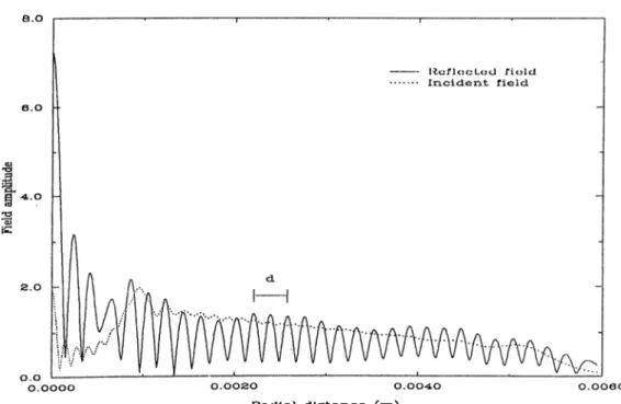
The leaky waves converge in the material and focus at the point where the cone axis intersects the material plane. This focusing can be seen in Figure 2.7 in which the calculated incident and reflected field distributions on the layered material surface are plotted. The calculation is done at a frequency where a Lamb wave mode is excited. The distance between the ripples in the reflected field, d, satisfies the relation d — Xyjj sin where is the wavelength in water at excitation frequency and 6 is the incidence angle. This relation .shows that the reflected field pattern is the result of the interference between the leaky wave components excited from opposite sides of the lens, leaking into the liquid at the same angle 9. If the leaky wave is not excited, the reflected field is nearly same as the incident field and the focusing effect is not seen.
The focused waves then diverge from the focus and leak back to the licpiid at the same critical angle. After refraction from the conical surface, the waves
CHAPTER 2. THEORY 10
Figure 2.8: R{f ) curve at an incidence angle of 35.8 degrees at water- 0.5 mm copper layered steel interface.
are detected by the transducer. To prevent detection of the specularly reflected waves, the distance between the lens and the material, Z, should satisfy the condition Z < { R i / tai: 9 — (i?2 — Ri) tan ^i).
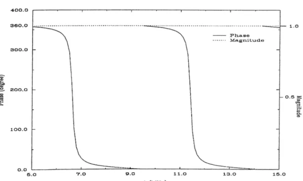
Since the leaky waves are dispersive, the fixed incidence angle of the lens can be made equal to a critical angle of a Lamb wave mode by adjusting the excitation frequency. By choosing the frecpiency properly, the ntodes can l>e excited in a selective manner. In Figure 2.8, the variation of the reflection coefficient at a fixed incidence angle as a function of frequency, R{ f ) curve, is plotted for a copper laj^'ered steel substrate. The phase transitions indicate mode excitations, hence show that desired modes can be excited by adjusting the frequency.
In the design of the Lamb wave lens, some points must be taken into con sideration. The cone angle should be chosen using the dispersion curves of the layered materials of interest. The aperture width must be decided properly by considering the slope of the phase trcinsitions in the reflection coefficient, hence the Schoch displacement. The transducer size and the lens rod length must be chosen to minimize the diffraction loss and the interference from the spurious pulses. The effective width of the conical surface must be large enough to have a narrow angular spectrum around the incidence angle. The effective width can be defined as the portion of the conical surface that is illuminated by the
CHAPTER 2. THEORY 11
transducer at the right incidence angle. If the angular spectrum is wide, i.e. there are wave.s incident at angles difFeri'iit from tlu' desired angle, tin,' excita tion frequencies can deviate from the calculated values. The transducer must have a wide bandwidth in order to have a frequency scan. A matching layer should be deposited on the conical surface to decrease mismatch loss.
2.3
R esp o n se o f th e Lamb w ave lens
The electrical return signal at the transducer terminals can be found by eval uating the voltage integral formula [17]. The formula gives the output voltcvge at the transducer terminals in terms of the scalar wave potential only, in case of longitudinal wave excitation. The scalar potential can be found by using angular spectrum and ray theory techniques. In the following formulae, the superscripts + and - denote the potentials going in the +z and direc tions, respectively and the subscript numbers show the plane of evaluation. Referring to Figure 2.4, following this notation, the spatial scalar potential at the transducer plane, Uj", due to a circular transducer of radius a generciting longitudinal waves, can be written as
^ circ[(a;^ + where circ(r) = 1 r < 1
0 r > 1 (2.8)
The angular spectrum at the same plane, , can be found by Fourier trans formation:
Ui(kx,ky) = F { W } { x , y ) } = i a ‘Ai mc[(ali r)(kl +ki yl ^\
= 2r a M J M . K + k l f l ^ V H k l + kl f l ^\ (2.9) where Ji is the Bessel function of the first kind and and ky are the x and y components of the wavevector, k i, in the lens rod. Since the lens rod has length /, the angular spectrum at 2: = /, ■, can be found as
U^ikx^ky) — jinc[(a/7r)(Â:^ -f kyy^‘^]exp{jk:,l) (2.1 0)
where k. = (kf — k^ — is the component of k i in the -2 direction. The exponential factor, exp(jkzl), takes care of the plane wave propagation in z direction, hence the diffraction. Then the spatial distribution, u j , is found by inverse Fourier transformation:
CHAPTER 2. THEORY 12
To find the field distribution at plane 3, ray theory is used. Referring to Figure 2.9, it is seen that, since the center part is blocked, only the field distribution in the region R\ < (α:^ + < R2, contributes to the field at plane 3. Using ray theory, keeping the amplitude of the rays constant and changing its phase taking care of the ray paths in the lens rod, the field distribution at the conical surface is found. Then the rays are refracted from the surface according to Snell’s Law, the amplitude is scaled by Ar considering
power conservation and the pha,se is changed taking care of the path in the liquid. So, the spatial field distribution at plane 3, Ug , is found approximately as
+ / ^ I { r' /ry^^ARut{r' )exip{j{kidi + k2d2)} Ri < r ' < R2
(^) = \ (2.12)
0 elsewhere
where /[r = (1 + tiin tan(i<i - 02))^^'\ r = (.t'^ + r' = (?· + R2 tan Ox tan(i>i - i*2) ) /(l + tan 0i tan(ili - O2))·, ki sin 0i = ¿2 sin O2, and di = {r' - Ri) tan and ¿2 = {R2 ~ r') tan Oi/ cos(^i - O2). Here ki and k2 are the wavenumbers in the lens rod and the liquid medium, respectively.
To have propagation to the material surface and reflection at the interface, we transform the spatial field distribution, tij, into angular angular spectrum, U^ , as
CHAPTER 2. THEORY 13
Then the reflected angular spectrum at plane 3, , is written as
U ^ { h , k y ) = U^{K,ky)eyi^{j2k^'Z}n{k^lk2,kylk2) (2.14) where = {k^ — kl — kyY^'^ and the exponential factor takes care of the propagation distance 2Z in z direction, since the distance between the lens and the material surface is Z. The reflection process at the interface is included through the multiplication by the reflection coeiflcient, '¡^{kxlk^.kylkY). The output voltage, V, at the transducer terminals can be found in terms of incident and reflected angulcxr spectra at plane 3, by the help of cin integrcil formula derived from reciprocity relations as
y =
Cl 1^28'k‘^ujP
+ 00 /»+00
k z ^ 3 { k x j ky^U^ (^.T) ky'^ d k x clky (2.15)
where Cn is the longitudinal constant of the liquid medium, u> is the angular frequency and P is the incident power at the transducer terminals. Noting that the problem has circular symmetiy, the substitution, k,. = (t^ + can bo made where kr is the radial wavenumber. Then the output voltage, V, as a function of frequency, / , can be written as
d
(2/16)In the foregoing argument using the ray acoustics approximation, zero field is as.sumed out of a certain region in plane 3 ignoring the dilFiciction from the upper and lower edges of the lens. Some error occurs due to this approximation, but since we find the result by integrating the fields, it becomes negligibly small. Also, it should be noted that the frequency response of the transducer is not taken into consideration in the above derivation.
2.4
V{f) C urves
As seen in the previous section, the output voltage of the Lamb wave lens can be expressed as a function of the frequency of operation, lens geometry and the reflection coefficient of the layered material. By recording the output signal of the Lamb wave lens while the frequency of excitation is scanned, one obtains a charcicteristic V{ f ) curve, which shows the excited modes as peaks.
The formation of V{ f ) curve can be easily explained by transforming the velocity dispersion curves in Figure 2.1 to a critical angle versus frequency curves. For this transformation, a fixed thickness is assumed and the relation
CHAPTER 2. THEORY 14
0 .0 0 0 0.00 4
Z ( i n )
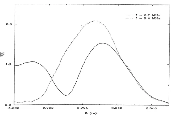
Figure 2.10; The variation of output signal amplitude as a function of lens- sample distance for two different frequency values for the sample in Figure 2.8.
Oc = sin~^{vi/v) is used to transform the velocity to critical angle, where Oc is the critical incidence angle, vi and v are the velocity of sound in the liquid and velocity of the mode, respectively. After this transform, these curves show the variation of critical angle of the modes with frequency. At frequencies where the critical angle ol a leaky mode becomes equal to the fi,xed incidence angle of the Lamb wave lens, the particular mode is excited resulting in nonspecular reflection. In Figure 2.10, the variation of output signal cimplitude as a func tion a function of the distance between the lens and the la3^erecl material is calculated for two frequencies. At / = 6.7 MHz, the critical angle is matched and a leaky mode is excited, so the variation of the field depicted in Figure 2.2 is seen as a peak, a null region and a larger peak. Since the Lamb wave lens is placed close to the material to detect leaky waves, there will be a high outjput signal due to the first peak. At / = 9.4 MHz, the matching condition is not satisfied, no leaky wave is excited and there is onl}^ one peak in V( Z) curve resulting from the specular reflection, hence the output signal is low. Since many modes can be excited at a fixed incidence angle by scanning the frequency, the V( f ) curve takes the form of shifted peaks each corresponding to a different mode, showing the single mode excitiition ability of the Lamb wave lens.
CHAPTER 2. THEORY 15
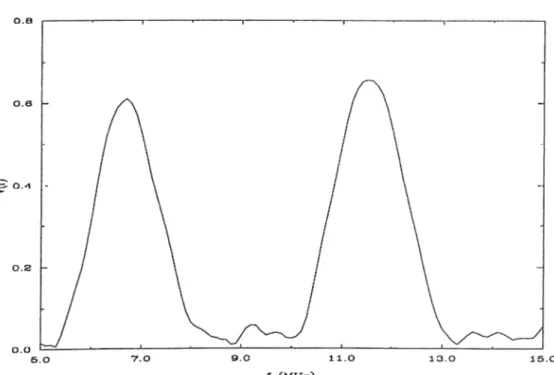
Figure 2.11: The V{ f ) curve of the sample in Figure 2.8.
curve can be observed by referring to the Figures 2.8 and 2.11. The peaks of V{ f ) curve occur at frequencies where phase transitions are observed in the R{ f ) curve, hence the V{ f ) curve directly provides the phase, in other words, critical angle information of the reflection coefficient. In fact, in the frequenc3' range of interest, the magnitude of reflection coefficient is unity and all the information is in the phase which is contained in the V{ f ) curve.
Since any perturbation of elastic and physical parameters of the layered material such as thickness, density, elastic constants and bond quality at the interface changes the reflection coefficient, a corresponding change in V{ f ) is expected. The most drastic change is the shift of the phase transitions in frequency resulting a shift in the peak positions of the V{ f ) peaks. The parameter sensitivity of V{ f ) is investigated by siinulations and the obtained results are presented in Chapter 5.
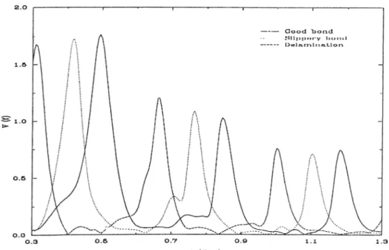
The bond quality at the interface between the layer and substrate is ciiso effective on the V{ f ) curves, since it effects the reflection coefficient through the changes in the boundary conditions. In Figure 2.12, the calculated V{ f ) curves of the aluminum layered silicon sample in water for three bond quality conditions are plotted. In good bond case, perfect bonding at the interface is considered. The case when the layer is in contact with, but slips on the substrate is referred as slippery bond and the delaminated bond corresponds to the condition that the layer and substrate are completely separated by an
CHAPTER 2. THEORY 16
Figure 2.12; Calculated V{ f ) curves for a good bond, slippery bond and de lamination at the interface of 6 /.im aluminum hij'er on silicon substrate. other material. In the delamination case in Figure 2.12, air is assumed to exist between the layer and substrate. All three cases are easily differentiated by observing their effects on the V{ f ) curve showing a unique ability of the Lamb wave lens. In the simulations, a sapphire lens with 0\ = 22° , 0 = 19°, Ri = 42.5 yum and R2 = 250 p.m is used.
C h a p te r 3
S im u lation
In order to compare the theory of the Lamb wave lens with the experiments, a computer program simulating the Lamb wave lens response is developed in C programming language. It mainly consists of calculation of the reflection coefficient and the field propagation and integral calculations involved in the derivation of the V ( /) curve.
3.1
C a lcu la tio n o f th e R eflectio n C oefficient
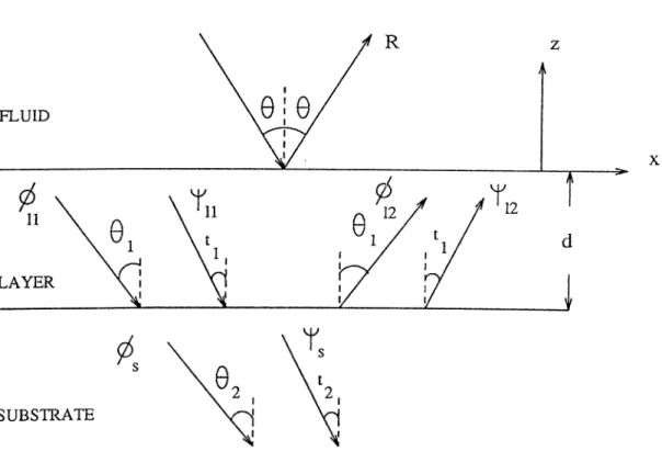
For the reflection coefficient calculation the layered material is modeled as in Figure 3.1. A solid layer of thickness d is assumed on a semi-infinite substrate and this structure is overlaid bj'^ a semi-infinite fluid. Following the notation in [18], we have a scalar potential function $ and a vector potential which correspond to longitudinal and shear wave motion, respectively. Assuming particle motion in x — z plane, we have ^ and With these potential functions, we have the relations
г¿χ = dx dz ( 3 . 1) Ux = 5 $ d'$ dz dx ( 3 .2 ) £)2<i> d-^H d^y\> ^''^^dxdz dx^ dz^ ’ ( 3 .3 ) = 5 2 ^ dxdz (3 .4 ) a rc tlu; t a n g e n t i a l a n d n o r m a l (;o rn i)o n c n ts o f tlu; | ) a r t i d ( ' displacement and and are the tangential and normal stresses, respectively
CHAPTER 3. SIMULATION IS
SUBSTRATE
Figure 3.1: Geometry and coordinate system for the layered material. and A and ¡j, are the Lamé constants related to the longitudinal and shear wave speeds, c/, Cj,, and density, p, as
pcf — \ + 2p, pc] = p (3.5)
Referring to Figure 3.1, assuming that a plane wave of unit cimplitude is in cident on the layered material from the fluid medium at angle 0 we have the wave potentials in the phasor form suppressing harmonic time dependence as
= exp{jkfxs\n0){exp{^—jkfZ cos 0)-{■ Reyiii{jkfZ cos 0)) (3-h)
= exp(;À:/.rsin6'i)((?i/iexp(-jÂ;/2:cosé>i) + (;é;2exp(i/:;’rcos(?i)) (3.7) vj, = exp(;/v/.x-sin Zi)((/>,iexp(-i/c/.rcosii) -f- (/>(2 exp(i/'';2 cos i j ) (3.8)
= exp{jksxsiii02)(f>s^y^p{-jkszcos02) (3.9)
= exç>{jKsXshxt2)i>s^yA>{—ji^sZ costi) (3.10)
where the subscripts / , Iand s denote the media, 1, 2 denote the incident and reflected fields and k and k refer to the longitudinal and shear wave nurnlmrs in corresponding media, respectiveljc
The boundary conditions on the particle displacement and stress are used to obtain a systems of linear equations to solve the unknown potentials [19]. To compare tlie results for different bonding conditions, three separate programs are written employing appropriate boundary conditions for each case.
CHAPTER 3. SIMULATION 19
In good bonding case, the normal component of particle displacement and both tangential and normal stress are continuous at the fluid-hij'er interface with zero tangential stress in the fluid medium yielding the ecjuations
Uzf = u~i, Z,f = Zj;i, Zxi — 0 at z = 0 (3.11) At the layer-substrate interface all the components of the particle disj^lacement and stress are continuous to give the equations
Uxixi — ^^xs^ — ^^zsi Zixi — Zxs^ Zxi — Z;a at z — cl (3.12)
In the case of slippery bonding at the hiyer-substrate interface, the bound ary conditions yielding equations 3.11 remains the same, but since it is as sumed that the layer can slip on the substrate in lateral direction, continuity of tangential displacement is not valid, and the tangential stress is zero at the layer-substrate interface. As a result we have same equations in 3.11 and instead of the equations in 3.12, we have
xizi — '^zs'i Zzi — Zzs Zxi 0, Zxÿ 0 at ^ — cl (3.13)
The delamination case is approximated by assuming that the layer is a solid plate separating two different fluid media. Referring to the Figure 3.1, it corresponds to a fluid substrate. Since we do not have shear potential in the fluid substrate, i.e. number of unknowns is 6. Again we hcive the same equations as in 3.11 and in addition we have the equations
'^zl — '^zs ) Zzl — Zzs4 = 0 at z = —d (3.14) The equations can be written in terms of the unknown potentials by substi tuting the results of equations 3.6 through 3.10 in the equations 3.1 through 3.4. Since we have equal number of equations and unknowns, the reflection coefficient, R, in equation 3.6 can be found in each case of bonding. The de veloped programs evaluate the equations and solve the system of equations for R using Cramer’s rule. The results are in good agreement with the published ones [20] [21].
CHAPTER 3. SIMULATION 20
3.2
C a lcu la tio n o f V(f) C urves
For the calculation of the V{ f ) curves theoretically, the steps exi)la.ined in the section 2.3 arc implemented b}' a program. Since the problem involves many transformations back and forth between spatial and angular domains, an efficient transformation algorithm should be used.
Since the problem has circular symmetry, the Fourier transform becomes the Hankel transform in cylindrical coordinates. An efficient method called Quasi Fast Hankel Transform (QFHT) [22] is used for the implementation of Hankel transform. A pair of Hankel transform of order 0 is defined as
poo g{p) = 2TT / rf{r)Jo{2TTpr)dr (3.15) Jo poo f {r) = 2tt pg{p)Jo{27cpr)dp Jo
For QFHT, first a Gardner Transform variable change is performed
= roexp(ax), p = poexp(ay) (3.16)
where ?’o, Po and a are constants to be determined considering some relations to avoid aliasing. With this variable change and defining new functions as
f {x) = ?’/(?’)=: roexp(a.T)/(roexp(aa;)) g{y) = p/(/>) = Poexp(ay)y(poexp(cvy))
j {x A y ) = 2Traropo exp(.r + 7/).7o(27raro/9o exp(.T + y)) the Hankel transform integrals in Eq. 3.15 become
(3.17) y { y ) = / f {x) j {x + y)dx J— oo
/
00 9{y)i{x + y)dy •OO (3.18)It is observed that the transform integrals are converted into cross-correlation integrals, which can be efficiently evaluated by Fast Fourier Transform (FFT) methods. To apply FFT methods, the functions in Eq. 3.18 are converted to discrete sequences of length N ^ then a discrete approximation to the Hankel transform integrals is written as
N - \
y VA = 5 3 f [ n] j [ n + m] (3.19)
n=0 N - 1
CHAPTER 3. SIMULATION 21
To have correct results, the Л^-point sequences are extended into 2iV-point se quences by padding with zeros from m, n = Л'' to 2Л^ — 1. Then the summations in Eq. 3.19 become 27V-point circular convolutions. The criteria for choosing the parameters 7’o, po and a, considering alicising, becomes
N = K2^bln{Ki/3b), ae xp { a N) = Ki/1<2, vopo = {К2/1<1)а (3.20) where /3 is the highest spatial frequency and b is the largest radial distiince. We have the relations го = If Ki j S and Ар.л/ = 1/ / \ 2^, so the condition A'l, K2 > 2 should be satisfied to avoid aliasing. Once N, Ki and K2 are determined, the other parameters can be found using the relations in Eq. 3.20. Using QFHT, for each Hankel transform, 2Nlog2{lN) complex multiplications and additions are performed, whereas N"^ complex multiplications and additions are required for direct evaluation of the integrals by trapezoid approximation with the same accuracy.
N is chosen ¿vs 4090 lor the cvilcuhvlions, and for evich lens with dill’erent frequency range and dimensions, the other parameters are found satisfying the required conditions. The error resulting from the discrete approximation in Eq. 3.19 is calculated and it is seen to be negligibly smcill. For Ccvch frequency Vcilue, 3 QFHT’s are performed and the field propagation is included by complex multiplications.
In V{J) calculations, the acoustic attenuation in the fluid and the effect of anisotropic lens rod material on diffraction loss are ¿ilso considered for cor rect simulation. The acoustic attenuation in fluid is included in two pcvrts. First, referring to Figure 2.4, each I'ciy reaching phvne 3 after refrciction from the conical recess, is attenuated depending on the length of its path in the fluid. Then, after finding the angular spectrum at plane 3, each j^lane wave component is attenuated considering the propagation between the lens ¿vnd the material surface. The effect of the anisotropic lens rod material on diffraction loss is included by calculating the equivalent diffraction length of the lens rod, using the relation /' = /(1 — 26), where I is the physical length of the lens rod and 6 is the anisotropy f¿гctor [23].
After finding the field distributions at material surface, the voltcige integrcil is evalucvted by trcipezoid ¿vpproxirnation. Tn this evaluation, ¿vt every sampling point, the reflection coefficient at the corresponding incidence angle is calcu lated and multiplied with the field distributions. The re,suit is then normalized by the proper constants to give the final voltage value.
C h a p te r 4
E x p e r im e n t a tio n
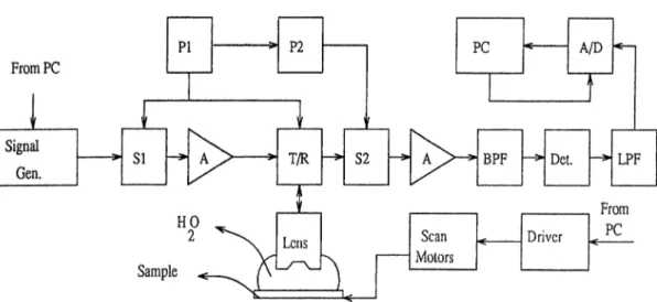
An experimental setup is implenaented and some specially prepared layered samples are used to test the theory of the Lamb wave lens and its ability to characterize and imcige the layered matericils. The functional diagram of the setup is given in Figure 4.1. The setup mainly consists of the Lamb wave lens, electronics to excite the lens properly, scanning system for imaging and a. PC for data acquisition and control.
4.1
T h e Lens
A Lamb wave lens is designed and fabricated for experimental purposes. The lens rod is made of aluminum. Referring to fig 2.4, its length, /, is 5.9 cm. The conical recess has an upper radius, i?x=3.1 mm and a lower radius, i?2= 5.95 mm. The angle of the cone is chosen to be as 0i = 45.5° resulting conical waves in cident to the layered material with an incidence angle, 6 = 35.8° from water after refraction from aluminum-water interface. The center part is blocked b)^ acoustic absorbant to prevent direct reflection from this region.
An air-backed PZT-511 piezoelectric cercunic transducer is used for acoustic wave generation. It has a radius, a=8.5 mm and it is bonded to the lens rod by phenyl salicylate. The transducer has a resonance frequency of 7 MHz with a 3 dB bandwith of 3.4 MHz, limiting the useful band of the setup to 5-9 MHz. With this bandwidth, at most two leaky modes can be excited in the prepared samples with layer thickness in the range 0.4-0.7 mm to obtain a V( f ) curve, since at most critical angles of two modes can be matched to the angle of the lens in this frequency range.
CHAPTER 4. EXPERIMENTATION 23
Figure 4.1: Functional block diagram of the experimental setup.
4.2
E lectro n ic S etu p
The electronic system is operated in the 5-9 MHz frequency band due to the limitation imposed by the transducer, although the com|)onents have a. larger band with. Referring to Figure 4.1, the sine wave of desired frequency generated by the computer controlled signal generator is time gated by the switch Si, which is in turn controlled by the pulser PI. The sine burst is amplified and sent to the transducer through the T /R switch, which is also controlled by PI. The width of the pulse generated by PI should be at least 4-5 cycles long to resemble continuous wave excitation and reduce the band of the signal, but it should be shoii, enough to avoid ¡nterferc'iicc. 800 us is louiid to be a pro]>c;r pulse width for PI. The repetition rate should be high to increase the signal to noise ratio but it should be low enough such that the transducer response will decay in one period. A compromise is found at 800 tiz.
The return signal is passed from T /R switch to switch Si, controlled by pulser P2, which generates a pulse with an adjustable width and delay with respect to PI. The delay between P I and P 2 is adjusted considering the propagation time of the acoustic waves in the lens, liquid and the material to detect only the desired signal reflected from the sample. The signal is then amplified and passed through a 5-10 MHz band pass filter for noise reduction. A negative detector is used to extract the envelope of the signal. The detector output is passed through a low pass filter to get its dc part and amplified before A/D conversion controlled by the computer. For point V{ f ) measurements, the output of the band pass filter is recorded from the scope while changing the frequency.
CHAPTER 4. EyXPERmENTy\TION 24
4.3
Im agin g S etu p
The return signal of the Lamb wave lens can also be used for imaging. If the sample under test is scanned mechanically, while recording the amplitude of return signal at a fixed frequency at every pixel, an amplitude image (AI) of the sample can be obtained. High contrast APs, showing the spatial variation of material parameters, bond quality and subsurface defects in the sample, can be recorded if the frequency is properl}^ adjusted.
In our imaging setup, the sample is placed in a water-filled tcink mounted on a surface which can be mechanically scanned. Two identical stepper motors are used to move the sample in the X — Y plane in raster fashion. The motors have maximum speed of 250 steps/sec. with a step size of 10 /iin. They are driven by a driver unit controlled by the computer (Figure 4.1). During the imaging process, the computer moves the sample and at every imaging point, it performs an A/D conversion, then stores the pixel value in the memory. The PASCAL program is written to perform the above operations. W ith the present setup, AI of a 2 cnE area is taken in nearly 15 minutes with 200 points in each direction. The mechanical speed is the limiting factor, with faster motors this duration can be reduced.
As pointed out in section 2.4, the shift in the peak frequency of a par ticular mode is the most significant result in V{f ) , when a change occurs in the parameters of the material or bond quality at the interface. So, a peak frequency image (PFI), formed by mapping the peak frequency of a particular mode in the V{ f ) curve, can directly provide information about the related local properties of the layered material.
For PFI, at every imaging point the frequency is scanned in a range, i.e. V( f ) is recorded, and the peak frequency is found by detecting and comparing the return signal at every frequency step. Then the peak frequency value is stored as data of that pixel. A computer program, which scans both the sample mechanically and the frequency electronically synchronously with data acquisition is written. The frequency scan is done by controlling the signal generator using IEEE 488 Standard. For this purpose, an IEEE 488 interface card is installed in the PC and operated by a program in BASIC. A PFI of a 2 crrP area is taken in the order of hours with 0.1 MHz frequency steps and 0.1 mm step size in both directions. The speed is limited by mechanical reasons and the scan speed of the signal generator.
CHAPTER 4. EXPERIMENTATION 25
4.4
T h e S am p les
In order to investigate the characterization and imaging ability of tlie Lamb wave lens, some layered materials are specially prepared as samples. Con sidering the geometry and frequency band of the fabricated lens, some layer- substrate pairs are found to be suitable for investigation by the help of the simulation program. Among them, copper layer on steel substrate is seen to be feasible to prepare.
Copper layer is deposited onto steel by electroplating. It is known that to have a strong bond between the deposited layer and steel substrate, the substrate should be processed in copper cyanide solution prior to the regular plating process in copper sulphate solution [24]. This fact is used to produce well defined regions of poor bond at the interface. After cleaning the surface, the areas at which poor bond is desired are masked and the substrate is plated in copper cyanide solution. Then, the mask is removed and the plating is continued in copper sulphate solution. The samples are plated to a thickness of 0.7 mm and then surface ground to required levels. Since the layer thickness should be in the order of wavelengths, the layer thickness was kept in the 0.4 - 0.65 mm range. The samples show no optical indication of different bond regions.
C hapter 5
R esu lts
In this chapter, simulated and experimental V{ f ) curves are presented and compared. The amplitude and peak frequency images of a sample are pre sented.
5.1
V{f) R esu lts
The theory of the Lamb wave lens is checked by comparing the theoretical V{ f ) curves computed by the simulation program with the experimental V{ f ) curves measured on the prepared samples by the setup explained in Gha.pter 4. Especially the eifect of bond quality on V{f ) is investigated. In the compar isons, both the experimental and simulation results are normalized considering the frequency response of the transducer. In Figure 5.1, the calculated and measured V{ f ) curves of a sample with 0.6 mm copper layer on steel substrate are compared. In simulations three bonding conditions are considered. The V{ f ) measurements are done at two spots. One is at a good bond region and the other is at a point where a poor bond is induced. The coinparisoii sliows that the poor bond is a slippery bond. In Figure 5.2, a similar comparison is made for another sample with 0.5 mm copper layer. In this case, it is seen that the poor bond is a delamination with air separating the la3^er and the substrate. In both cases good agreement is observed between the computed and measured curves.
The parameter sensitivity of V{f ) is investigated by simuUrtions performed on an 6 /iin aluinimim la\'ered silicon substrafe sample. As seen in Figure 5.3, the V{ f ) is very sensitive to changes in the density, p, and the shear constant, C44. In the siinuUrtions, a sapphire lens operating in 0.8-1.3 GHz frequency
CHAPTERS. RESULTS
f ( M H z )
Figure 5.1: Calculated and measured V( f ) curves for a good bond and slippery bond. The sample is 0.6 mm copper layered steel substrate.
band with Ѳ = 19°, Ri = 45 /.im, R2 = 300 is used. The percent shift in the peak frequency of V{ f ) curve of a particular mode as function of percent changes in the shear constant, C44 , and the density, p, of the laj'^er material is plotted in Figure 5.4. It is seen that for small perturbations, the relation is almost linear. It i.s · Iso observed that the cil'cct of Cu of the layer a n d the parameters of the substrate have negligible effect on V( f ) peaks. The shear wave velocity of the layer is the most effective parameter on V[ f ) curves.
In all the layered materials considered above, the layer has softer acous tic properties than the substrate. This case is referred in the literature as “Zoaded” substrate. To show the application of V( f ) technique to the oppo site case, which is called ‘^stiffe n ed ” substrate, simulations are also done on chromium layered steel substrate. This kind of layered materials support only the Raylcigh-like mode [20]. In Figure 5.5, the Ccilculated V{f ) curves of 40 pm chromium layered steel are plotted for good bond, slippery bond and delamina tion cases. The simulations are done assuming a lens made of glass operating in 20-40 MHz frequency band, with Ѳ — 31.8° , Ri = 0.98 mm, and R2 — 2.64 mm. A peak is observed in the frequency range of interest for slippery- bond and delamination, in contrast to the low signal level for good bond case, showing that the Lamb wave lens can also be used to differentiate bond quality in stiffened substrates.
CHAPTER 5. RESULTS 28
f ( M H z )
Figure 5.2: Calculated and measured V{f ) curves for a good bond and a delaniination. The sample is 0.5 mm copper layered steel substrate.
5.2
Im ages
The spectral shape of tlic V{f ) curve is determined by the reflection coefficient of the layered material at that point. Since the reflection coefficient is highly dependent on the bond quality at the layer-substrate interface, V{ f ) directly provides bond quality information. Part of this information can be exploited b}'^ obtaining amplitude images as explained in section 4.3. If the frequency of excitation is chosen such that the amplitude difference between different types of bond is maximized, the resulting image will indicate the regions of different bond quality successfull}c For the sample in Figure 5.1, 7.9 MHz was chosen as the frequency of excitation for amplitude imaging, providing maximum ampli tude difference between slippery and good bond regions. Figure 5.6 shows the amplitude image of a 2 cm by 2 cm region of the sample described in Figure 5.1. The induced slippery region is a 1 cm by 1 cm square, and it is clearly identified. It should be noted that the regions with different bond quality are not differcnt^.blp optically.
As seen ^ ■ Figure 5.1, the frequenc}'^ of the peak in V{ f ) due to a particular mode shifts irom 9.7 MHz in case of good bond, to 8.1 MHz in the case of slippery bonding at the interface. Hence a peak frequency image fPFI) can be formed as explained in section 4.3 to differentiate the bond quality. For
CHAPTERS. RESULTS 29
f ( G H z )
Figure 5.3: Calculated V{ f ) curves for unperturbed, and perturbed layer pa rameters in case of good bond. The density, p, and shear constant, C44, of the layer ai'e increased 5 %.
the sample in Figure 5.1, at every imaging point, the local peak frequency around 8 MHz is found and a PFI is formed by plotting the peak frequency as a function of position. The obtained PFI of the same region in Figure 5.6 is shown in Figure 5.7. The regions with high intensity indicate higher peak frequencies, i.e. the regions with good bond at the interface, and the dark region caused by lower peak frequencies, shows the induced poor bond. Again the square shaped poor bond region is identified and the peak frequenc}^ is constant in that region.
The axial resolution of the images is equal to the layer thickness since the Lamb wave modes propagate predominantly in the layer. The lateral resolution is not very easy to define since any perturbation in the region that is insonified by the lens disturbs the return signal, but the effect of the focal region is the most significant. It should be noted that no sign of these bond differences at the interface is visible optically on the surface of the samples.
CHAPTERS. RESULTS 30
6 . 0
Cla«LXigo i n c-44 (%)
1.0 T-l.O
Ch&nse In r h o (%)
Figure 5.4: Calculated percentage shift in V( f ) as a function of percentage changes in layer p and C44.
f (MFIss)
Figure 5.5: Calculated V{ f ) curves for good bond, slippery bond and delami nation for 40 p m chromium layer on steel substrate.
CHAPTERS. RESULTS 31
Figure 5.6: Amplitude image of the sample with 0.6 mm Cu layer on steel at 7.9 MHz.
^ \''i\ --iv. V .X sssXA:j$X\ V i'" X
C hapter 6
C on clu sion
The Lamb wave lens can be used as a lens of acoustic microscopes for quantita tive characterization and imaging of layered materials. The unique V{ f ) curve of the layered material, obtained by a simple frequency scan, emerges as a new characterization method providing plenty of information about the elastic and physical parameters of the material and the bond qualit}'· at the interface. The good agreement seen between the experimental and theoretical results show that the technique can be used to make sensitive parameter measurements.
In the V{ f ) measurements, the main mechanical accuracy requirement is the alignment of the samples with the lens to have right angle for detection of reflected waves. The Lamb wave lens does not have a critical focusing problem of the spherical lens, as long as it does not receive specular reflections, the distance to the material surface does not alter the output signal significantly. As a system requirement, a system using the Lamb wave lens should be able to scan the operation frequency to excite different modes because of the fixed incidence angle. Also, to investigate different layered materials. Lamb wave lenses with different incidence angles may be required.
The Lamb wave lens can easily identify bonding problems in layered materi als. It can differentiate the nature of some bonding problems at the interfaces, which is by other means very difficult. Images of such interfaces can either be made in the form of an amplitude image or a PFI. For amplitude imaging, the irequency should be properly adjusted so as to have maximum contrast. As compared to amplitude images, PFI images contain more information and are safer to interpret.
The Lamb wave lens, which becomes a powerful tool for layered material
CHAPTER 6. CONCUJSTON 33
characterization and imaging, seems to have a promising future with applica tions to multilayered materials, anisotropy and attenuation measurements.
A p p en d ix A
C alcu lation o f th e curvature m atrix o f a cone
For a curved surface ^ = /(a;, xj) with 2-axis normal to the surface at the point P where x — y = z = Q. the curvature matrix of the surface at P in the directions of x and y axes is defined as
C = j x x f x y
f x y f y y
where fxx = f ¡dx^ etc. are evaluated at x = y = 0.
(A.l)
Let us consider a cone in rectangular coordinates as in Figure A.l with half angle a. Then the formula of the cone can be written as
x^ = cot'^ a[z^ -h y^) (A.2)
where cota = c/a. Suppose that we want to find the curvature matrix at an arbitrary point P as shown in Figure A.l. To have 2-axis normal to the surlace of the cone the x and 2 axes are rotated by a- degrees counterclockwise resulting in the primed coordinates as
X — z' sin a -\- x' cos fv, z — z' cos rv — x' sin o, y — y' ••0 Eq. A.2, after some manipulations, can be written in primed coordinates as
cos^ a . z'^ — x'z'iaxi2a -f y'^i---) = 0
cos 2a A.4)
To have x" = y” = 2" = 0 at point Pq, the .x'-axis is shifted by an iimount xq to yield new coordinates
x ” - x' - xo, z" = 2', y" = y' Then Eip A.4 becomes
pn _ ta n 2 a -H y " \ ^ ^ ^ ) = 0
cos 2 a ‘
(A.5)
(A.6) 34
APPENDIX A. CALCULATION OF THE CURVATURE MATRIX OF A CONE35
Figure A.l: Geometry and the coordinate system of the cone.
To have the equation of the surface in the form z" = f{x",y")·, z ” is solved from Eq. A.6. The roots of Eq. A.6 can be found as
+ ^’o) tan 2a q: \/A } (A.7)
where A = (x" + rco)^tan^2o; — iy " ‘^[cos^ a j cos2a). The root with positive sign is taken to have a convex surface.
To find the curvature matrix, the derivatives, f x " x " , f x " y " and fynyn are
found and evaluated at x" = y" = 2" = 0 resulting Jr"r" = = 0
4 COS^ Q'
J y " y " =
---Xq sm 2a
Thus, the curvature matrix, C, of the cone cit point P is found as
C = (A.8) (A.9) ' 0 0 R^n1 0 0 x o s i n 2 a _4 cos^ Oi 0 1 Ry// (A.IO)
where Rxh and Ryu are the radii of curvature in the directions of the x" and
A p p en d ix B
M aterial C on stan ts U sed in S im u lation s
In this appendix, the longitudinal acoustic wave velocity, Vi, shear acoustic wave velocity. Id,, and density, p, of the materials used in the simulations are tabulated.
Material Vi{mlsec) Vs {mlsec) piglcm^)
Air 344 1.24x10⁻³ Aluminum 6420 3040 2.7 Chromium 6650 4030 7.0 Copper 5010 2270 8.93 Glass (Pyrex) 5640 3280 2.24 Sapphire 11100 6040 3.99 Silicon 11000 6250 3.27 Steel 5900 3200 7.9 Water 1509 1.0 36
R eferen ces
[1] R. B. Thompson and D. O. Thompson, “Ultrasonics in nondestructive cv<i.lnation,” Proc. ¡¡'¡PI'J, vol. 73, pp. ITKi-lThD, December 1985.
[2] C. F. Quate, A. Atalar and H. K. Wickramasinge, “Acoustic microscopy with mechanical scanning-a review,” Proc. IEEE, vol. 67, pp. 1092-1114, 1979.
[3] A. Atalar, “An angular spectrum approach to contrast in reflection acous tic microscopy,” J. Appl. Phys., vol. 49, pp. 5130-5139, 1978.
[4] K. K. Liang, G. S. Kino and B. T. Khuri-Yakub, “Material characteri zation by inversion of V(Z),” IEEE Trans. Sonics Ultrason., vol. 32, pp. 213-224, 1985.
[5] A. Atalar and H.Koymen, “A high efficiency Lamb wave lens tor subsurface imaging,” in Proc. IEEE 1989 Ultrasonics Symposium, pp. 813-816, 1989. [6] A. Atalar, 11. Koymen and L. Dcgertekin, “Characterization of layered
materials by the Lamb wave lens,” in Proc. IEEE 1990 Ultrasonics Sym posium, pp. 359-363, 1990.
[7] A. Atalar, L. Degertekin and H. Koymen, “Acoustic parameter mapping of layered materials using a Lamb wave lens,” Acoustical Imaging, vol. 19, 1991.
[8] G. W. Adler and E. L. Farnell, “Elastic wave propagation in thin la3?ers,” in Physical Acoustics, W. P. Mason and R. N.Thurston, eds., vol. 9, pp. 35-127, Academic, 1972.
[9] D. E. Chimenti, A. H. Nayfeh, “Leaky Lamb waves in fibrious composite laminates,” J. Appl. Phys., vol. 58, pp. 4531-4538.
[10] H. L. Bertoni and T. Tamir, “Unified theory of Rayleigh-angle phenomena for acoustic beams at liquid-solid interfaces,” Appl. Phys., vol. 2, pp. 157- 172, 1973.