c
⃝ T¨UB˙ITAK
doi:10.3906/elk-1409-19 h t t p : / / j o u r n a l s . t u b i t a k . g o v . t r / e l e k t r i k /
Research Article
Design and walking pattern generation of a biped robot
Tolga OLCAY1,2,∗, Ahmet ¨OZKURT3
1Department of Mechatronics Engineering, The Graduate School of Natural and Applied Sciences,
Dokuz Eyl¨ul University, ˙Izmir, Turkey
2
Department of Mechatronics, ˙Izmir Vocational School, Dokuz Eyl¨ul University, ˙Izmir, Turkey
3
Department of Electrical and Electronics Engineering, Faculty of Engineering, Dokuz Eyl¨ul University, ˙Izmir, Turkey
Received: 02.09.2014 • Accepted/Published Online: 20.02.2016 • Final Version: 10.04.2017
Abstract: This paper presents the design of a biped robot, the walking trajectory generation method, and
experi-mental results about biped walking. Walking trajectory generation is one of the deterministic factors in walking robot applications. Different approaches for stable walking trajectory are worked on in robotic research. The linear inverted pendulum model (LIPM) is an effective method used with the zero moment point (ZMP) criteria. Biped robot trunk and feet moving patterns are generated depending on these fundamental methods. In this study, generated trajectories were tested by a 12 degree of freedom (DOF) biped robot RUBI built at Dokuz Eyl¨ul University. In the experimental work, the joint angles obtained by using inverse kinematics from the generated trajectories were implemented on the robot. The results showed that even with a simple control system implementation of generated trajectories is very promising in terms of stability and reducing complexity.
Key words: Walking trajectory generation, zero moment point, inverted pendulum, biped robot
1. Introduction
In recent years, there has been growing interest and projects on walking biped robots [1–4]. Biped robots inspired by human motions have higher mobility than other robots do in various environments. Although biped robots have many advantages compared to other types of robots, the control of biped robots is a challenging problem that is unbalanced, nonlinear, dynamically time variant [5,6].
One of the main problems is continuously and dynamically balanced walking pattern generation. There are many methods and techniques to overcome that requirement [7,8].
The linear inverted pendulum model (LIPM) is one of the solution techniques [9–12]. The biped robot is treated as a simple inverted pendulum problem. When the robot trunk starts to fall while walking, the supporting leg prevents it from falling.
Another popular approach to the dynamic stability method for generating a walking pattern is the zero moment point (ZMP) criterion [4,13]. The ZMP is defined as the point on the ground where the total moments of the active forces equal zero. If the ZMP is within the convex hull of all contact points between the feet and the ground, dynamically stable walking motion can be achieved.
This paper presents the design of a biped robot RUBI and its walking pattern generation using LIPM and ∗Correspondence: [email protected]
ZMP techniques together. Moreover, walking test results and their analysis are discussed. As a contribution to this subject, in this study, a walking pattern generation method for small biped robot equipped with simple sensor structures and having relatively low complexity was realized.
After the brief introduction about the construction of the biped robot RUBI in Section 2, details about the suggested walking pattern generation method are given in Section 3, control systems are summarized in Section 4, and experimental results and the conclusion are given in Section 5 and Section 6, respectively.
2. Biped robot RUBI
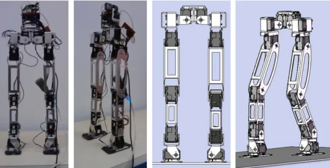
The biped robot RUBI is designed 1:2.3 the proportion of the human lower body. The biped robot and its CAD model are shown in Figure 1.
Figure 1. Biped robot RUBI and its CAD model.
RUBI was developed according to human-like shape with a trunk, human-like movements, compact size and light weight, kinematically simple structure, and low power design philosophy. Therefore, the locomotion system of the bipedal robot was limited to 12 degrees of freedom (DOF). The DOF of the robot are summarized in Table 1.
Table 1. Degrees of freedom of RUBI.
Joint Direction Degrees of freedom
Hip x, y, z 3 d.o.f. × 2 = 6 d.o.f.
Knee y 1 d.o.f. × 2 = 2 d.o.f.
Ankle x.y 2 d.o.f. × 2 = 4 d.o.f.
12 d.o.f.
Robot joints are driven with various sensors embedded Dynamixel smart robot servos. RUBI is also equipped with foot force sensors and an inertial measurement unit. The physical dimensions of RUBI are shown in Table 2.
Table 2. Physical dimensions of RUBI.
Height 481 mm
Width 190 mm
Depth 68 mm
Length of thigh (the hip to the knee) 232 mm Length of shin (the knee to the ankle) 141 mm Length of ankle (the ankle to the foot) 72 mm
3. Walking pattern generation
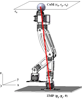
In this work, the linear inverted pendulum model (LIPM) and fixed zero moment point (ZMP) are used to generate the walking pattern. The method in this study is based on finding the center of mass (CoM) position with ZMP reference given. This technique assumes that the mass of legs should be much less than that of the biped robot trunk and all mass concentrated in one point at the biped CoM. It is also assumed that the motion of CoM moves in fixed height surface. This model is shown in Figure 2.
Figure 2. LIPM model of biped robot.
In this figure, the ZMP is described by a point on the supporting foot (px, py, 0) and the position CoM
is described by (cx, cy, cz) , where g is the gravity constant, the fixed height of CoM cz = z and m = mass of
biped robot.
The equations of ZMP with CoM positions can be written from gravity torque and acceleration torque balance.
px=cx−
cz
py=cy−
cz
gc¨y (2)
For robot stability, ZMP should be on the supporting foot area while the swing foot is moving. When both feet are on the ground in the double support phase, ZMP moves from one foot to the other. This action is repeated in walking. Therefore, the reference ZMP trajectory can be used for generating the walking pattern. Choi et al. [12] worked on an indirect ZMP controller with this idea. It is assumed that the reference ZMP trajectories are shown in Figures 3 and 4. This assumption says that ZMP is always in the middle of the supporting foot and changes quickly to the other foot during walking. Therefore, the equations of reference CoM trajectory cx
and cy are 0 0.5 1 1.5 2 2.5 3 −100 −50 0 50 100 150 200 250 300 350
400 ZMP and CoM Trajectory along X−axis
Time (s) ZMP X(t ) and CoM X(t) (mm) ← Reference ZMP Fourier appx. ZMP → ← Reference CoM 0 0.5 1 1.5 2 2.5 3 −100 −80 −60 −40 −20 0 20 40 60 80
100 ZMP and CoM Trajectory along Y−axis
Time (s)
ZMP Y(t
) and CoM Y(t) (mm)
← Reference ZMP
← Fourier appx. ZMP
← Reference CoM
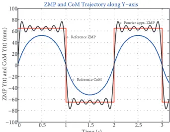
Figure 3. Reference ZMP px, Fourier approximation reference ZMP prefx , and reference CoM trajectories crefx are when n = 12.
Figure 4. Reference ZMP py, Fourier approximation reference ZMP prefy , and reference CoM trajectories crefy are when n = 12. cx(t) = B ∑∞ k=1[1− cosh wn(t− kT )] u (t − kT ) (3) cy(t) = A [1− cosh wn(t)] +2A ∑∞ k=1(−1) k [1− cosh wn(t− kT )] u (t − kT ), (4)
where T is step period, A is the distance between the two feet centers in the y direction, B is the step distance in the x direction, and w2
n = g/cz. Eqs. (3) and (4) cannot be used because of the unbounded function cosh.
Moreover they are very sensitive to the change in wn. Therefore, one of the approximate solutions with Fourier
series [12] is suggested in biped walking robots. In this method, reference ZMP pref
x and prefy are expressed as
the odd functions with period T, and reference CoM trajectories crefx and crefy are assumed as Fourier series.
After finding the Fourier coefficients, cref
x and crefy are expressed as
crefx (t) = B T0 ( t−T0 2 ) +∑∞ n=1 BT2 0w2n(1 + cos nπ) nπ (T2 0w2n+ n2π2) sinnπt T0 (5) crefy (t) =∑∞ n=1 2AT2 0w2n(1− cos nπ) nπ (T2 0wn2+ n2π2) sinnπt T0 (6)
Reference ZMP, Fourier approximation reference ZMP, and reference CoM trajectories are shown in Figures 3 and 4.
Figures 3 and 4 are plotted with A = 65 mm, B = 110 mm, T = 1 s, and w2
n = 21.36 (cz = 459 mm and
g = 9.81 m/s). Although these ZMP references have a small double support phase and the Gibbs phenomenon, approximate solutions of CoM references are suitable for biped robot applications.
The swing foot trajectories are easily generated by function-based spline [13,14]. Generally, simple expressed curves are used with some assumptions. On the sagittal plane, Huang et al. [14] expressed foot trajectories by a vector Xa = [xa(t), za(t), θa(t)]T, where xa(t), za(t) are the coordinates of the ankle
position, and θa(t) is the angle of the foot.
The parameters for swing foot calculations are given as follows. The period for one walking step is Tc.
Td is the interval of the double-support phase. Lao and Hao are the position of the highest point of the swing
foot ankle, which is important if there are obstacles in environments, and Tm is the time that the swing foot
reaches the highest position. Ds is the length of one step, lan is the height of the foot, lab is the length from
the ankle joint to the heel, and laf is the length from the ankle joint to the toe.
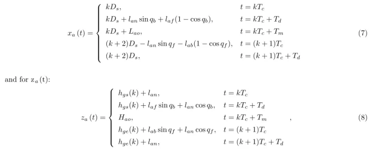
Thus, the above constrains are obtained for xa(t):
xa(t) = kDs, t = kTc kDs+ lansin qb+ laf(1− cos qb), t = kTc+ Td kDs+ Lao, t = kTc+ Tm (k + 2)Ds− lansin qf− lab(1− cos qf), t = (k + 1)Tc (k + 2)Ds, t = (k + 1)Tc+ Td (7) and for za(t): za(t) = hgs(k) + lan, t = kTc hgs(k) + lafsin qb+ lancos qb, t = kTc+ Td Hao, t = kTc+ Tm hge(k) + labsin qf+ lancos qf, t = (k + 1)Tc hge(k) + lan, t = (k + 1)Tc+ Td , (8)
where qgs(k) and qge(k) are the angles of the ground surface, and hgs(k) and hge(k) are the heights of the
ground surface under the support foot. qgs(k) = qge(k) = 0 and hgs(k) = hge(k) = 0, if the support foot is
on level ground. In other words, the robot moves on the flat surface. In this work, we assume that the swing foot is moving parallel to the ground. Thus the angle of the foot is θa(t) = 0 when walking.
To obtain a smooth trajectory, first and second derivatives of xa(t) and za(t) should be continuous at
all breakpoints. When third-order interpolation is used, the second derivatives xa(t) and za(t) are always
continuous. Therefore, using third-order interpolation is the best way to find xa(t) and za(t) [14].
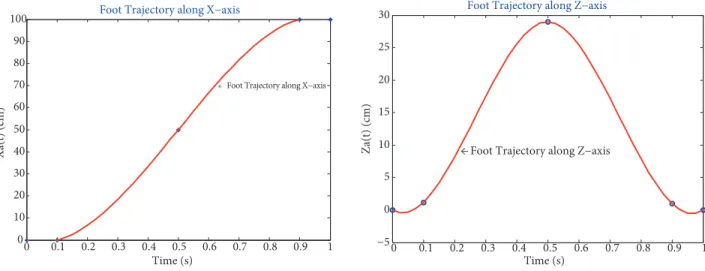
For one simple step, the step length was 50 mm/step with the step period of 1 s/step and the position and time of the highest point of the swing foot ankle were Lao = 50 mm, Hao = 100 mm, Tm = 0.5 s, and Td
= 0.1 s. With these parameters, foot and hip trajectory were achieved using third-order interpolation.
Figure 5 shows the foot trajectory along the x-axis according to Eq. (7) and Figure 6 shows the foot trajectory along the z-axis according to Eq. (8).
0 0.1 0.2 0.3 0.4 0.5 0.6 0.7 0.8 0.9 1 0 10 20 30 40 50 60 70 80 90
100 Foot Trajectory along X−axis
Time (s)
Xa(t
) (cm)
← Foot Trajectory along X−axis
0 0.1 0.2 0.3 0.4 0.5 0.6 0.7 0.8 0.9 1 −5 0 5 10 15 20 25
30 Foot Trajectory along Z−axis
Time (s)
Za(t) (cm) ← Foot Trajectory along Z−axis
Figure 5. Foot trajectory along x-axis. Figure 6. Foot trajectory along z-axis.
4. Control systems
The joint angles of the biped robot are obtained with inverse kinematics from CoM and the swing foot trajectory. Each smart joint actuator, which has its own PI controller, is driven independently. An embedded PI position controller corrects joint position in 0.3◦ degree error. In addition, balanced foot contact controls are implemented with force sensors. That is a simple balancing feet ground force application. Currently, except for these controllers, the global control system is an open-loop system.
5. Experimental results
The 12 DOF biped robot shown in Figure 1 was used in the experiments. The reference CoM and foot trajectory generated in Section 3 were used for achieving the joint angles by inverse kinematics. With these reference angles, an 8-step walking test was done. Parameters used for the experiment are presented in Table 3.
Table 3. Important experiment parameters.
Parameters Value Parameters Value
Step period 1 s Fixed trunk height 459 mm
Step size 50 mm Feet distance in y-direction 65 mm
Step height 29 mm Double support period 0,1 s
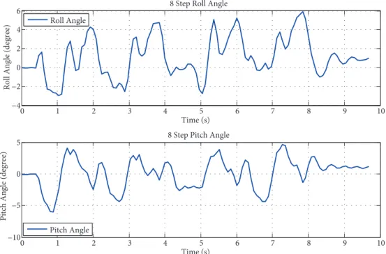
During the walking period, the biped robot’s trunk roll and pitch angles were measured by inertial measurement unit. Figure 7 shows the trunk angles change without any control except for motor PI control.
Although there are some irregularities in angle changes, the robot continues to walk steadily. Figure 8 shows the trunk angle changes with balanced foot contact controls.
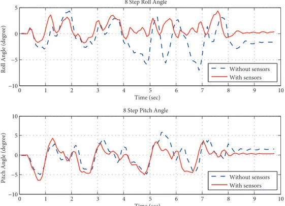
As shown in Figure 8, with that controller, angle change range from –6 to 6 degrees becomes the range from –4 to 4 degrees. More stable walking is achieved using balanced foot contact controls. Figure 9 shows the trunk angles change comparing with and without balanced foot contact controls.
0 1 2 3 4 5 6 7 8 9 10 −4 −2 0 2 4 6 Time (s)
Roll Angle (degree)
8 Step Roll Angle Roll Angle 0 1 2 3 4 5 6 7 8 9 10 −10 −5 0 5 Time (s) Pit ch Angl e (de gre e)
8 Step Pitch Angle
Pitch Angle
Figure 7. The trunk angles change without any control except for motor PI control.
0 2 4 6 8 10 12 −2 0 2 4 6 Time (s)
Roll Angle (degree)
8 Step Roll Angle
Roll Angle 0 2 4 6 8 10 12 −10 −5 0 5 Time (s) Pitch Angl e (de gre e)
8 Step Pitch Angle
Pitch Angle
Figure 8. The trunk angles change with balanced foot contact controls.
6. Conclusion and future works
In this paper, a walking pattern generation method based on LIPM and ZMP criterion for biped robots is presented. The walking pattern generation method suggested in the literature for big well-known humanoid robots is applied to a small biped robot RUBI, equipped with simple sensor structures and having relatively low complexity.
0 1 2 3 4 5 6 7 8 9 10 −10 −5 0 5 Time (sec)
Roll Angle (degree)
8 Step Roll Angle
Without sensors With sensors 0 1 2 3 4 5 6 7 8 9 10 −10 −5 0 5 10 Time (sec) Pitch Angl e (de gre e)
8 Step Pitch Angle
Without sensors With sensors
Figure 9. The trunk angles change comparison with or without balanced foot contact controls.
Robot trunk and feet movement equations were achieved as human-like walking by LIPM technique with Fourier series approximation and fixed reference ZMP trajectory. Experimental studies were evaluated by simple PI control structure.
The results of walking experiments showed that the robot trunk movements were in acceptable margins in both sagittal and coronal planes and the robot can walk stably. As a result, calculated trajectory equations with suggested assumptions were sufficient for the robot to walk without applying more complicated control algorithms that require more powerful processing units.
Unwanted swing foot moving effects and landing impact force influences seen in the experimental studies can be eliminated by some tunings of variables depending on the application in the control algorithm.
As future work, different ZMP references, swing foot dynamics considerations, and new LIPM – ZMP error compensation algorithm methods can be applied for more effective walking pattern generation. In addition, some control algorithms can be implemented to improve the control systems, such as landing impact compensation, early landing modification, and center of pressure (CoP) position controller.
References
[1] Hirai K, Hirose M, Haikawa Y, Takenaka T. Development of Honda humanoid robot. In: IEEE 1998 Robotics and Automation Conference; 16–20 May 1998; Leuven, Belgium. IEEE. pp. 1321-1326.
[2] L¨offler K, Gienger M, Pfeiffer F. Sensor and control design of a dynamically stable biped robot. In: IEEE 2003 Robotics and Automation Conference; 14–19 September 2003; Taipei, Taiwan. IEEE. pp. 484-490.
[3] Yamaguchi J, Soga E, Inoue S, Takanishi A. Development of a bipedal humanoid robot-control method of whole body cooperative dynamic biped walking. In: IEEE 1999 Robotics and Automation Conference; 10–15 May 1999; Detroit, MI, USA. IEEE. pp. 368-374.
[4] Kajita S, Kanehiro F, Kaneko K, Fujiwara K, Harada K, Yokoi K, Hirukawa H. Biped walking pattern generation by using preview control of zero-moment point. In: IEEE 2003 Robotics and Automation Conference; 14–19 September 2003; Taipei, Taiwan. IEEE. pp. 1620-1626.
[5] Kim JH, Oh JH. Realization of dynamic walking for the humanoid robot platform KHR-1. Advanced Robotics Journal 2004; 18: 749-768.
[6] Vukobratovic M, Borovac B, Surla D, Stokic D. Biped Locomotion: Dynamics, Stability and Application. Berlin, Germany: Springer-Verlag, 1990.
[7] Grizzle JW, Westervelt ER, Canudas WC. Event based PI control of an underactuated biped walker. In: 42nd IEEE 2003 Decision and Control Conference; 9–12 December 2003; Maui, HI, USA. IEEE. pp. 3091-3096.
[8] Chevallereau C, Bessonnet G, Abba G, Aoustin Y. Bipedal robots: Modeling, Design and Walking Synthesis. Wiltshire, Great Britain: Iste &Wiley, 2009.
[9] Kajita S, Kaehiro K, Kaneko K, Fujiwara K, Yokoi K, Hirukawa H. A real time pattern generator for bipedal walking. In: IEEE 2002 Robotics and Automation Conference; 11–15 May 2002; Washington, DC, USA. IEEE. pp. 31–37.
[10] Kajita S, Kanehiro F, Kaneko K, Yokoi K, Hirukawa H. The 3D linear inverted pendulum mode: A simple modeling for a biped walking pattern generation. In: IEEE/RSJ 2001 Intelligent Robots and Systems Conference; 29 October– 3 November 2001; Maui, HI, USA. IEEE. pp. 239-246.
[11] Kemalettin E, Okan K. Natural ZMP trajectories for biped robot reference generation. IEEE T Ind Electron 2009; 56: 835-845.
[12] Choi Y, You BJ, Oh SR. On the stability of indirect ZMP controller for biped robot systems. In: IEEE/RSJ 2004 Intelligent Robots and Systems Conference; 28 September–2 October 2004; Sendai, Japan. IEEE. pp. 1966-1971. [13] Vukobratovi¸c M, Borovac B. Zero moment point – thirty five years of its life. Int J Hum Robot 2004; 1: 157-173.
[14] Huang Q, Yokoi K, Kajita S, Kaneko K, Arai H, Koyachi N, Tanie K. Planning walking patterns for a biped robot. IEEE T Robotic Autom 2001; 17: 280-289.