An integrated process planning approach for CNC machine tools

I]dvanced

manufactudng

Technologg

An Integrated Process Planning Approach for CNC Machine Tools

M. Selim Akturk and Selcuk Avci

Department of Industrial Engineering, Bilkent University, Ankara, Turkey

In view of the high investment and tooling cost of a CNC machining centre, the cutting and idle times should be optimised by considering the tool consumption and the non-machining time cost components. In this paper, we propose a detailed mathematical model for the operation of a CNC machine tool which includes the system characterisation, the cutting conditions and tool life relationship, and related constraints. This new module will be a part of an overall computer-aided process planning system to improve the system effectiveness and to provide consistent process plans. A hierarchical approach is presented for finding tool-operation assignments, machining conditions, appropriate tool magazine organisation and an operations sequence which results in the minimum production cosL

Keywords: CNC; Machining parameters; Mathematical pro-

gramming; Optimisation; Process planning; Tool allocation

1. Introduction

A flexible manufacturing system (FMS) is a group of CNC machine tools interconnected by a material handling system and controlled by a computer system. FMSs are regarded as one of the most efficient methods to employ in reducing or eliminating problems in manufacturing industries. The key objectives of FMSs can be summarised as more rapid response both to market changes and to changing consumer demands in terms of product features, availability, quality and price; improved flexibility and adaptability; and low costs and high quality in design and production. In the FMSs literature, operational problems at the equipment level concerning operations sequencing, machining conditions optimisation and tool management are rarely addressed. There are several studies on system level problems that underly important aspects of operational problems. In most of these studies, the operational characteristics of the system components and the tool management concept have not been considered during the system modelling phase for simplifying the problem

Correspondence and offprint requests to: Dr M. S. Akturk, Department of Industrial Engineering, Bilkent University, 06533 Bilkent, Ankara.

formulation. Operational problems, such as the tool sharing, tool availability, loading duplicate tools, tool magazine capacity and tool life considerations should be taken into account for the reliable modelling of FMSs, or the absence of such crucial constraints may lead to infeasible results. Gray et al. [1] give an extensive survey on tool management issues for automated manufacturing systems, and also emphasise the fact that the lack of tooling considerations has often resulted in the poor performance of these systems. Furthermore, including these considerations at the equipment level, e.g. in process planning, provides an effective decision-making tool for short-term operational decisions for FMSs as discussed by Suri and Whitney [2].

Tooling considerations and the minimisation of the non- machining times are key factors for the effective utilisation of CNC machining eentres, and FMSs, as stated by Agapiou [3]. Kouvelis identified cutting tool utilisation as an important parameter for overall system performance [4]. In this study, the importance of tooling for FMSs is underlined. The cost of such tooling has been reported to be 25-30% of the fixed and variable costs of production. There also exist some studies [5-7] for the minimisation of the total non-machining time, at the system level, owing to changes in part mix. However, these studies assume constant processing times and tool lives, even though the actual tool wear, and the tool replacement frequency, is directly related to machining conditions selection. Gray et al. [1] reported that tools are changed ten times more often owing to tool wear than to part mix, because of the relatively short tool lives of many turning tools. In the

literature, we found no study that combines machining conditions optimisation, tool magazine arrangement and operations sequencing into a single study, or investigates the interactions between them. However, the importance of these concepts has been mentioned at both system and equipment level. We identified the need for such a problem formulation especially for computer-aided process planning and part programming. This study can be considered as a module in the framework of a fully integrated system [8,9].

2. Problem Definition

The aim of this research is to determine optimum machining conditions, operations sequences and tool magazine arrange-

ments to manufacture a batch of parts by a CNC machine on a minimum cost basis. The following assumptions are made to define the scope of this study:

There is a tool magazine attached to each CNC machine with a limited tool slot capacity.

For the machining operations, the cutting speed and the feedrate will be taken as the decision variables, and the depth of cut is assumed to be given as an input.

Each machining operation has a set of candidate tools from a variety of available tool types of limited quantities.

Machining condition optimisation for a single operation is a well-known problem and several methods have been developed for this in the literature. However, these methods consider only the contribution of machining time and tooling cost to the total cost of the operation, where the decision variables are the cutting speed and feedrate. In the multiple operations case, non-machining time components, such as tool switching between successive operations and tool inter- change, can have a significant impact on the total cost of production. Therefore, the total cost should be expressed in terms of both machining time and non-machining time components, and the tooling cost. Machining time, tin., is the

. . . . / J . .

t~me required to complete a turning operation. The relationship between the tool life, Tij, and machining time can be expressed as a function of the machining conditions by using an extended form of the Tailor's tool life equation. For the turning operation, the following expression has been derived for the machining time to tool life ratio, and a similar expression can be derived for other operations.

U# =--tmq = ~r Di Li d~d T~i 12 C. v(-~-% )¢-o-~)

All time-consuming events except the actual cutting oper- ation are called the non-machining time components. The following ones should be minimised since they are directly affected by the machining conditions selection and operations sequencing decisions:

Tool Switching Time is the time required to replace a worn tool with a new one, each tool might have a different switching time depending on whether or not the tool uses some special accessory.

Rapid Travel Motion Time is the time needed to relocate the tool from one point to another, e.g. from the tool magazine to the starting point of the cutting operation, which can be expressed as follows:

I

• v ~

Vs cts

where v~ and as are the speed and acceleration of the machine tool slides, respectively, and A,,y is the shortest linear distance between the points x and y.

Tool Interchanging Time is the time necessary to move a tool from the toot holder to the tool magazine and replace it, or vice versa.

Though there may be other distinct non-machining time components, such as tool tuning, spindle acceleration/deceler- ation, workpiece loading/unloading, we consider only the ones that can be expressed either as a function of the machining condition or the operations sequence, or those that can vary between the different tool and operation pairs.

A general mathematical formulation is given below. In this formulation, the objective function is expressed as a function of machining conditions selection, operations sequencing and tool assignment, where M gives the set of alternatives, and is the set of allocated tools, which is a subset of the available tool set, J. There are three types of constraints, namely, system, tool related and machining operation constraints. The first two sets of constraints represent the system constraints which are the tool magazine capacity limitation and the operation-tool assignments. The tool availability and tool life constraints are the tool related constraints which ensure that the solution will not exceed the available quantity on hand and the available tool life capacity for any tool type. The last two constraints are the machining operation constraints. The surface roughness represents the quality requirement for the operation and the machine power constraint limits the machine tool to operations which do not cause damage.

min

m E M = ( m l f ( v , f , w J C . J ) } Ctm(m) Subject to:

~, aj <-- TM (tool magazine

j ~ constraint)

xij = 1 V i E I (tool assignment

j ~ constraint)

~, xij n,~j <- t~ V j ~ J (tool availability

iex constraint)

xij Uij -< 1 V j E J (tool life

iel constraint)

Ca v,~-~, d~ -< S Fm~ V i ~ I, j E J (surface roughness constraint) Cm vb ~ d~ <- H Pm~ V i E I, j E J (machine power

constraint)

This is a nonlinear mixed integer programming (MIP) formulation having several interrelated decisions to be made at different levels.

3. Proposed Hierarchical Approach

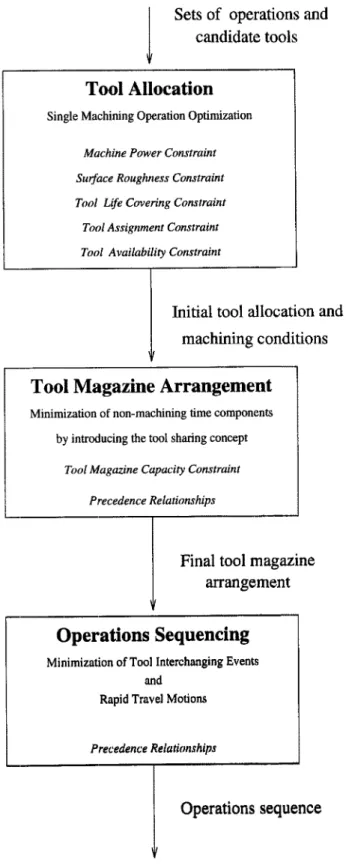
The constraints and the decision variables for machining conditions, tool and operation assignments, and operations sequence interact with each other. At the first level of the proposed hierarchical approach, as shown in Fig. 1, the tool allocation problem will be solved in conjunction with single machine optimisation. After finding the operation-tool assign- ments, which reduces the candidate tool set for each operation

Sets of operations and

candidate tools

Tool Allocation

Single Machining Operation Optimization

Machine Power Constraint Surface Roughness Constraint Tool Life Covering Constraint Tool Assignment Constraint Tool Availability Constraint

Initial tool allocation and

machining conditions

Tool Magazine Arrangement

Minimization of non-machining time components by introducing the tool sharing concept

Tool Magazine Capacity Constraint Precedence Relationships

Final tool magazine

arrangement

Operations Sequencing

Minimization of Tool Interchanging Events

and

Rapid Travel Motions

Precedence Relathmships

Operations sequence

Fig. 1. Flowchart of the proposed hierarchy.

to a single tool, the solution will be improved by considering other decision variables and the feasibility constraints. As indicated in the flowchart, the precedence and tool magazine capacity constraints are relaxed at the first level, then the feasibility of the solution is checked at the second level while a further improvement of the current solution is sought by

an algorithm which allows tool sharing among the operations to minimise non-machining time. In the third level, the operations sequencing decision will be made by considering the tool-operation assignments and tool sharing events to minimise rapid travel motion and tool interchanging times.

3.1 Single Machining Operation Optimisation

(SMOP)

In SMOP, the objective function includes the tooling cost and operating cost due to the machining time, and it is possible to impose the machining operation constraints on that problem together with a tool life constraint as defined below: Minimise

Cm~;

= C, v~l fi] -1 + C 2 p!ftj-1) f

vq,~j > 0

(tool life constraint) (machine power constraint) (surface roughness constraint)

Di Li d~d Ctj

c2 =

12c~

• r Di Li dTJpij Cm d~ C~

G - 12Cj ' C ' - H P m ~ x " C ' ~ - S F m ~ ,

The above problem can be solved by using geometric programming (GP) in a reasonable computational time [10,11]. The associated GP-Dual problem for the above formulation is given below. The objective function for the dual problem is still a nonlinear one, but the constraints of the dual formulation are well-defined linear equations.

Maximise

_Q*

_{| c I | Y I ~ v I (C~)Y3(C~)Y4(c:)Y5}

Subject to:

Y 1 + r 2 = l

- h + ( o~j - 1 ) r2 ÷ ( ,~j - 1 ) g3 + b r4 + g Ys = O - Y~ + ( f 3 j - 1 ) Y2 + (f3]- l ) Y3 + c Y4 + h Y s = O

Y,, Y2, Y3, Y4, Ys >- o

The dual problem is solved by using the complementary slackness conditions in conjunction with the primal and dual constraints. Each of the constraints of the primal problem can be either loose or tight at the optimality. Therefore, the principle used to solve this dual problem is to check every possible constraint in the primal problem and then to solve the corresponding dual. If a dual feasible solution is found then the corresponding primal solution can be evaluated in terms of its decision variables, and consequently the primal feasibility of the solution can be checked. At the optimality,

the corresponding solution should be feasible in both the dual and primal problems, and the objective function value for both problems should be the same. Since we have three constraints in the primal problem, there are eight different cases for the dual problem, but only six of them are feasible as stated below.

Theorem 1. In the constrained SMOP, at least one of the surface roughness or machining power constraints must be tight at the optimal solution.

The exact solution for the extended version of SMOP can be found by solving each of the aforementioned six cases for the worst case. In each case, solving a linear system of at most three equations and unknowns yields the solution very quickly, regardless of any computational complexity issues, using the proposed hierarchical scheme.

3.2 Tool Allocation

The following heuristic is proposed to reduce the initial candidate tool set to a single tool for every operation, by considering the tool availability constraint, and to determine the cutting conditions for every tool and operation pair. After finding the best tool allocation, tool sharing will be introduced to improve the current solution at the second level.

Step 1. For every possible operation, solve SMOP using the procedure defined in Section 3.1. Calculate the number of parts that can be manufactured, P0 = [1/U0J, and the number of tools required, ntis = [NB/Pij].

Step 2. In the multiple operation case, a lower total cost value can be obtained while increasing the cost of SMOP owing to a possible decrease in operating costs. The following cost measure is developed to evaluate alternative tools for an operation, where the first term represents the cost of SMOP, and the second and third terms account for operating costs due to the non-machining time components and the waste of tool life cost, respectively.

-Cij = NaC~,s+ C o [ ( n t q - ~)ts]k- tt,]

+ C, s [NdpoJ (1 - P o U,j)

Let ]p be the set of primal tools that give the minimum cost measure for every operation and I s be the set of operations for every primal tool.

Step 3. For operations having only one candidate tool, allocate tool j to operation i. Update sets I and J, and reduce the available number of tools, t], for further allocations.

Step 4. For every J E Je, calculate the total tool requirement, R~ = E ~ r nt o. If Rj - t h allocate tool j for Vi E/~, and update ~,, J, and ti. Otherwise, calculate the deficit tool amount, ~i = Rj - tj, and the perturbation ratio, pj -- ~j/Ri. Step 5. Starting from the most critical tool, i.e. the highest Pi value, span the possible reductions in the tool requirement, 7r E II~j = F o U Aii, for every operation of j, to satisfy the tool availability constraint. For every perturbation Ir E Fq, solve SMOP again to find the new machining conditions, number of tools, nt~.., and the resulting cost, ~-~q. The alternative

q , .

tools, denoted by A~ i, are also considered because an increase

in the cost of SMOP owing to a reduction of tool usage might justify the use of one of them. For every ~r ~ II0, calculate the corresponding cost increment, as follows:

For every perturbation Ir E FO, the cost increment is A~-~ = -- U//j, where ~ corresponds to the initial cost measure found at Step 2.

For every alternative tool ~r E A~, the cost increment is ~ T = C/~, - ~ + Ixj, ntr,, where C/~¢ corresponds to the cost for alternative tool j ' an~ pq, is the opportunity cost of using an_ alternative_ deficit tool, which is equal to IX1, = maxk%, (C~j, - ~ j , } for the deficit tools, or zero otherwise. Step 6. Solve the following 0-1 IP to find the best perturbation combination that satisfies the related tool availability con- straints with a minimum total cost increment.

Minimise E ~] z7 A ~ Subject to: i% ~en o

z T = l V i E I j " r r E I l q E E zrn~,<--tJ i% "~hs Z ~ z~"=<-ts' t ~tlj, V j ' E ( O J i ] / j i~l] Ir~Aij \ Clj / i

where z ] is a 0-1 binary variable which is equal to 1 if the wth perturbation is selected for operation i ~ Ij. In the above model, the first constraint ensures that a single perturbation will be selected for each operation, and the second constraint ensures that the tool usage will be limited by the available quantity. The third constraint identifies the set of alternative tools for each operation and guarantees that the tool availability constraint for these alternative tools will also be satisfied. Step Z If an alternative tool, which has not been previously used, is allocated for some operation, the additional cost of Ca = Co Nn t~; will be included in the cost measure to compensate for the tool changing owing to the introduction of this new tool type, and Step 6 is revisited. Otherwise update sets I, J and Jp, and reduce the available number of tools for every allocated tool type. If the set Jp 4= 0 go to Step 5, otherwise stop.

This algorithm uses the extended version of SMOP initially, then a new cost measure is proposed to handle the case of multiple operations by considering the related non-machining time components and tool waste cost. Finally, the best operation-tool pairs are found that satisfy both the tool availability and tool life limitations.

3,3 Tool Magazine Arrangement

After the tool allocation procedure, the tool magazine capacity constraint and tool sharing should be considered to avoid any infeasibility due to the initial tool loading. Moreover, non- machining times can be further minimised by introducing tool sharing. At the beginning, a violation of the tool magazine capacity constraint can be identified by assuming total tool

sharing for every tool type in the final tool allocation. The tool life constraint may also create a need for loading duplicate tools in the tool magazine. The following heuristic algorithm is proposed to find the best tool magazine arrangement. Step 1. For tool types having only a single operation assign- ment, a single slot should be allocated in the magazine, such that aj = 1, and j El.

Step, 2. For tools having more than one operation in their assignment set, determine the possible tool requirement levels, I ELy. Create a set of operations that can be performed and generate a duplicate tool for this requirement level.

Step, 3. For tools in set J \ ], determine the feasible operation- tool allocation resulting in the minimum tool slot requirements, ¢i, and check the following tool magazine capacity constraint:

cj <- T M - ~ aj jE:r~J j d

If the above constraint is violated, then the problem is infeasible. Otherwise find the possible tool slot requirements, aj. Determine the feasible operation-tool assignment giving the best tool sharing as the alternative allocation, p E Pj, for each tool slot number aj.

Step 4. Evaluate the following cost measure, ~ , for every alternative tool type j, where Ark, Czk are the set of adjacent operations and the set of all operations of the kth duplicate tool of requirement level l, respectively:

l ~ L j k E K 1 (i,i Alk

+ ~ (tr1~+t,,+2tcj)J+Co[(t,-s,)-a,]ts j iE(ClkkAlk)

+ [Coajt,] + Ctj(tj-sj)

In the above cost measure, the machining cost is excluded since it has been fixed by the tool allocation algorithm. In the first term, the rapid travel motion (RTM) times and the tool interchanging times are found by considering the tool sharing information which is embedded in set A~k. The second term also accounts for the RTM and tool interchanging times of the distinct operations excluded by set A~k. The other terms represent the tool switching, loading and tooling costs, respectively. Briefly, this cost expression includes all the non- machining time components and the tooling costs since they are closely related to the tool magazine arrangement and the tool sharing.

Step 5. Determine the best tool arrangement for every tool type in J \ J by solving the following 0-1 IP, where b~ is a 0-1 binary variable, which is equal to 1 if the pth alternative arrangement of tool j is selected:

Minimise ~ ~ b,e Cl ,j jES~f p E P j Subject to: ~ ~ = 1 V j E j \ J ' p~t'j

E E b~a~<--TM-Ea,

In this formulation, the first constraint requires that only one of the alternatives will be selected and the second constraint ensures that total tool slot requirements of the entire tool magazine arrangement will not exceed the tool magazine capacity.

In this level, the tool magazine arrangement algorithm is developed to impose the tool magazine capacity on the problem and to search for the tool sharing and tool duplication possibilities for further improvement to the operation-tool allocation. Furthermore, operations sharing the same tool are aggregated into a single virtual operation and a partial operations sequence is generated at this level.

3.4 Operations Sequencing

After fixing the operation-tool allocations and the tool magazine arrangement, the operation sequencing decision remains to be made. Tool interchanging and rapid travel motion times are the only variables to be minimised at this level. This sequencing decision is transformed into a network model, in which nodes correspond to the several phases of a workpiece which is initially of raw material in state o, and then every cutting operation changes the state of the workpiece. At the end, the final state having m operations is denoted by the node m + 1. Cutting operations are presented by the arcs and every arc will have a cost value corresponding to the sum of non-machining times due to state transitions. Furthermore, at each state, a set of operations, Si, that can be done at state i, is defined by imposing the precedence relations between the operations. Our objective is to find the minimum path from root node o to final node m + 1. The following algorithm is proposed to make a full enumeration by examining all feasible alternatives.

Step 1. For tools having a sequence of adjacent operations, define a new operation by taking the starting point of the first operation of this chain as the starting point, and the endpoint of the last operation as the endpoint of the aggregated volume.

Step 2. Calculate the cost of arcs from root node o to state 1 as follows:

Co, i = tc] ~- trf, i , where i E S~ and xq = 1

Step 3. For every intermediate state n, where n E (1 . . . m - 1}, calculate cost of the arc directed from state S, to S,÷1, where i' E S,, i E S,+1, andj' and] are their correspond- ing tools, respectively:

tt, j+t~j,+tg +trr, i i f j ' ~ j Ci, i : [tr i-'

t'.~ ifj' = j

Step 4. Calculate the cost of arc from state m to state m + 1 as follows:

v,

v:

v,

v, t

v,

/ " \ v .

v,~

T

v~,,

--4 in. @ =3.5 in. qb =2.5 in. qb =1.5 in. • =2 in.

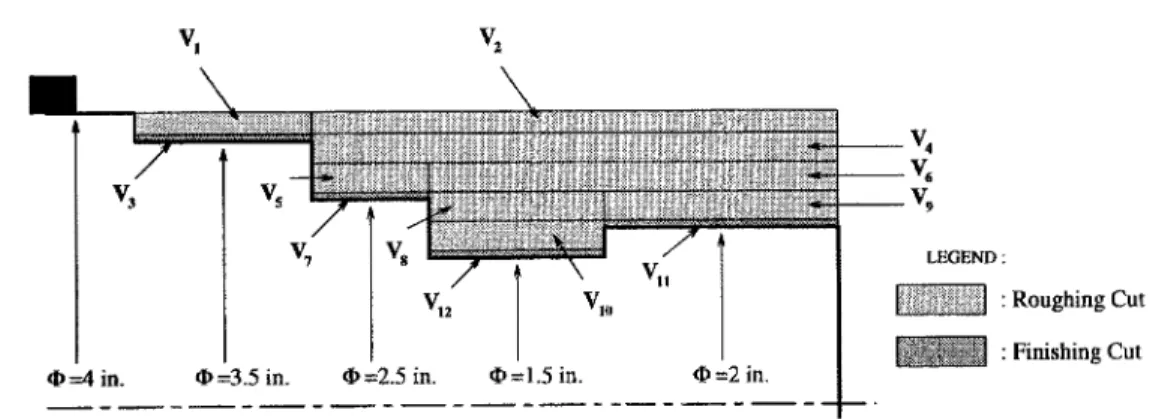
Fig. 2. Machinable volume presentation.

_ _ v ,

L E G E N D :

: Roughing Cut : Finishing Cut

Table 1. Machinable volume data.

V D~ L~ d~ SFm~, V D, Li d~ S F ~ V1 4 3 0.2 300 V7 2.6 2 0.05 50 V2 4 9 0.2 400 V8 2.6 3 0.25 400 V3 3.6 3 0.05 75 V9 2.6 4 0.25 300 V4 3.6 9 0.25 400 Vlo 2.1 3 0.25 300 115 3.1 2 0.25 300 Vtl 2.1 4 0.05 40 Va 3.1 7 0.25 400 V12 1.6 3 0.05 30

Ci,m+l "~ try+ tcj, where i E S m

Step 5. Calculate total cost for every path from root node o to leaf node m + 1 and pick the minimum cost path as the operations sequence.

4. A Numerical Example

In this section, an example part (illustrated in Fig. 2) is studied. It has twelve prespecified machinable volumes with the geometrical data and the required surface qualities given in Table 1. There are six different tool types available whose technological parameters and the other input data are presented in Tables 2 and 3, respectively.

The candidate tools for each operation are specified by the ~ l l o ~ n g O - I m a t r i x Y : 0 0 1 0 0 0 1 0 - 0 0 1 0 0 0 1 0 1 1 1 1 1 1 1 1 Y = 1 1 0 1 1 1 0 1 " 1 1 1 1 1 1 1 1 0 0 0 0 0 0 1 0 I n t ~ f i r s t t w o ~ e p s o f t h e 0 0 1 1 0 0 1 1 r 1 1 0 1 1 0 0 0 0 1 1

tool allocation algorithm, the

Table 3. Tooling information.

/"1 T2 T3 T4 T5 T~ 0.75 0.75 0.75 0.75 1 0.75

~ 1 1 1 1 1.5 0.75

tj 2 3 20 10 4 2

Ctj 0.50 0.70 0.70 0.70 0.75 0.75

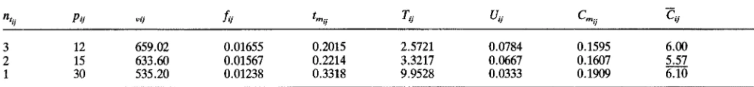
best machining conditions for every possible o p e r a t i o n - t o o l pair is determined for different nt,j values. In Table 4, this procedure is illustrated for the v o l u m e - l l and tool-6 pair, i.e. operation (11,6). Here, one should note that we found a better solution by decreasing the tool usage since the increase in the cost of SMOP has been justified by the decrease in the overall cost. This clearly shows the importance of the proposed cost measure, Cij, compared to the SMOP approaches, which does not consider the non-machining time components and the tool waste cost.

In step 2, the following sets are formed by using the best machining operation conditions for every possible pair: 13 = {1,2,4,5,6,8,9,10), 15 = {3}, 16 = {7,11,12} and Jp = (3,5,6}. Since there is no operation having a single candidate tool, we skip step 3 of the algorithm. In step 4, we determine the tools for the set Je for which the tool availability constraint is violated, as follows:

Table 2. Technological exponents and coefficients of the available tools.

T a 13 ~/ Cj b c e Cm g h y (7, T1 4;0 1.40 1.t6 40960000 0.91 0.78 0.75 2.394 -1.52 1.004 0.25 204620000 T2 4.3 1.60 1 . 2 0 37015056 0.96 0.70 0.71 1.637 -1.60 1.005 0.30 259500000 T3 3.7 1.28 1 . 0 5 11001020 0.80 0.75 0.70 2.415 - 1.63 1.052 0.30 205 740000 T4 4.1 1.26 1 . 0 5 48724925 0.80 0.77 0.69 2.545 -1.69 1.005 0.40 204500000 Ts 3.7 1.30 1 . 0 5 13767340 0.83 0.75 0.73 2.321 -1.63 1.015 0.30 203500000 7"6 4.2 1.65 1.20 56158 018 0.90 0.78 0.65 1.706 - 1.54 1.104 0.32 211825 000

Table 4. Finding the minimum cost for operation (11,6).

nti] Pi 1 vii fij tmij T~i Ui/ Cmij Cij

3 12 659.02 0.01655 0.2015 2.5721 0.0784 0.1595 6,00 2 15 633.60 0.01567 0.2214 3.3217 0.0667 0.1607 5.57 1 30 535.20 0.01238 0.3318 9.9528 0.0333 0.1909 6.10 NB = 30 parts, Co = $0.5/min, and HPm~x = 5 h.p.

R3 := nq. 3 + nt2. 3 + n~4, 3 + nts. 3 + ntr. a + nts. 3 + ntg, 3 -~ nqo.3 = 3 + 6 + 6 + 2 + 4 + 2 + 3 + 2 = 2 8 > t 3 = 2 0

R5 = nt3, 5 = 2 < t5 = 4

R6 =ntT, 6 + nql.6 + nt12,6 = i + 2 + 1 = 4 > t6 = 2

For the tool-5, there exists an excess of 2 tools, so this tool and its corresponding volume are appended in the following reservation sets and the available quantity on hand is updated: 7 = {3}, 2 = {5} and t5 = 2. For the other tools, the deficit ratios are as follows:

28 - 20 4 - 2 P 3 - 28 ---0,2857, 9 6 = ~ = 0 . 5

From the above values, tool-6 is found as the most scarce resource, therefore in the next step first the allocation of this tool is completed, then we will continue with tool-3. For this propose, all possible perturbations of tool-6 for its operation assignments are generated as explained in step 5. A n example perturbation set is given for operation (11,6) of tool-6 in Table 5, where the cases rr = 2 and ~ = 3 correspond to the use of secondary tools, tool-1 and tool-2, respectively, instead of the primary tool of tool-6. For the allocation of tool-6, a 0-1 IP is solved to find the best combination of the possible perturbations for the operations 7, 11 and 12 as discussed in 0 = 1. Therefore step 6. The optimal solution is z~ = z ~ = z ~

tool-5 is used for the manufacturing of volume-7 instead of tool-6, and a reduction of a single tool-6 in the processing of the volume-ll, leaving the original solution for the volume- 12 without any reduction in the usage of tool-6. For the secondary deficit tool, tool-3, the same IP model has been solved with the new parameters and the possible perturbations which were generated after the allocation of tool-6 and updating the related sets and tool availabilities. The resulting Table 5. Alternative allocations of volume 11.

final tool allocations with the corresponding machining con- ditions are given in Table 6.

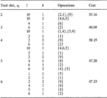
In the first step of the tool magazine arrangement algorithm, a single tool slot is reserved for tool-4 which has been allocated for volume-4. In step 2, pre-processing is applied to the input data to detect the infeasible cases and to reduce the problem size for the following steps. In step 3, we determine the minimum tool slot requirement, ei, for each tool type to justify the initial feasibility of the problem. For this particular example, we found that E 3 = 2 , ~5 = 2 and ~6 = 1. The tool magazine capacity constraint is checked and the minimum slot allocations are proved to be feasible. In the same step, a further processing is made to indicate the precedence relationships which give the best operation-tool assignment for a given number of tool slots. The precedence relations for the operations of tool-3 are illustrated in Fig. 3. After determining the possible allocations of all tools, a cost figure for each alternative is calculated in step 4. The possible alternative arrangements of tool 3 are given in Table 7 with the corresponding tool sharing combinations, tool duplication requirements and their respective costs. Finally, the best arrangement is selected in step 5 as summarised in Table 8, where the tool sharing events are presented by the ordered sets in the operations column. For example, tool 3 has two duplicates at requirement level 10 and the second duplicate is shared by the operations 4, 6 and 5 in the given operations sequence. This partial sequence, denoted by the aggregate operation 4 + , is found by considering the minimum travelling distance and also preserves the precedence relationships.

The third level of the proposed method is the operation sequencing which minimises the total rapid travel motion and tool interchanging times. Since the previous level has resulted in tool sharing for some of the adjacent operations, these operations can be considered as the aggregate volumes to be

0 6 15 6 3 3 . 6 0 0 . 0 1 5 6 7 0.2214 3.3217 0.0667 0.1607 2 5.57 0 1 6 30 5 3 5 . 2 0 0 . 0 1 2 3 8 0.3318 9.9528 0.0333 0.1909 1 6.10 0.53

'lr T Pij vi i' fly, tmij, Tij, Vii, C, nij , n~., ~iy, A'C~

2 1 15 651.89 0 . 0 0 7 9 9 0.4222 6.3335 0.0667 0.2445 2 8.21 2.64 3 2 10 538.40 0 . 0 0 9 0 8 0.4495 4.4947 0.1000 0.2947 3 10.09 4.52

Table 6. Final tool allocation and the machining conditions.

V T nt o vii fo tin# T# Uij Cm# -Co

1 3 2 266.13 0.02565 0.4599 6.8990 0.0667 0.2766 9.17 2 3 6 256.73 0.03189 t . 1 ~ 5.9650 0.1929 0.7103 23.83 3 5 2 528.39 0.02624 0.2038 3.0575 0.0667 0.1519 5.8t 4 3 5 236.50 0.02635 1.3604 8.1623 0.1667 0.7969 25.91 5 3 1 245.79 0.02128 0.3102 9.3053 0.0333 0.1784 5.85 6 3 4 242.92 0.02747 0.8510 7.0095 0.1214 0.5105 17.00 7 5 1 555.22 0.01905 0.1286 3.8584 0.0333 0.0893 3.43 8 4 2 214.75 0.03025 0.3142 4.7125 0.0667 0.2038 6.99 9 3 2 259.98 0.02321 0.4509 6.7640 0.0667 0.2721 9.04 10 5 2 270.56 0.02181 0.2793 8.5375 0.0327 0.1642 5.69 11 6 2 535.20 0.01238 0.3318 9.9528 0.0333 0.1909 6.10 12 6 2 639.16 0.01222 0.1608 4.8244 0.0333 0.1054 3.54

@

®

Fig. 3. Precedence relationship among the operations of tool-3.

Table 7. Alternative arrangements of tool-3.

Tool slot, a i 1 k Operations Cost 2 10 1 {2,1},{9} 35.16 10 2 {4,6,5} 4 1 {6} 3 6 1 {2} 40.09 10 1 {1,4},{5,9} 2 1 {1} 4 2 2 {9} 38.19 6 1 (2} 10 1 {4,6,5} 2 1

{1}

v, = 5 in./s, % = 5 in./s 2, t~j = 3 s, TM = i0 and f = (0,0,20) in inches

manufactured with the s a m e tool. T h e possible nodes and the cost of each arc a r e given in T a b l e 9 and the following operations s e q u e n c e is f o u n d to be t h e best o n e (2 + - + 4 + - + 9 - + 8 --+ 7 --+ 10 --+ 3 --+ 11+). T h e r e f o r e the final operations s e q u e n c e is as follows:

2--+ 1--+4--+ 6 - - + 5 - - + 9 - - + 8 - - + 7 - - + 1 0 - + 3--+ 11--+ 12 In s u m m a r y , t h e initial solution of S M O P was worse than the p r o p o s e d cost m e a s u r e for the multiple o p e r a t i o n case as

Table 8. Final operation-tool assignments and tool magazine arrange-

ment.

Tool type Duplicate t k Operations Cost

3 1st duplicate 10 1 {2,1},{9} 35.16 2nd duplicate 10 2 {4,6,5} 4 Single 2 1 {8} 6.42 5 1st duplicate 1 1 {7) 14.29 2nd duplicate 3 1 {3},{10} 6 Single 2 1 {11,12} 6.60

Table 9. Total times between the operations.

f v+~ v3 v+4 v7 v8 v9 vlo v ~ f oo 8.79 8.10 8.78 8.18 8.39 8.78 8.39 8.78 V~ 8.02 ~ 16.12 16.80 16.20 16.41 16.80 16.41 16.80 113 8.02 16.81 oo 16.80 16.20 16.41 16.80 16.41 16.80 V~ 8.09 16.88 16.19 oo 16.27 16.48 16.87 16.48 16.87 V7 8.09 16.88 16.19 16.87 o~ 16.48 16.87 16.48 16.87 1/8 8.18 16.97 16.28 16.96 16.36 ao 16.96 16.57 16.96 1/9 8.39 17.18 16.49 17.17 16.57 16.78 0o 16.78 17.17 111o 8.18 16.97 16.28 16.96 16.36 16.57 16.96 oo 16.96 V~il 8.18 16.97 16.28 16.96 16.36 16.57 16.96 16.57

indicated in T a b l e 4, and it was also infeasible due to the tool availability constraint resulting f r o m t h e c o n t e n t i o n a m o n g the operations for a limited n u m b e r of tools.

5. Conclusion

A hierarchical approach is p r e s e n t e d for solving machining conditions optimisation, tool magazine a r r a n g e m e n t and operations sequencing p r o b l e m s for a C N C machine. Briefly, at t h e first level, t h e tool allocation p r o b l e m is solved by relaxing t h e tool magazine capacity constraint. T h e tool and o p e r a t i o n assignments are fixed and the machining conditions are d e t e r m i n e d by assuming no tool sharing occurs a m o n g the operations. T h e results of S M O P h a v e b e e n e x t e n d e d to h a n d l e the case of multiple o p e r a t i o n s by considering t h e related n o n - m a c h i n i n g t i m e c o m p o n e n t s and tool duplication. In the second level, the tool magazine capacity constraint and

precedence conditions are imposed on the problem and tool sharing is considered for possible improvements. The final composition of the tool magazine is fixed by considering the arrangement of each tool type, and an operations sequence is found for the operations which share the same tool. Finally, the operations sequencing decision is made at the third level to minimise the rapid travel motions and tool interchange tin~tes which use the information on final tool magazine arrangement and the operation assignments.

The proposed hierarchy integrates the tool allocation and tool magazine arrangement problems with the machining conditions optimisation problem to minimise the total pro- duction cost where alternative tools can be used for each operation. As a result, we not only improve the overall solution by exploiting the interactions between different decision-making problems, but also prevent any infeasibility that might occur at the system level owing to contention among the operations for a limited number of tool types by considering tool availability, tool life, precedence and tool magazine capacity limitations. As indicated in the example problem, a decision made at a higher-level without considering its impact on the lower-levels can lead either to infeasible or inferior results when we consider both the constraints and parameters of the tower-level problems. This model is considered as part of a fully automated process planning system. Therefore interfacing this model with the other modules is an important problem to be studied since effective phmning models must take into account system limitations, tool changing times, tool sharing, loading duplicate tools, and tool lives.

2. R. Suri and C. K. Whitney, "Decision support requirements in flexible manufacturing", Journal of Manufacturing Systems 3(1), pp. 61-69, 1984.

3. J. S. Agapiou, "Sequence of operations optimization in single- stage multi-functional systems", Journal of Manufacturing Systems, 10(3), pp. 194-208, 1991.

4. P. Kouvelis, "An optimal tool selection procedure for the initial design phase of a flexible manufacturing system", European Journal of Operational Research, 55(2), pp. 201-210, 1991.

5. J. F. Bard, "A heuristic for minimizing the number of tool switches on a flexible machine", lEE Transactions, 20(4), pp. 382-391, 1988.

6. Y. Crama, A. W. J. Kolen, A. G. Oerlemans and F. C. R. Spieksma, "Minimizing the number of tool switches on a flexible machine", The International Journal of Flexible Manufacturing Systems, 6(1), pp. 33-54, 1994.

7. C. S. Tang and E. V. Denardo, "Models arising from a flexible manufacturing machine, Part I: Minimization of the number of tool switches", Operations Research, 36(5), pp. 767-777, 1988. 8. S. H. Yeo, Y. S. Wong and M. Rahman, "Knowledge based

systems in the machining domain", International Journal of Advanced Manufacturing Technology, 6(1), pp. 35-44, 1991. 9. M. Kalta and B. J. Davies, "Product representation for an expert

process planning system for rotational components", International Journal of Advanced Manufacturing Technology, 9(3), pp. 180-187, 1994.

10. M. S. Bazaraa, H. D. Sherali and C. M. Shetty, Nonlinear Programming Theory and Algorithms, 2nd edn. John Wiley and Sons, 1993.

11. B. Gopalakrishnan and F. AI-Khayyal, "Machine parameter selection for turning with constraints: An analytical approach based on geometric programming", International Journal of Production Research, 29(9), pp. 1897-1908, 1991.

References

1. A. E. Gray, A. Seidmann and K. E. Stecke, "A synthesis of decision models for tool management in automated manufacturing" , Management Science, 39(5), pp. 549-567, 1993.

Nomenclature

speed, feed, depth of cut exponents for tool j the number of tool slots allocated for tool type j Taylor's tool life constant for tool j

specific coefficient and exponents of the machine power constraint

operating cost of the machine tool ($/min)

specific coefficient and exponents of the surface roughness constraint

cost of the tool j (S/per tool)

diameter of the generated surface (in.) depth of cut for operation i (in.) feedrate for operation i using tool j

maximum allowable machine power for all operations set of all operations

set of assigned operations set of the available tools set of the allocated tools set of the arranged tools

length of the generated surface (in.) batch size SFmax T M

to,

t,,

%

maximum allowable surface roughness for the volume i

the capacity of the tool magazine tool changing time for tool j (min)

tool magazine loading time for a single tool j (rain) rapid motion time for moving the tool from a fixed point to the starting point of the operation i (rain) rapid motion time for moving the tool from the endpoint of the operation i to the fixed changing point

(min)

tool switching time for the tool j (min) cutting speed for the operation i (f.p.m.) operations sequence vector

0-1 binary variable which is equal to 1 if tool j is used in operation i