1554 IEEE TRANSACTIONS ON COMPUTERS, VOL. 37, NO. 12. DECEMBER 19x8
Iterative Algorithms for Solution of Large Sparse
Systems of Linear Equations on Hypercubes
CEVDET AYKANAT, FUSUN OZGUNER, MEMBER, IEEE, FIKRET ERCAL, STUDENT MEMBER, IEEE, A N D
PONNUSWAMY SADAYAPPAN, MEMBER, IEEE
Abstract-Solution of many scientific and engineering prob- lems requires large amounts of computing power. The finite element method [l] is a powerful numerical technique for solving boundary value problems involving partial differential equations in engineering fields such as heat flow analysis, metal forming, and others. As a result of finite element discretization, linear equations in the form A x = b are obtained where A is large, sparse, and banded with proper ordering of the variables x. In
this paper, solution of such equations on distributed-memory message-passing multiprocessors implementing the hypercube [2]
topology is addressed. Iterative algorithms based on the Conju-
gate Gradient method are developed for hypercubes designed for coarse grain parallelism. Communication requirements of differ- ent schemes for mapping finite element meshes onto the proces- sors of a hypercube are analyzed with respect to the effect of communication parameters of the architecture. Experimental results on a 16-node Intel 386-based iPSC/2 hypercube are presented and discussed in Section V .
Index Terms-Finite element method, granularity, hypercube, linear equations, parallel algorithms
I. INTRODUCTION
OLUTION of many scientific and engineering problems
S
requires large amounts of computing power. Withadvances in VLSI and parallel processing technology, it is now
feasible to achieve high performance and even reach interac-
tive or real-time speeds in solving complex problems. The
drastic reduction in hardware costs has made parallel com- puters available to many users at affordable prices. However,
in order to use these general purpose computers in a specific
application, algorithms need to be developed and existing algorithms restructured for the architecture. The finite element
method [ I ] is a powerful numerical technique for solving
boundary value problems involving partial differential equa- tions in engineering fields such as heat flow analysis, metal forming, and others. As a result of finite element discretiza- tion, linear equations in the form A x = I, are obtained where
A is large, sparse, and banded with proper ordering of the
Manuscript received February 12, 1988; revised July 11, 1988. This work was supported by an Air Force DOD-SBIR Program Phase I1 (F33615-85-C- 5198) through Universal Energy Systems, Inc., and by the National Science Foundation under Grant CCR-870507 1.
C. Aykanat and F. Ercal were with The Ohio State University, Columbus, OH 43210. They are now with the Department of Computer and Information Science, Bilkent University, Ankara, Turkey.
F. Ozguner is with the Department of Electrical Engineering, The Ohio State University, Columbus, OH 43210.
P. Sadayappan is with the Department of Computer and Information Science. The Ohio State University, Columbus, OH 43210.
IEEE Log Number 8824085.
variables x . Computational power demands of the solution of
these equations cannot be met satisfactorily by conventional sequential computers and thus parallelism must be exploited. The problem has been recognized and addressed by other
researchers [ 1]-[4]. Attempts to improve performance include
a special-purpose finite element machine built by NASA [SI. Distributed memory multiprocessors implementing mesh or hypercube topologies are suitable for these problems, as a regular domain can be mapped to these topologies requiring
only nearest neighbor communication [ 11. However, a closer
look at message-passing multiprocessors reveals that speedup cannot be achieved that easily because of the communication overhead.
Methods for solving such equations on sequential computers
[6] can be grouped as direct methods and iterative methods.
Since the coefficient matrix A is very large in these applica-
tions, parallelization by distributing both data and computa- tions has been of interest. The Conjugate Gradient (CG) algorithm is an iterative method for solving sparse matrix equations and is being widely used because of its convergence properties. The sparsity of the matrix is preserved throughout
the iterations and the CG algorithm is easily parallelized on
distributed memory multiprocessors [ 1
I.
In this paper, solution of such equations on distributed-
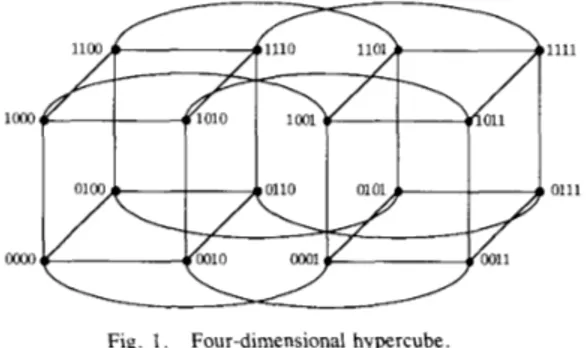
memory message-passing multiprocessors implementing the hypercube [2] topology is addressed. In such an architecture, communication and coordination between processors is achieved through exchange of messages. A d-dimensional
hypercube consists of P = 2 d processors (nodes) with each
processor being directly connected to d other processors. A
four-dimensional hypercube with binary encoding of the nodes
is shown in Fig. 1. Note that the binary encoding of a
processor differs from that of its neighbors in one bit. The processors that are not directly connected can communicate through other processors by software or hardware routing. The maximum distance between any two processors in a d- dimensional hypercube is d . It has been shown that many other topologies such as meshes, trees, and rings can be embedded in a hypercube [7].
Achieving speedup through parallelism on such an architec-
ture is not straightforward. The algorithm must be designed so that both computations and data can be distributed to the processors with local memories in such a way that computa- tional tasks can be run in parallel, balancing the computational loads of the processors as much as possible [8]. Communica- tion between processors to exchange data must also be
AYKANAT et al.: ALGORITHMS FOR SOLUTION OF LINEAR EQUATIONS O N HYPERCUBES 1555
1111
loo0
0111
m
Fig. 1. Four-dimensional hypercube
considered as part of the algorithm. One important factor in
designing parallel algorithms is granularity [9]. Granularity
depends on both the application and the parallel machine. In a parallel machine with a high communication latency, the
algorithm designer must structure the algorithm so that large
amounts of computation are done between communication steps. Another factor affecting parallel algorithms is the ability
of the parallel system to overlap communication and computa-
tion. The implementation described here achieves efficient parallelization by considering all these points in designing a
parallel CG algorithm for hypercubes designed for coarse
grain parallelism. In Section 111, communication requirements of different schemes for mapping finite element meshes onto the processors of a hypercube are analyzed with respect to the effect of communication parameters of the architecture.
Section IV describes coarse grain formulations of the CG
algorithm [ 101 that are more suitable for implementation on
message-passing multiprocessors. A distributed global-sum
algorithm that makes use of bidirectional communication links to overlap communication further improves performance.
Experimental results on a 16-node Intel 386-based iPSC/2
hypercube are presented and discussed in Section V.
11. THE BASIC CONJUGATE GRADIENT ALGORITHM
The CG method is an optimization technique, iteratively
searching the space of vectors x in such a way so as to
minimize an objective function f (x) = 1/2 (x, A x ) - ( b , x) where x = [ x l ,
. . .
,
X N ] ' and f : R N -+ R . If the coefficientmatrix A is a symmetric, positive definite matrix of order
N,
the objective function defined above is a convex function and
has a global minimum where its gradient vector vanishes [ l l ] ,
i.e.,
V
f ( x ) = A x - b = 0, which is also the solution to Ax= b . The CG algorithm seeks this global minimum by finding
in turn the local minima along a series of lines, the directions
of which are given by vectors p o , p I , p z ,
. .
in anN-
dimensional space [ 121. The basic steps of the CG algorithm
can be given as follows.
Initially, choose xo and let r, = p o = b - A x o , and then
compute (ro, r o ). Then,
for k=O, 1, 2 ,
. .
1. form q x = A p k
2. a) form ( P k , qk)
6. Pk+l=rk+l + P k P k ,
Here rk is the residual associated with the vector xk, i.e., rk
= b - A x k which must be null when xk is coincident with X*
which is the solution vector. Pk is the direction vector at the k t h iteration. A suitable criterion for halting the iterations is [(rk r r k ) / ( b , b ) ]
<
6 , where E is a very small number such as The convergence rate of the CG algorithm is improved if therows and columns of matrix A are individually scaled by its
diagonal, D = diag[all, a22, - . a , a"] [12]. Hence,
10-5.
6
(2)where
a
= D - 1 / 2 A D - 1 / 2 with unit diagonal entries P =D1'2x and
6
= D - II2b. Thus, b is also scaled and 1 must be scaled back at the end to obtain x. The eigenvalues of thescaled matrix
A
are more likely to be grouped together thanthose of the unscaled matrix A , thus resulting in a better
condition number [12]. Hence, in the Scaled CG (SCG)
algorithm, the CG method is applied to (2) obtained after
scaling. The scaling process during the initialization phase
requires only = 2 x
z
xN
multiplications, wherez
is theaverage number of nonzero entries per row of the A matrix.
Symmetric scaling increases the convergence rate of the basic CG algorithm approximately by 50 percent for a wide range of sample metal deformation problems. In the rest of the paper,
the scaled linear system will be denoted by Ax = b .
111. MAPPING CG COMPUTATIONS ONTO A HYPERCUBE
The effective parallel implementation of the CG algorithm on a hypercube parallel computer requires the partitioning and mapping of the computation among the processors in a manner that results in low interprocessor communication overhead. This section first describes the nature of the communication required, outlines two approaches to mapping the computation onto the hypercube processors, and then evaluates their relative effectiveness as a function of communication parame- ters of the hypercube multiprocessor system.
A . Communication Requirements of the CG Algorithm
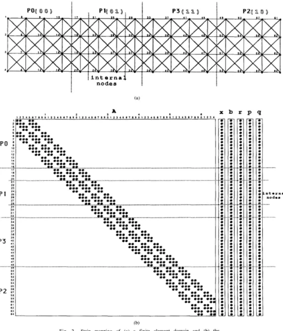
The communication considerations in distributing the CG
algorithm among the processors of a distributed-memory parallel computer may be understood with reference to Fig. 2. Fig. 2(b) displays the structure of a sparse matrix resulting from the finite element discretization of a simple rectangular region shown in Fig. 2(a). The discretization uses four-node rectilinear elements. In Fig. 2(a), the diagonals of the finite elements are joined by edges to give a finite element interaction graph, whose structure bears a direct relation to the zero-nonzero structure of the sparse system of equations that characterizes the discretization. Each node in a 2-D finite
1556
-
a 0 0 0 0 0 0 0 0 0 0 0 0 0 1. a 0 9. 0 0:
0 a .e. 0 e 0 9 . 0 0 0 0 0 a 0 0 0 0 0 0 a .&. 0 0 0 a 0 0 0 0 0 0 0 0 0 0 1IEEE TRANSACTIONS ON COMPUTERS, VOL 17. NO 12. DECEMBER 1YXX
. . . ... int.rn.1 n o d a s ... .. . ... . . ... .. . .... . ... i i n t e r n a j
i
nodes r D D D D 0 0 0 e 0 0 0 0 0 0 e. 0 08.
0 0 0 0 0 0. 0 0 Q. a a 0 0 0 0 a a 0 0 0 0 0 0 $., 0 0 D P D D D D D D D D L , x b - 0 0 0 0 0 0 0 0 0 0 0 0 0 e*
0 0 a 9. 0 0 0 0 0 0 ID. 0 0 0 Q. 0 0 0 0 0 0 0 0 0 0 0 0 a.i
0 0 0 0 0 0 0 0 0 0 0 0 4 e-
e = P 3 4 7 P 0:
10 1 1 I2 1 1 1. IS I7 I 8 I B ...!. q. ..f;, 2 2 23 P 12;
27 ..XP. 30 1 1 ... ? I . 1 4 35 30 37 31 39 P3::
,a .a..
l 6 .e 47 ... ;;. . 6 0 I1 S 2 53 6 4 5 s P 2%%
s9 8 0 I1 I2 63 a. 125410719~1~5460lI~~I25410719~12~~Ill19~1250I7~9~12~4I0719~~~~ 1 9 . 0. 2 6 0 0 0 0 0 0 0 0 0 0 0 0 0 0 0 I @ . 0 0 0 0 *eo. 0 0 0 0 0 0 0 0 0 00. 0 0 0 O**O*O..OO.. 0 0 0 0 0 0 0 0 0 0 0 0 0.0 0 0 0 00 aa ea 0 0 0 0 0 0 0 0 . 0 0 0 0 0 0 0 0 0 0 0 0 0 0 0 ... e.* ... a.e ... am ... ... 0. 0 0 0 0 0 0 0 0 0 0 0 0 0 0.0 0.0 0.0 ... @.Q.64@[email protected].~w ... .. .... . 0 0 0 0 0 0 0 0 0 0 0 0 0.0 0 0 0 em 0 0 0 0 00 0 0 0 0 0.0 0.0 0.0 0 0 0 0 0 . 0.0 sa ... as ... 0.a ... 0 0 0 0 0 0 0.6) 00. 0.0 ... 0 0 0 0 0 0 ..e ob ... RIT*l.R .... .*o.*&. ... 0 0 0 0.0 0.0 0 0 0 e00 0 0 0 0. 00 0. 0. 0 0 0 0 0.0 0.0 0.0 0 0 0 0 0 0 0 0 0 ea e m eo 0 0 ea me 0.0 0 0 0 0 0 0 0.0 0 0 0 .e0 0 0 0 0 0 0 0. 0 0 0. 0.0 0 0 0 0 0 0 0 0 0 reo 0 0 0 ... Rd***.*.&.0w6 . . . 0 0 0 0 0 0 0 8 0 0 0 0 0 0 0 0 0 0 0. 0 0 0 0 0 0 0 0 0 0 0 0 0 0 0 0 0 0 0 0 0 0 0 0 0 0.0 0 0 0 0 0 0 0. 0. 0 0 e a 0 0 a 0 eaa 0 0 0 0 0 0 e 0 0 0 0. 0 0 0 0 0 0 0 0 0 0 . 0 0 0 e a 0 0 0 (b)Fig. 2. Strip mapping of (a) a finite element domain and (b) the corresponding A matrix onto a 2-D hypercube.
element graph is associated with two variables, corresponding
to two degrees of freedom. Each nodal degree of freedom has
a corresponding row in the matrix A and is associated with a
component in the vectors x, b , r , p , and q . Furthermore, it can
be seen that the nonzeros in that row (column) of A occur only
in positions corresponding to finite element nodes directly
connected to that node in Fig. 2(a). The figure shows only a
single point corresponding to the two degrees of freedom of a
node. The matrix A and vectors x, b , r , p ? and q are shown
partitioned and assigned to the processors of a two-dimen-
sional hypercube. The partitioning of the matrix A and vectors
x, b , r , p , and q can equivalently (and more conveniently) be
viewed in terms of the partitioning of the corresponding nodes
of the finite element interaction graph itqelf. as shown in Fig. If the values of cyk and (Ik are known at all the processors,
the vector updates in steps 3, 4, and 6 of the CG algorithm can
clearly be performed very simply in a distributed fashion without requiring any interprocessor communication. The
individual pairwise multiplications for the dot products in
steps 2 and 5 can also be locally performed in each processor.
If each processor then forms a partial sum of the locally generated products, a global sum of the accumulated partial sums in each of the processors will result in the required dot
product. Considering the arithmetic computations required in
Steps 2-6, if the rows of A are evenly distributed among the 2(a).
AYKANAT et al.: ALGORITHMS FOR SOLUTION OF LINEAR EQUATIONS ON HYPERCUBES
1557
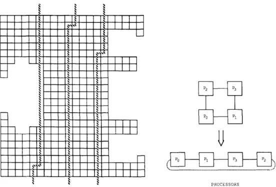
Fig. 3. Illustration of 1-D strip
U
PROCESSORS partitioning.
processors, each processor will perform exactly the same amount of computation per phase of the C G algorithm. Thus, with respect to Steps 2-6 of the algorithm, any balanced mapping of the finite element nodes among the processors is essentially equivalent in terms of the total amount of computa- tion and communication. This however is not the case as far as step 1 goes, as discussed below.
Step 1 of the algorithm requires a sparse matrix-vector
product. This involves the formation of the sparse dot product
of each row of A with the dense vector p , necessitating
interprocessor communication to obtain necessary nonlocal
components of the p vector. Due to the relation between the
nonzero structure of A and the interconnection structure of the
finite element interaction graph, the interprocessor communi- cation required is more easily seen from Fig. 2(a) than directly from Fig. 2(b)-two processors need to communicate if any node mapped onto one of them shares an edge with any node mapped onto the other. Thus, the interprocessor communica-
tion incurred with a given partitioning of the matrix A and the
vectors x, b , r, p , and q can be determined by looking at the
edges of the finite element interaction graph that go across
between processors. Therefore, in treating the partitioning of
the sparse matrix A for its efficient solution using a parallel
CG algorithm, in what follows, the structure of the finite element graph or associated finite element interaction graph is
referred to rather than the structure of the A matrix itself.
The time taken to perform an interprocessor communication on the Intel iPSC/2 system is the sum of two components-1) a
setup cost Sc that is relatively independent of the size of the
message transmitted, and 2) a transmission cost Tc that is
linearly proportional to the size of the message transmitted. Thus,
(3)
Tc,,,,,, =
sc
+
I x Tcwhere I is the number of words transmitted. The setup cost is
essentially independent of the distance of separation between the communicating processors, but is a nontrivial component of the total communication time unless the message is several thousand bytes long. Since an additional setup cost has to be paid for each processor communicated with, in attempting a mapping that minimizes communication costs, it is important to minimize not only the total number of bytes communicated, but also the number of distinct processors communicated with.
The first of the two mapping schemes described, the 1-D strip-
mapping approach [ 131, minimizes the number of processors
that each processor needs to communicate to, while simultane- ously keeping the volume of communication moderately low. The second scheme, the 2-D mapping approach [13], lowers the volume of communication, but requires more processor pairs to communicate. The two schemes are compared and it is shown that for the values of the communication parameters of
the Intel iPSC/2 and the range of problem sizes of current
interest, the 1-D strip mapping scheme is the more attractive one.
B.
1-D
Strip PartitioningThe I-D strip-mapping scheme attempts to partition the finite element graph into strips, in such a way that the nodes in any strip are connected to nodes only in the two neighbor strips. By assigning a strip partition to each processor, the maximum number of processors that any processor will need to communicate with is limited to two. The procedure can be understood with reference to Fig. 3. The finite element graph
shown has 400 nodes. A load-balanced mapping of the mesh
onto a two-dimensional hypercube with four nodes is therefore 100 nodes per processor. Starting at the top of the leftmost column of the mesh, nodes in that column are counted off,
1558 IEEE TRANSACTIONS ON COMPUTERS. VOL 17. NO I?. DECEMBER I Y X X
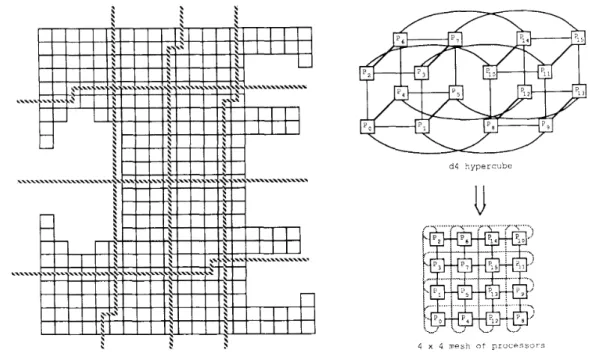
Fig 4 Illustrdtion of 2-D orthogonal
d4 5,ypercube
U
4 x 4 mesh of p r o c e s s o r s
strip partitioning. until 100 nodes are visited. Since the number of nodes in the
leftmost column is less than 100, the column immediately to its right is next visited, starting again at the top. By so scanning
columns from left to right, 100 nodes are picked off and
assigned to Po. Continuing similarly, another strip of 100
nodes is formed and assigned to P I . Pi and Pz, respectively, are assigned the next two such strips.
Thus, by only using a subset of the links of the hypercube, a linear chain of the processors is formed and adjacent strips generated by the strip mapping are allocated to adjacent processors in the linear chain. If the finite element mesh is
large enough, such a load-balanced 1-D strip mapping is
generally feasible. The scheme described above can be
extended to more general rectilinear finite element graphs that
cannot be embedded onto a regular grid; details may be found
in [13].
C. 2 - 0 Orthogonal Strip Partitioning
The partitions produced by 1-D strip mapping tend to
require a relatively high volume of communication between
processors due to the narrow but long shape of typical strips.
The 2-D orthogonal partitioning method attempts to create
partitions with a smaller number of boundary nodes, thereby reducing the volume of communication required. It involves the generation of two orthogonal 1-D strips. The hypercube
parallel computer is now viewed as a P I x P2 processor mesh.
A PI-way 1-D strip and a P2-way 1-D strip in the orthogonal
direction are generated, as illustrated in Fig. 4 for mapping the
mesh of Fig. 3 onto a 16-processor system. Partitions are now
formed from the intersection regions of the strips from the two orthogonal 1-D strips, and can be expected to be more “square” (and consequently have a lower perimeteriarea) than those generated by a 16-way 1-D strip mapping. It can be easily shown that the generated partition satisfies the “nearest
neighbor” property [13], i.e.. each such partition can have
connections to at most eight surrounding partitions. Further-
more, by using a synchronized communication strategy
between mesh-connected processors, whereby for each itera- tion, all processors first complete communications with horizontally connected processors before communicating with
their vertically connected processors, each processor needs to
perform at most four communications [ 131.
While each of the two orthogonal 1-D strip partitions is
clearly load balanced, the intersection partitions in Fig. 4 are definitely not. Such a load imbalance among the intersection partitions can in general be expected. Consequently, the 2-D strip partitioning approach employs a second boundary refine- ment phase following the initial generation of the 2-D orthogonal strip partition. The boundary refinement procedure
attempts to perform node transfers at the boundaries of
partitions in such a way that the nearest neighbor property of
the initial orthogonal partition is retained. The resulting
partition after boundary refinement for the chosen example
mesh is shown in Fig. 5. Details of the boundary refinement
procedure and generalization of the orthogonal 2-D mapping
procedure for nonmesh finite element graphs may be found in
~ 3 1 .
D. Comparison of I-D Versus 2 - 0 Partitioning
In this subsection, the 1-D and 2-D approaches are
compared with respect to the communication costs incurred
for the matrix-vector product of step 1 of the CG algorithm.
To facilitate a comparison, first a simple analysis is made for the case of a square mesh finite element graph with “in” nodes on a side. The communication costs with a I-D strip
partition and a 2-D partition are formulated. A special case of
2-D orthogonal strip partitioning, where a two-way partition is
1559
AYKANAT el al.: ALGORITHMS FOR SOLUTION OF LINEAR EQUATIONS ON HYPERCUBES
m
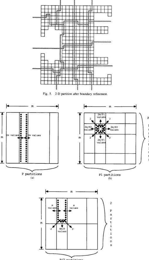
Fig. 5. 2-D partition after boundary refinement.
-m- m
1
2 P a r t i t i n 0 Sm
P P/2 partitions (C)Strip mapping of a regular m x m finite element mesh onto P
processors: (a) 1-D strip mapping, (b) 2-D strip mapping, ( c ) 1.5-D strip mapping.
1560 IEEE TRANSACTIONS ON COMPUTERS. VOL 3 7 , NO 12, DECEMBER IYR8
special case is interesting since it requires a maximum of three communications by any processor in any iteration, in contrast
to two and four, respectively, for the 1-D and general 2-D
case. Thus, the setup cost incurred with this special 2-D
mapping is in between that of the other two, and the
communication volume is also somewhere in between. This
special case of 2-D orthogonal partitioning is hence referred to
as a 1.5-D partition.
The load-balanced partitioning of an m
x
m node finiteelement mesh is shown in Fig. 6(a), (b), and (c) for the 1-D, 2- D, and 1.5-D cases, respectively. The use of a synchronized
interprocessor communication strategy alluded to earlier can
be used with the 2-D and 1.5-D cases. By performing all horizontal communications before vertical communications, the values to be transferred diagonally can be transmitted in a store-and-forward fashion, without incurring an additional setup cost for the diagonal communications. Thus, the number of transfers required between diagonally related processors in
the mesh is added on to the volume of the intermediate
processor’s communication. The number of variables is twice
the number of nodes in the sample finite element problems
used here. In the 2-D case then, each interior processor has an additional eight values added to its total communication
volume, corresponding to the four diagonal transfers from its
neighbors that it facilitates through a store-and-forward transmission. By referring to Fig. 6(a), (b), and (c), it is easy
to see that communication times T I D , T2D, and TI.,, for 1-D, 2-D, and 1.5-D strip mapping, respectively, can be expressed as
T l D = 2 x S C + 4 m x T, (4)
( 5 )
( 6 ) The relative merit of one scheme over the other is a function
T~LI = 4 X SC+ (8 + 4 m / P l
+
4m/P2) T, P , , Pz> 2T , ,511 = 3 x SC
+
(4+
2m t 4 m / P ) T,. of P , SC, and T,, and m as followsFrom these inequalities, it is concluded that for P = 16, P I =
P 2 =
6
= 4 the optimal approach is 1-D strip partitioning,i
for m < ? x 8 ( % + 2 )I
1.5-D strip partitioning, I1
2-D strip partitioning, LThe above simplified analysis precludes the possibility of overlap between multiple out-bound communications from a processor. While such overlap is possible, the setup times for the individual communications are truly additive and cannot be
overlapped. A more detailed analysis assuming overlap
between the transmission times with succeeding setup times provides results similar to the above simplified analysis with
respect to the ranges of m where each of the above schemes is
optimal.
Using experimentally measured values for Sc = 970 ps and
Tc = 2.88 ps per double-precision number, it is seen that the
1-D approach is superior to the other two for m
<
194. Thisvalue of m is well above mesh sizes of interest in the context of
a practically realistic finite element solution. While the above analysis considered a specific shape of a finite element graph, it provides a good estimate of the order of magnitude of the finite element graph size that makes the 1.5-D or 2-D
approaches worth using for a parallel finite element solver on
the Intel iPSC/2. Table I summarizes the results obtained with
1
1 TI .5
<
T2 iff m<
(
+
2)x
(1 + 2 / P - 2 / P , - 2 / P , ) For the case of a 16-processor hypercube system, we obtain
P = 1 6 , P l = P 2 = J 1 6 = 4
(7)
~ ~ _ _ _ __ _ ~ _ _ ~- ~ ~ ~~~ ~
a number of finite element graphs using the three approaches. The total volume of communication required by the partition with the largest boundary is reported, as well as the predicted
communication time for the local communication phase in
each case. It can be seen that for every one of the examples,
the partitions produced by the 1-D approach are clearly
superior. As a consequence, only the communication protocol
required by 1-D strip partitions was actually implemented on
the Intel iPSC/2 system for the parallel CG algorithm. The
formulation, implementation, and experimental performance
measurement of the parallel CG algorithm are treated in the
AYKANAT et al.: ALGORITHMS FOR SOLUTION OF LINEAR EQUATIONS ON HYPERCUBES 1561
Sample Problem
Yo. Mesh Mesh No. of
Size Description Nodes
T1 15 x 20 Rectanaular 300
Max. Communication Est. Communication Volume in DP words
I-D
I
1.5-DI
2-D 1-DI
1.5-DI
2-D 64 I 46 I 48 2124 I 3042 1 4018Time in jisecs
IV. FORMULATION OF A COARSE GRAIN PARALLEL SCG
(CG-SCG) ALGORITHM
Strong data dependencies exist in the basic SCG algorithm which limit the available concurrency. The distributed inner
product computation ( P k , q k ) which is required for the
computation of the global scalar f f k cannot be initiated until the
global scalar b k - 1 is computed. Similarly, the inner product
( r k + [ , r k + I ) which is required for the computation of the
global scalar b k cannot be computed until the global scalar f f k
is computed. During each SCG iteration, three distributed vector updates which involve no communication and one matrix-vector product which involves only local communica- tion cannot be initiated until the updating of these global scalars is completed. Hence, these data dependencies due to the inner product computations introduce a fine grain parallel-
ism which degrades the performance of the algorithm on the
hypercube.
The SCG algorithm requires the computation of two inner product terms at each iteration step. These inner product calculations require global information and thus are inherently sequential. The Global Sum (GS) and Global Broadcast (GB)
operations [7] both require
d
communication steps andintroduce a large amount of interprocessor communication overhead, due to the large setup time for communication. Furthermore, only one floating point word is transferred and one inner product term is accumulated during the GS-GB communication steps due to the data dependencies in inner
product computations. New formulations of the SCG al-
gorithm that allow the parallel computation of the inner products are discussed in [ l o ] and [14]. The formulation described in [lo] is used here with a different motive, namely to reduce the number of setups for communication. This coarse grain SCG algorithm enables the computation of two inner products in one GS-GB step as described in the next section. Further improvement is obtained by using a global sum algorithm that takes advantage of the two physical links between connected processors, in the architecture, to overlap communication in two directions.
A . CG-SCG
f o r s
= IThe rationale behind this formulation is to rearrange the
computational steps so that two inner products can be
communicated in each GS-GB communication step after
computing the distributed sparse matrix-vector product q k =
A p k . The problem is to find the expressions for the global scalars f f k and @ k in terms of these inner products. Using the recurrence relation given in Step 3 of the SCG algorithm, we
have
Using the recurrence relation defined for r k + once more,
( r k + l , A p k ) = ( r k , A p k ) - a k ( A p k , A p k ) (11)
is obtained. Now using the recurrence relation defined for P k
in step 6 of the SCG algorithm,
( r k , A p k ) = ( p k , A p k ) - @ k - I ( P k , A P k - l ) = ( p k , A p k ) (12) is obtained. Note that ( P k , A p k - , ) = 0 since the direction
vectors generated during the SCG algorithm are A orthogonal
[ l l ] . Hence, inserting (12) into (11) and then (11) into (10) one can obtain
- 1. ( P k , A p k ) - f f k ( A p k , A p k ) ( A p k , A p k )
b k = - = f f k
( P k , A p k ) ( P k 9 A p k ) Therefore, the inner products ( P k , A p k ) and ( A p k , A p k ) are
needed to compute the global scalars f f k and @ k . The value of
the inner product ( r k + l , r k + l ) which is required for the
computation of the global scalar f f k + on the next iteration can
be computed in terms of the previous inner product ( r k , r k ) using
( r k + l , r k + l ) = @ k ( r k , r k ) . (13)
The initial inner product (ro, ro) is computed using the GS-GB
algorithm. Hence, the steps of the coarse grain parallel SCG algorithm can be given as follows.
Choose XO, let ro = PO = b - A x 0 and compute (ro,
ro).
Then, for
k
= 0, 1, 2,1. form q k = A p k
2. a) form ( P k , q k ) and ( q k , q k ) (in one GS-GB communi- cation step) 3. a) a k = ( r k , r k ) / ( P k , q k ) b) b k = ( a k ( q k , q k ) / ( P k , q k ) ) - 1.
cl
( r k + l , r k + l ) = b k ( r k , r k ) 4. r k + l = r k - a k q k x k + l = x k + a k P k P k + l = r k + l+
b k p k .1562 IEEE TRANSACTIONS ON COMPUTERS, VOL. 37. NO I ? , DECEMBER 19x8
TABLE I1
SOLUTION TIMES (PER ITERATION) FOR B - S C G AND CG-SCG AL- GORITHMS ON i P S C 2 i d 4 HYPERCUBE FOR DIFFERENT SIZE FINITE
ELEMENT PROBLEMS
N o No. t P S C 2 l d l iPSCZld2 tPSCZld3 iPSCZld4 Test
11
Mesh'
of1
of1'
sol. time((
sol. timeI/
sol. time//
sol. timeI/
T7
11
49 x 49 147521
297 11 -1
-11
- I - /I 215.3 I 210.2 11 116.1 1 110.8 11from two to one per iteration of the SCG algorithm. Note that the volume of communication does not change when compared to the basic SCG (B-SCG) algorithm, since two inner product values are accumulated in a single GS-GB communication step. The computational overhead per iteration is only two scalar multiplications and one scalar subtraction which is
negligible. The number of divisions is reduced from two to
one ( l / ( p k , q k ) is computed once).
Numerical results for a wide range of sample problems show that the proposed algorithm introduces no numerical instability and it requires exactly the same number of iterations to converge as the (B-SCG) algorithm. The solution times of different size sample finite element problems for B-SCG and
the CG-SCG algorithms, on 1 -4-dimensional iPSC/2 hyper-
cubes, are given in Table 11.
B . CG-SCG f o r s = 2
The rationale behind this formulation is to accumulate four and ( A ' P z k , A 2 p 2 k ) in a single GS-GB communication step after computing two consecutive distributed matrix-vector products 4 2 k = A p 2 , and U2k = A q 2 k and then compute four global scalars a Z k ,
PZk,
a 2 k + I , andPZk+
The derivation of the expressions for these global scalars are too cumbersome andhence are omitted here. The basic steps of the algorithm for s
= 2 are given below.
inner products ( P Z k , A p 2 k ) > ( A P Z k , A p 2 k ) > ( A p 2 k 9 A 2 P 2 k ) ,
Choose X O , let
P -
I = 0 , 4 - I = 0, and then compute ro = p o = b - Axo and Then, for d) a Z k + l = (11 - a 2 k 1 2 ) / ( 4 2 - a z k l 3 )+
0 2 k 1 2 e) 63 = 13+
0 2 k - l / a 2 k - 1 ( $ 2+
1 / a 2 k - I 1 1 ) f ) 0 2 k + l = 8) ( r 2 k + l , r 2 k + l ) = 0 2 k @ Z k + l (TZk, r2k) b) P 2 k + 1 = r 2 k t 1 -k P 2 k P 2 k c) X Z k + 2 = X2k+
a 2 k P 2 k+
a 2 k + l P Z k + l d) A P x + I = - 0 2 k - 1 A p 2 k - 1+
(1 f 0 2 k ) A P Z k - - a 2 k + 1 [ ( ' $ 2 - a 2 k 1 3 ) - aYZkil(43+
P2k13 - a Z k 1 4 ) 1 / ( 4 - a 2 k l 2 ) 4. a) r 2 k + l = r 2 k - a 2 k A P 2 k a 2 k A 'P 2 k e) r 2 k + 2 = r 2 k t - l - a Z k + l A P Z k + l f ) P 2 k + 2 = r Z k + 2+
0 2 k + l P 2 k + l .Note the one iteration of the above algorithm corresponds to two iterations of the basic SCG algorithm. Hence, the number of global communication steps is reduced by a factor of four, that is, from twice per iteration to once every two iterations. The scalar computational overhead of this algorithm is 12
multiplications and IO additiodsubtractions per SCG itera-
tion which can be neglected for sufficiently large n, where n
= N / P . However, there is also a single vector update overhead per SCG iteration, giving a percent computational overhead of 2:(1
/ ( z
+
5 ) ) 100 percent, wherez
is the averagenumber of nonzero entries per row of the A matrix. For z =
18, where each node interacts with eight other nodes and there
are two degrees of freedom per F E node, the overhead is
2: 4.4 percent. Hence, this algorithm is recommended only for
solving sparse linear systems of equations with A matrices
having large
z ,
on large dimensional hypercubes. Thisapproach can be generalized for larger s values. However, the
computational overhead increases with increasing s and
furthermore the numerical stability of the algorithm decreases with increasing s.
C. Comparison of B-SCG and CG-SCG
The solution times of B-SCG and the CG-SCG (for s = 1 )
algorithms for different size test FE problems on a four-
dimensional hypercube, iPSC/2, are given in Table 11. The
percentage performance improvement, 7 = [( T B s C C -
T c ~ s c c ) / T c ~ s c c ] * 100 percent, decreases with the increasing
problem size, since the ratio of the GS-GB communication time to the total solution time per iteration decreases by
increasing problem size. Here, TBscG denotes the time taken
by the B-SCG algorithm and TccscG denotes the time taken by
AYKANAT ef al.: ALGORITHMS FOR SOLUTION OF LINEAR EQUATIONS ON HYPERCUBES
_____
1563
hypercube (iPSC2/d4), 7 monotonically decreases from 24
percent for the smallest test problem T1 to 5 percent for the
largest test problem T 7 . It can be also observed from Table I1
that 7 increases with the increasing dimension of the hyper-
cube, since the complexity of the GS-GB algorithm increases linearly with the dimension whereas the granularity of a problem decreases exponentially with the dimension, as the domain is divided among 2 d processors. For example, for the
smallest size test problem T 1, 7 increases monotonically from
2 percent on iPSC2idl to 24 percent on iPSC2id4. Hence, the
proposed CG-SCG algorithm is expected to result in signifi- cant performance improvement on large dimensional hyper- cubes.
D.
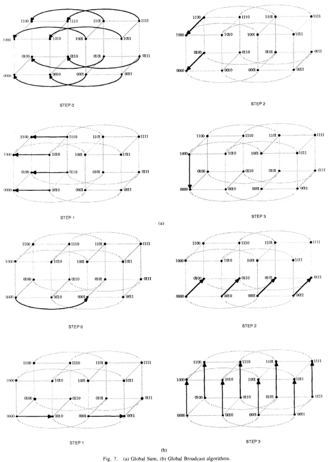
The Exchange-Add AlgorithmAs already mentioned, to compute the inner products in step 2 of the CG-SCG algorithm, the partial sums computed by
each processor must be added to form the global sums ( ( p k ,
q k ) and ( q k , q k ) ) . Furthermore, since these values are needed in the next step by all processors, they must be distributed to all processors. The global sum algorithm [7], shown in Fig.
7(a), for a d = 4 dimensional hypercube requires d nearest
neighbor communication steps. The computations and nearest neighbor communications (shown by solid lines) at the same step of the algorithm are performed concurrently.
The global broadcast algorithm [15], shown in Fig. 7(b), for
a d = 4 dimensionzL hypercube also requires d nearest
neighbor communication steps. Hence, a total of 2 d concur- rent nearest neighbor communication steps are required. Note that most of the processors stay idle during the global sum and
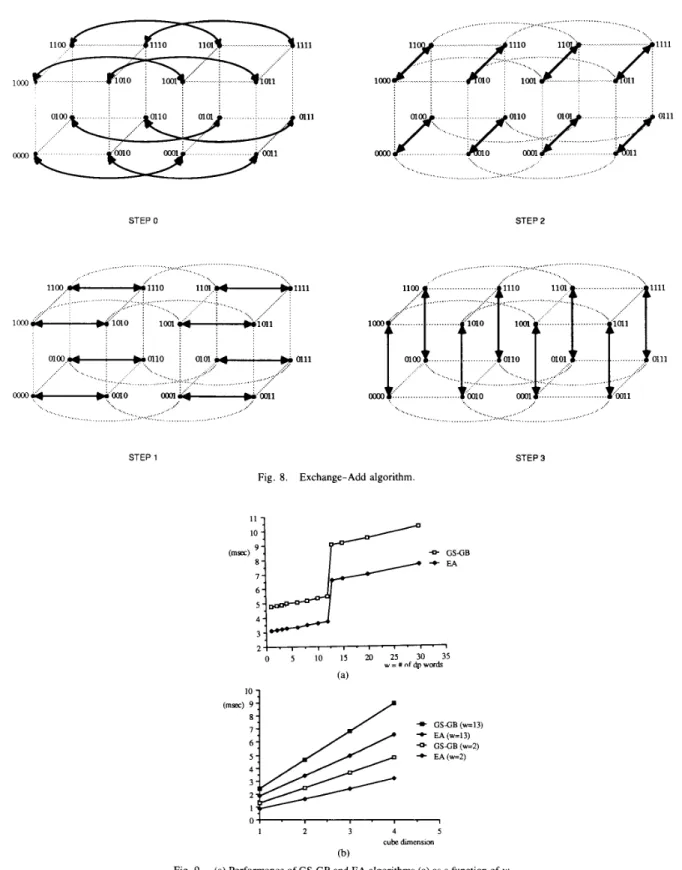
global broadcast steps. An alternative algorithm, the Ex-
change-Add algorithm is illustrated in Fig. 8. The main idea
in this algorithm is that each processor accumulates its own copy of the inner product instead of only one processor accumulating it and then broadcasting. Let the processors of a d-dimensional hypercube be represented by a d-bit binary
number
(zd-
* a , zo). Also, define channel i as the set of(2d- ’) bidirectional communication links connecting two
neighbor processors whose representation only differs in bit
position i . Then, the steps of the Exchange-Add algorithm
can be given as follows.
Initially, each processor has its own partial sum. step i : f o r i = 0 , a . . , d - 1
1. processors P ( z d - I ,
. .
e ,z,+
0, zr- ],. .
,
z o )
and P(zd-1, * ..,
z,+1,
1,z , - ] ,
e-.,zo)
concurrentlyexchange their most recent partial sums over channel i.
2. each processor computes its new partial sum by adding
~~ ~
if
else
end
the partial sum it received over channel i to its most
recent partial sum.
This algorithm requires d exchange steps that can be over-
lapped when two physical links are present. At the end of d
exchange steps, each processor has its own copy of the sum. Fig. 9(a) and (b) illustrates the performance of the GS-GB and E A algorithms with respect to the number of double-
precision ( D P ) words (w) added and the dimension of the
hypercube, respectively. The node executive (NX/2) of the
iPSC/2 handles short messages (I 100 bytes) and long
messages (> 100 bytes) differently. Short messages are routed
directly, whereas extra handshaking is performed between the two processors participating in the communication to establish the circuit for the transmission of a large message. This extra
overhead causes the setup time to increase from Sc = 550 ps
to Sc = 970 p s for long messages. This explains the jumps in
the curves given in Fig. 9(a) at w = 13 (104 bytes). The
measured performance for the GS-GB is found to be within 5
percent of the estimated lower bound, TZ’GB = d [ 2 ( S c
+
wT,)
+
wTcalc], where T,,,, is the time taken for a single D P add operation. However, the measured performance of the E A algorithm varies from T Z a S = 1.3 TF$ (for w = 1 ) to TEas =1.6TE$ (for w = 30), where T,“,:‘ = d [ ( &
+
W T C )+
w Tcalc] (TE: = 1 /2
y2-GB
for small w). This discrepancy canbe attributed to the software overheads for short messages and internal bus conflicts for long messages.
E. Implementation of the Parallel CG-SCG Algorithm
The distributed computations of the CG-SCG algorithm consist of the following operations performed at each iteration:
matrix-vector product q k = A p , (Step I), inner products (pk,
4,) and ( q k , q k ) (Step 2), and the three vector updates required in Step 4. All of these basic operations are performed
concurrently by distributing the rows of A , and the corres-
ponding elements of the vectors b , x, r , p , and q among the
processors of the Intel iPSC/2 16-node hypercube. Each
processor is responsible for updating the values of those
elements of the vectors x, r , p , and q assigned to itself. The 1- D approach has been implemented to distribute the problem due to its superior features for iPSC/2 as discussed earlier. In this scheme, all but the first and the last processors in the linear array have to communicate with their right and left neighbors at each iteration in order to update their own slice of
the distributed q vector. The following communication topol-
ogy is implemented to utilize the two serial bidirectional communication channels between the processors for overlap- ping these nearest neighbor communications.
my processor number has even parity in the Gray code ordering then
receive p i E {my right neighbor’s left boundary} from my right neighbor send p i E {my right boundary} to my right neighbor
receive p i E {my left neighbor’s right boundary} from my left neighbor send p i E {my left boundary} to my left neighbor
if my processor number has odd parity in the Gray code ordering then
receive p i E {my left neighbor’s right boundary} from my left neighbor send p i E {my left boundary} to my left neighbor
receive p i E {my right neighbor’s left boundary) from my right neighbor send p i E {my right boundary} to my right neighbor
1564 IEEE TRANSACTIONS ON COMPUTERS. V O L 37, NO I ? . 1)ECEMHkK I Y X X STEP 0 STEP 1 STEP 0 1100 ........................... ,1110 11m.e ... ill11 1100 0 ,1110 i i m e1111 100. 41010 1001e 01011 moo 0111 Ocnl .ono m o l 0 0111 mx, a0010 0001. STEP 2 STEP 3 STEP 2 STEP 1 STEP 3 (b)
1565 AYKANAT er al.: ALGORITHMS FOR SOLUTION OF LINEAR EQUATIONS ON HYPERCUBES
1111 0111 m STEP 0 1111 :011o j a o l k j k ' 0111 : ~ 0 0 . ~ i b ... . . . , ,/.. . . . : .. .. .., ' : .:? m STEP 1 ... ... ... ...:. ... .... . . ' /.:. ... ... : .: .... ... I ... ... /In1 . . . ./. 0111 ... ... ... ..:.' 0 ... STEP 2 ... ... ... : .... ... ... .... ... , .. , .... ... ... '. ... STEP 3 Fig. 8. Exchange-Add algorithm.
GSGB + E A o 5 10 15 20 25 30 35 w =
*
nf dp work (a)*
GSGB(w=13) + EA(w=13) -a- G S G B ( w 2 ) + E A ( w 2 )" .
1 2 3 4 5 cute dunension (b)(b) as a function of cube dimension.
1566 IEEE TRANSACTIONS ON COMPUI'ERS. VOL 37. N O I 2 DFCFMBkR 198X
T A B L E 111
SOLUTION TIMES (PER ITERATION) FOR B SCG WITH GS-GB ALGORITHM AlvD C G S C G WITH EA ALGORITHM ON 1 P S C 2 i d 4 HYPERCUBE FOR
DIFFERFNT S17E FINITE ELEMENT PROBLEMS
A lower bound for the complexity of this local communica-
tion step is T,,,,,,, = 2(Sc
+
2mTc), which holds underperfect load-balanced conditions, i.e.,
nk
= N / P variablesmapped to each processor and each processor has an equal
number o f F E nodes at its right and left boundaries. Each
processor of a pair coupled to communicate with each other issues a nonblocking (asynchronous) send after issuing a
nonblocking receive. This is done to ensure that a receive is
already pending for the incoming long message so that it can
be directly copied into the user buffer area instead of being
copied to the N X I 2 area and then transferred to the indicated
user buffer due to a late issued receive.
The F E nodes mapped to a processor can be grouped as
infernaf nodes and boundary nodes [Fig. 2(a)]. Internal
nodes are not connected to any F E nodes mapped to another
processor and boundary nodes are connected to at least one
F E node which is mapped to a neighbor processor. The internal sparse matrix-vector product required for updating
the elements of the vector q h corresponding to the internal F E
nodes, does not require any elements of the vector
Pk
whichare mapped to the neighbor processors. Hence, the internal
sparse matrix-vector product computation on each processor is initiated following the asynchronous local communication steps given above. Each processor can initiate the sparse
matrix-vector product corresponding to its boundary F E
nodes only after the two receive operations from its two neighbors are completed. Note that the synchronization on the asynchronous send operations can be delayed until the distributed vector update operations at Step 4 of the CG-SCG algorithm. This scheme is chosen to overlap the communica- tion and the computation during the internal sparse matrix- vector product. However, the percent overlap is measured to
be below 5 percent due to the internal architecture o f
processors of the iPSCI2.
The EA algorithm described in the previous section is implemented to compute the two inner products in Step 2 of the CG-SCG algorithm. The volume of communication during
the d concurrent nearest neighbor communication steps of the
algorithm is only 16 bytes ( 2 DP words). The short messages
are always stored first into the N X I 2 buffer regardless of a
pending receive message. Hence. in the implementation of the
E A algorithm on the iPSCI2. each processor of a pair participating in the exchange operation issues a nonblocking send operation before the blocking receive operation in order to prevent the delay of the send operation. The updating of the two partial sums is delayed until the completion of the send operation.
Each processor of the hypercube computes its own copies of
the global scalars CY and in Step 3 of the algorithm in terms of
the two inner products computed in Step 2 of the CG-SCG algorithm. Then, at Step 4 of the algorithm. each processor updates its own slices of the distributed x, r , and p vectors, without any interprocessor communication using these global scalars. Solution times for this implementation are given in Table 111.
V. PERFORMANCE RESULTS A N I ) DISCUSSION
This section presents overall performance results for the parallel CG-SCG algorithm. A simple model can be used to
estimate an upper bound on achievable speedup. Given a 1 -D
strip partitioning of a finite clement graph onto P processors
so that Nk is the number of nodes mapped onto processor ph
and V k is the number of values to be communicated by /'A, the
iteration step time may be estimated as
where T,, =
( z
f 5)TCiglc is the execution time required foreach locally mapped variable, Sc and T(- are the setup time and
per value transmission time, and T:: is the global sum
evaluation time using the Exchange-Add algorithm. e is the
efficiency of the parallel implementation (spcedupIP). Since the iterations of the algorithm are synchronized, the bottleneck processor is the one with maximal sum of local execution cost
(2. T,;Nk) and communication cost (T(..
vh),
where the localcommunication cost is modeled as described earlier in Section
1567 AYKANAT et al.: ALGORITHMS FOR SOLUTION OF LINEAR EQUATIONS ON HYPERCUBES
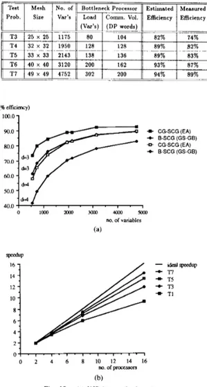
Test
Prob.
Mesh No. of Bottleneck Processor Estimated Measured
Size Var’s Load
I
Comm. Vol. Efficiency EfficiencyT 3 25 x 25 1175 80 (W elfcimcy) 100.0 1 104 82% 14% 60.01 w
f
f
T4 32 x 32 -- T5 33 x 33 T6 40 x 40 T7 49 x 49 40.0 50.0 { wf
, , ,.
,.
, ,,
1950 128 ~~ 128 89% ~ _ _ _ 82% -. 2143 138 136 89% 83% 3120 200 162 93% 87% 4752 302 200 94% 89% 0 I m o m m 4 a o m no. of variables (a) 4 CG-SCG(EA) + E-SCG (GS-GB) 0 CG-SCG(EA) + E-SCG (GS-GB) speedup 16 1 14 - 12-
IO-
8 - 6 - 4 - 2 - 0 2 4 6 E IO 12 14 16 110. of processors (b)Fig. 10. (a) Efficiency. (b) Speedup.
the time required to perform a global sum operation is added to
estimate the time for an iteration step. Table IV presents the
estimated processor efficiency for each of the sample problems and compares it to the experimentally measured efficiency on
the 16-node iPSC/2. The realized efficiency is within 10
percent of the upper bound for the large problems. The deviation from the estimated bound is due partly to the fact that the communication model used is overly optimistic in assum- ing that complete overlap of data transmission during simulta-
neous send/receive is possible. In practice, contention for an
internal bus for long messages during local communication steps results in a lower achieved transmission rate. Fig. 10(a) shows the percent efficiency as a function of problem size, for
d = 3 and d = 4. It can be seen that the CG-SCG algorithm
with EA is more efficient for cases where the amount of
computation per processor is smaller. Fig. 10(b) shows speedup as a function of the number of processors. It can be
seen that the implementation of the algorithm is scalable and an almost linear speedup is achieved for larger problems.
VI. CONCLUSION
Coarse grain algorithms for message passing hypercube multiprocessors were presented. The implementation on a 16-
node Intel hypercube of the (s = 1) algorithm and experimen-
tal results were discussed. The algorithm, as expected, results in a higher performance improvement for cases in which the partitioning of the domain results in fine grain computations
(small problems or large problems on large hypercubes) and
for large dimensional hypercubes as the communication overhead is a function of d, independent of the problem size.
The parallel CG-SCG algorithm is part of a finite element
modeling system (ALPID) for metal deformation, based on a
viscoplastic formulation. The incorporation of a parallel iterative solver in place of the original direct solver has made its effective parallelization on a hypercube parallel computer feasible.
ACKNOWLEDGMENT
We would like to thank S . Martin, S . Doraivelu, and H .
Gegel for helpful discussions and for their support and encouragement. We would also like to thank the anonymous referees for their valuable comments.
REFERENCES
G. A. Lyzenga, A. Raefsky, and G . H. Hager, “Finite elements and the method of conjugate gradients on a concurrent processor,” in Proc. ASME Int. Conf. Comput. Eng., 1985, pp. 393-399.
C. L. Seitz, “The cosmic cube,” Commun. ACM, vol. 28, pp. 22- 23, Jan. 1985.
J. M. Ortega and R. G. Voigt, “Solution of partial differential equations on vector and parallel computers,” SIAMRev., vol. 27, pp.
149-240, 1985.
R. Lucas, T. Blank, and J . Tiemann, “A parallel solution method for large sparse systems of equations,” IEEE Trans. Computer-Aided Design, vol. CAD-6, pp. 981-990, Nov. 1987.
H. Jordan, “A special purpose architecture for finite element analy- sis,” in Proc. IEEE I n t . Conf. Parallel Processing, Aug. 1978, pp. 263-266.
J. A. George and J. Liu, Computer Solution of Large Sparse Positive Definite Systems. Englewood Cliffs, NJ: Prentice-Hall,
1981.
J. P. Hayes, T . Mudge, Q. F. Stout, S . Colley, and J . Palmer, “A microprocessor-based hypercube supercomputer,” IEEE Micro, vol. 6, no. 5, pp. 6-17, 1986.
S . H. Bokhari, “On the mapping problem,” IEEE Trans. Comput.,
vol. C-30, pp. 207-214, Mar. 1981.
Z. Cvetanovic, “The effects of problem partitioning, allocation and granularity on the performance of multiple processors,” IEEE Trans. Comput., vol. C-36, pp. 421-432, 1987.
Y. Saad, “Practical use of polynomial preconditionings for the conjugate gradient method,” SIAM J . Scienti$ Statist. Comput.,
D. Luenberger, Introduction to Linear and Nonlinear Program- ming. Reading, MA: Addison-Wesley, 1973.
A. Jennings and C . Malek, “The solution of sparse linear equations by the conjugate gradient method,” Int. J . Numer. Meth. Eng., vol. 12, P. Sadayappan and F. Ercal, “Nearest-neighbor mapping of finite element graphs onto processor meshes,” IEEE Trans. Comput., vol. C-36, pp. 1408-1424, Dec. 1987.
G. Meurant, “Multitasking the conjugate gradient method on the CRAY X-MPl48,” Parallel Comput., no. 5, pp. 267-280, 1987. C. Moler, “Matrix computations on distributed memory multiproces- sors,” in Proc. SIAM First Conf. Hypercube Multiprocessors,
1986, pp. 181-195.
vol. 6, pp. 865-881, Oct. 1985.
1568 IEEE TRANSACTIONS ON COMPUTERS, VOL. 31, NO. 12, DECEMBER 1988 Cevdet Aykanat received the M.S. degree from
Middle East Technical University, Ankara, Turkey, in 1980 and the Ph.D. degree from The Ohio State University, Columbus, in 1988, both in electrical engineering.
From 1977 to 1982, he served as a Teaching Assistant in the Department of Electrical Engineer- ing, Middle East Technical University. He was a Fulbright scholar during his Ph.D. studies. Cur- rently, he is an Assistant Professor at Bilkent University, Ankara, Turkey. His research interests
Fikret Ercal (S’85) was born in Konya, Turkey. He received the B.S. (with highest honors) and M.S. degrees in electronics and communication engineer- ing from the Technical University of Istanbul, Istanbul, Turkey, in 1979 and 1981, respectively, and the Ph.D. degree in computer and information science from The Ohio State University, Columbus, in 1988.
From 1979 to 1982, he served as a Teaching and Research Assistant in the Department of Electrical Engineering, Technical University of Istanbul. He include supercomputer architectures, parallel processing, and fault-tolerant
computing.
has been a scholar of the Turkish Scientific and Technical Research Council since 1971. Currently, he is an Assistant Professor at Bilkent University, Ankara, Turkey. His research interests include parallel computer architec- tures, algorithms, and parallel and distributed computing systems.
Dr. Ercal is a member of Phi Kappa Phi. Fiisun Ozgiiner (M’75) received the M.S. degree
in electrical engineering from the Technical Univer- sity of Istanbul, Istanbul, Turkey, in 1972, and the Ph.D. degree in electrical engineering from the University of Illinois, Urbana-Champaign, in 1975. She worked at the IBM T. J. Watson Research Center for one year and joined the faculty at the Department of Electrical Engineering, Technical University of Istanbul. She spent the summers of 1977 and 1985 at the IBM T. J. Watson Research Center and was a visiting Assistant Professor at the University of Toronto in 1980. Since January 1981 she has been with the Department of Electrical Engineering, The Ohio State University, Columbus, where she presently is an Associate Professor. Her research interests include fault-tolerant computing, parallel computer architecture, and parallel al- gorithms.
Ponnuswamy Sadayappan (M’84) received the B.Tech. degree from the Indian Institute of Tech- nology, Madras, and the M.S. and Ph.D. degrees from the State University of New York at Stony Brook, all in electrical engineering.
Since 1983 he has been an Assistant Professor with the Department of Computer and Information Science, The Ohio State University, Columbus. His research interests include parallel computer archi- tecture, parallel algorithms, and applied parallel computing.