Interpolation techniques to improve the accuracy of the plane wave excitations in the finite difference time domain method

(1)

Radio Science, Volume 32, Number 6, Pages 218%2199, November-December 1997

Interpolation techniques to improve the accuracy

of the plane wave excitations in the finite

difference

time

domain

method

U•ur O•uz and Levent Giirel

Department of Electrical and Electronics Engineering, Bilkent University, Ankara, Turkey

Abstract. The importance of matching the phase velocity of the incident plane wave to the

numerical phase velocity imposed by the numerical dispersion of the three-dimensional (3-D) finite difference time domain (FDTD) grid is demonstrated. In separate-field formulation

of the FDTD method, a plane wave may be introduced to the 3-D computational domain

either by evaluating closed-form incident-field expressions or by interpolating from a 1-D

incident-field array (IFA), which is a 1-D FDTD grid simulating the propagation of the

plane wave. The relative accuracies and efficiencies of these two excitation schemes are compared, and it has been shown that higher-order interpolation techniques can be used to improve the accuracy of the IFA scheme, which is already quite efficient.

1. Introduction

The finite difference time domain (FDTD) method

was suggested three decades ago as a numerical tech-

nique to solve time-dependent Maxwell's equations

[Yee, 1966], whose general solution could not be ob-

tained otherwise. With the increase of computing power available to the scientists in recent years and

owing to the efficiency, flexibility, and the ease of im-

plementation of the FDTD method, it has become one of the most popular solution techniques in the area of computational electromagnetics.

New extensions and enhancements of the FDTD

method are continuously being introduced in order to employ the technique in the solution of new prob-

lems [Taftore, 1988; Taftore and Umashankar, 1989;

Kunz and Luebbers, 1993; Taftore, 1995; Shlager

and Schneider, 1995], perhaps as never envisaged

by the original developers. Electromagnetic scatter- ing problems, where the objects are placed in un- bounded media and illuminated by plane waves, are also among the wide variety of problems solved by using the FDTD method. The FDTD method does not automatically incorporate the radiation bound-

Paper number 97RS02515.

0048-6604 / 9 7 / 97RS- 02515511.00

ary condition; therefore it is more suitable for the solution of problems involving geometries enclosed in conducting or otherwise impenetrable boxes, such

as closed waveguides, shielded microwave integrated

circuits (MICs) and cavities [DePourcq, 1985]. How-

ever, due to the importance of the scattering prob- lems in the computational electromagnetics, they were the first problems to be solved using the FDTD

method [Yee, 1966], even before the concept of

absorbing boundary conditions (ABCs) was intro- duced. Later on, the development of the early ABCs

[Merewether, 1971; Lindman, 1975] and the solu- tion of scattering problems [Taftore and Brodwin, 1975; Mur, 1981] progressed hand in hand.

Although the FDTD method was originally devel-

oped [Yee, 1966] as a "time domain" method and

other electromagnetic solution techniques exist for

"frequency domain" problems [Harrington, 1982; Miller et al., 1992], the FDTD method is frequently

employed in obtaining the sinusoidal steady state so-

lutions of complicated electromagnetics problems ex-

cited with time-harmonic sources [Taftore and Brod-

win, 1975; Taftore, 1980; Mur, 1981; Umashankar and Taftore, 1982; Taftore and Umashankar, 1983;

Tafiove et al., 1985]. This is mainly due to the sim-

plicity of the FDTD method and its ability to model

complicated inhomogeneities with ease and at no ex-

tra cost. Sinusoidal excitation within the FDTD

method is used even for some problems that need to

(2)

2190 O•UZ AND GOREL' IMPROVING ACCURACY OF PLANE WAVE EXCITATIONS

be solved over a finite frequency band. An example

is the computation of the radar cross section (RCS)

of an object at multiple frequencies.

Being a computational method, the FDTD method

produces results with finite accuracy. If this accu-

racy is sufficient for a given application, the results are considered to be reliable. In the past, 1-2 dB of accuracy was targeted with the FDTD method

[Tafiove, 1980; Tafiove et al., 1985], and this accu-

racy was sufficient for the engineering applications considered at that time. Noting that 1-dB accuracy

corresponds to 12% error in the signal and 26% error

in the power, we can conclude that the range of ap- plications, where this much error is still acceptable, is getting narrower. Recently, FDTD solutions with subdecibel accuracy have become possible due to the progress in the following areas:

1. More accurate ABCs have been developed to reduce the reflection error while keeping the problem

size at reasonable levels [B•renger, 1994, 1996a, b].

2. High-performance computers have become avail-

able. Hence larger problems corresponding to denser

FDTD meshes and higher-order FDTD algorithms

[Fang, 1989; Deveze et al., 1992; Omick and Castillo, 1993; Manry et al., 1995] can be solved to reduce

the dispersion error due to the coarseness of the dis-

cretization.

3. Signal-engineering techniques have been intro-

duced to condition the time dependence of the exci-

tation to reduce the errors due to the high-frequency

components of the excitation [ Giirel and O•uz, 1997].

In addition to the reflection, dispersion, and high-

frequency errors, there are several other factors (such

as geometry modeling, excitation modeling, etc.) af- fecting the accuracy of the FDTD solutions. In this paper, we will investigate the errors introduced to the FDTD solution through plane wave excitations. The

errors due to the numerical dispersion of an incident

plane wave with sinusoidal time dependence are in-

vestigated in section 3 following Tafiove [1988, 1995]. The errors due to the numerical inaccuracies encoun-

tered in the computation of an incident plane wave with arbitrary time dependence are investigated in

section 4.

2. Plane Wave Excitation Schemes

For FDTD solutions of most scattering problems,

an incident field, whose sources are outside the FDTD

computational domain, needs to be simulated. This

can be accomplished using either the total-field or the

scattered-field formulations of Maxwell's curl equa- tions. The total-field formulation has larger dy- namic range compared with the scattered-field for-

mulation [Tafiove, 1980]. In the scattered-field for-

mulation, only the outgoing scattered waves need to be absorbed by the ABCs. On the other hand,

the scattered-field formulation requires the evalua-

tion of the incident fields everywhere on the surfaces

of the impenetrable structures (e.g., conducting ob-

jects) and everywhere in the volumes of the lossy

or lossless penetrable structures (e.g., dielectric ob-

jects). In order to exploit the advantages of each

method while keeping the number of the incident-

field evaluations at a minimum, the separate-field

formulation is suggested [Mur, 1981; Umashankar and Tafiove, 1982; Merewether et al., 1980].

In the separate-field formulation, the computa- tional domain is divided into two parts, as shown in

Figure 1, such that the total-field region contains all

of the inhomogeneities and the scattered-field region

is a homogeneous medium surrounding the total-field

region. The two regions are connected by a mathe-

Reference Point

Hard Source

Id Region

Region

PML IF

Figure 1. The incident-field array (IFA) excitation

scheme in the separate-field formulation. The one-

dimensional (l-D) source grid (IFA) points in the

direction of propagation. The incident-field values in

the 3-D computational domain are interpolated from

the closest two elements of the 1-D source grid (when

(3)

O(•UZ AND G/3REL: IMPROVING ACCURACY OF PLANE WAVE EXCITATIONS 2191

matical boundary, on which a special set of "connect-

ing equations" or "consistency equations" are used.

These equations are related to Huygens' principle

and the equivalence principle in electromagnetic the-

ory [Merewether et al., 1980]. The incident fields

are introduced to the computational domain in these

consistency equations. Therefore the incident fields

are computed only at the mathematical boundary that separates the two regions, and thus the num- ber of incident-field evaluations is independent of the sizes and types of the scatterers, as opposed to the pure scattered-field formulation.

The accurate and efficient computation of the inci- dent fields is important for the accuracy of the solu- tion. Since the incident field is a known quantity, it

is very practical to use closed-form expressions in the

connecting equations. This simple method is called

the "closed-form incident-field" (CFIF) computation

scheme. The implementation of the CFIF scheme is simple, but it requires the computation of a very

large number of complicated expressions, such as si-

nusoids or exponentials. An efficient, FDTD-based

method of computing incident fields was proposed by

Tafiove [1995], which interpolates the incident-field

values from a look-up table. The look-up table is a

one-dimensional (l-D) grid excited by a hard source,

which will be called the incident-field array (IFA) in

this work. The incident wave is propagated in this source grid by the 1-D FDTD equations. This source grid or IFA is assumed to point in the direction of propagation of the incident wave, as shown in Fig-

ure 1.

The implementation of the IFA scheme is explained

in detail by Tafiove [1995, pp. 121-124]; however, it

will also be outlined here for completeness. A refer-

ence point of the IFA, depicted as R in Figure 1, coin- cides with the initial-contact point on the total-field region. Then, a position vector r, extending from the

reference point R to the point of interest, is 'defined.

When an incident-field value has to be computed at a particular point in the 3-D computational domain, first the relative position of that point is determined on the source grid. This is done by computing the projection of r on the direction of the wave vector

kine,

that is, p- kine'

r. Let P denote

the greatest

integer that is less than or equal to p. Then, the

indexes of the closest 1-D vector elements are deter- mined as P and P + 1. The desired incident-field

value is interpolated from these 1-D vector elements. Figure I depicts the case of linear interpolation us- ing the closest two points in the source grid as origi-

nally suggested by Tafiove [1995]. In this work, well-

known Lagrange's polynomial interpolation formula is used for both linear and higher-order interpola-

tions. Higher-order interpolations require more than

two points from the IFA, for example, second-order

interpolation uses the points indexed as P- 1, P,

and P + 1. The efficiency of the IFA scheme is due

to the fact that both the 1-D FDTD propagation in

the IFA and the interpolation operations on the con- necting boundary require simple multiplications and additions instead of the evaluation of complicated

expressions.

3. Numerical Dispersion in Plane

Wave Excitation

In this section, FDTD errors caused by the nu- merical dispersion of an incident plane wave with si-

nusoidal time dependence are investigated following

Tafiove [1988, 1995]. Any plane wave with arbitrary

incidence can be generated with the separate-field formulation but with a limited accuracy. One major source of error is the numerical dispersion. As the incident wave propagates through the 3-D computa- tional grid, its phase velocity is changed due to the discretization. That is, the numerical phase velocity

•p of the wave is different than its theoretical phase velocity Vp. For this reason, there exists a phase dif- ference between the total and the incident fields on

the total-field/scattered-field boundary, which pro-

duces an error signal in the FDTD equations. The direction-dependent numerical phase velocity in the 3-D grid is related to the numerical wavenum- ber k through

•(•, •) - •0/•(•, •).

(•)

The numerical wavenumber •c satisfies the discretized

dispersion relation

sin 2

2

•cyAy

sin 2

(2)

•xx

sin 2

2

+

[•zSin(•z•Z)]

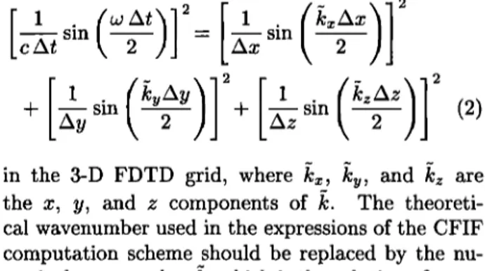
in the 3-D FDTD grid, where

•x, •v, and •z are

the x, y, and z components of k. The theoreti-

cal wavenumber used in the expressions of the CFIF

computation scheme should be replaced by the nu-

(4)

2192 O•UZ AND G•REL: IMPROVING ACCURACY OF PLANE WAVE EXCITATIONS

tion (2). By doing so, the theoretical and numerical

phase velocities are matched and the dispersion error

is significantly decreased.

In order to quantify the errors created in the plane wave generation process, the excitation and propa-

gation of waves in a homogeneous media are consid-

ered. A 3-D empty computational domain composed of 30 x 30 x 30 Yee cells and terminated by eight-cell- thick perfectly matched layers (PML) is set up for

this purpose. The PML walls are designed to have a

theoretical

normal

reflection

ratio R(0) of 10

-4 and

parabolic conductivity profile. The space sampling period is A -- 0.625 cm. The time step is selected at the Courant stability limit as At - 12.081 ps. Separate-field formulation is employed with a total- field region of 18 x 18 x 18 cells and a six-cell-thick scattered-field region. The incident plane wave val- ues are computed with the CFIF scheme. The plane wave is incident at 0 - 90 ø and •5 = 45 ø. The in- cident electric field is polarized in the z direction, and its amplitude is unity. The incident magnetic

field is polarized in the direction of & -•. The time

dependence of the incident plane wave is given by

e(t) = w(t) sin (2•rf0t),

where f0 = 1 GHz and w(t) is either the unit step

function or a Hanning window defined as

0, t <_ 0,

-

0.5- 0.5 cos

0 < <

1, otherwise.

(4)

Note that w(t) becomes a unit step function when

L - 0. For L > 0, the Hanning windows help reduce the FDTD errors due to the high-frequency compo-

nents of the excitation signal by smoothing the time

dependence of the incident plane wave [Giirel and O•uz, 1997].

Ideally, the fields in the total-field region of the FDTD grid should be exactly the same as the in- cident plane wave, and the field variables in the scattered-field region should be identically equal to zero. However, owing to the approximate nature of

the FDTD method, numerical field variables are ex-

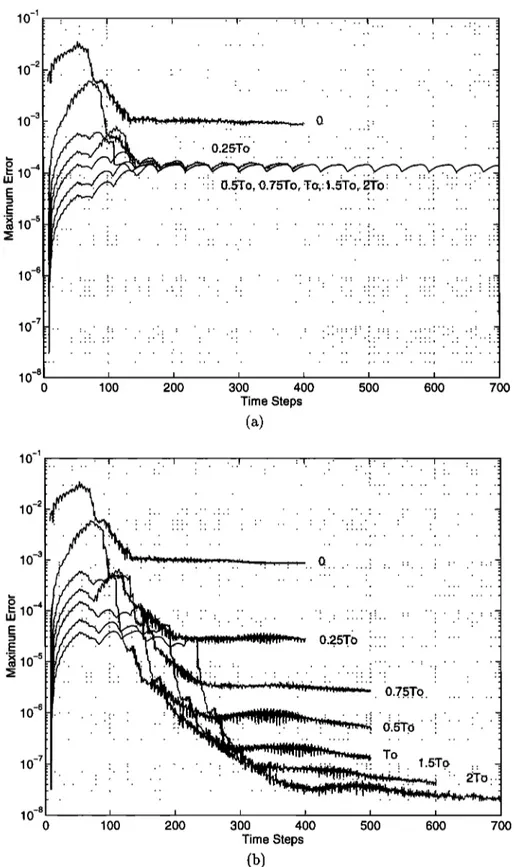
pected to deviate from their ideal counterparts. The deviation, that is, the error, can be computed at each time step, in every cell, and for any field component. Figures 2a and 2b show the maximum value of the error in the E• component over both the total-field and scattered-field domains at each time step. Fig-

ure 2a is obtained using the theoretical wavenumber

k, whereas

Figur_e

2b is obtained

using

the numeri-

cal wavenumber k. These error results are obtained

by using Hanning windows of lengths L = 0, 0.25T0,

0.5T0, 0.75T0, To, 1.5T0, and 2T0, where To = lifo

is the period of the sinusoidal time dependence of the incident plane wave. The input signal is multi- plied by a smoothing window at early times in or-

der to decrease the errors due to the abrupt change

at the onset of the input signal which has high-

frequency components [Giirel and Oyuz, 1997]. The

zero-length window corresponds to no smoothing at

the input. Figures 2a and 2b show that the high-

frequency errors are dominant when no window is

used. Increasing the window length to L = 0.25To

improves the results. Figure 2a shows that no fur-

ther improvement is obtained as the window length is

further increased using the theoretical wavenumber.

This is due to the threshold of dispersion errors at

this level. On the other hand, Figure 2b shows that

threshold level due to the dispersion errors can be significantly reduced using the numerical wavenum-

ber so that the improvements on the maximum error

become visible as the window length is increased be-

yond L - 0.25T0. Note that the window length af-

fects the high-frequency errors but not the dispersion

errors, and these results testify to the importance of

using

the numerical

wavenumber

• in the CFIF com-

putation scheme.

The numerical dispersion parameters are employed

in a different way in the IFA computation scheme. The numerical phase velocities of the incident waves in both the 1-D and the 3-D grids are calculated us-

ing equations (1) and (2). Then, the ratio of these

velocities is used to modify the permittivity and the

permeability values used in the FDTD equations of the 1-D source grid as

At

1/2

_ Hn-1/2

H'n+m+l/2

InC•

- inc,

mq-1/2

4'

'Op(O

--

O,

q5

--

0)]

X (E?nc,

m - E?nc,

m+l) ,

(5)

At n+l n

Einc,

m -- Einc,

m +

Op(O

--

O,

(/5

--

O)

A •5

0 ¸p(O,

qS)

(H,n+l/2 _ Hn+

•/2

X \ inc,

m--i/2 inc,

re+l/2)

'

(6)

(5)

O(•UZ AND GOREL: IMPROVING ACCURACY OF PLANE WAVE EXCITATIONS 2193 10 -2 0 -5 ' : 10 -6 .

10-7

:i ! i . ' :

10 -8 0 100 200 300 400 500 600 700 Time Steps (a) 10 -3

0-4

0-5 0.'25To ... .... ::: .:... ... ... : :.0:7.5.To..: ;.:: :. .:: .... 10 -6 ::::::::::::::::::::::::::: ß ... !!!:.':.!:.!.!!!!' !! !!'!!:.!'!i: :. ':::: ::::::::::::::::::::: ... ... : ... .. ... : ...

10_

7 ...

. ....

TO -1,5..'17:0.

: 10 -8 0 100 200 300 400 500 600 700 Time Steps

Figure 2. Plots of maximum error on Ez obtained by using different lengths of smoothing windows and (a) theoretical and (b) numerical wavenumbers.

(6)

2194 O(•UZ AND G•REL: IMPROVING ACCURACY OF PLANE WAVE EXCITATIONS numerical phase velocities in the two grids, which

is crucial for an accurate excitation of the 3-D grid

by the 1-D IFA [Taftore, 1995]. Results obtained

using the IFA excitation scheme with the numerical

wavenumber and employing various orders of inter-

polation are presented in the next section.

4. Incident Field Array (IFA) With

Higher-Order Interpolation

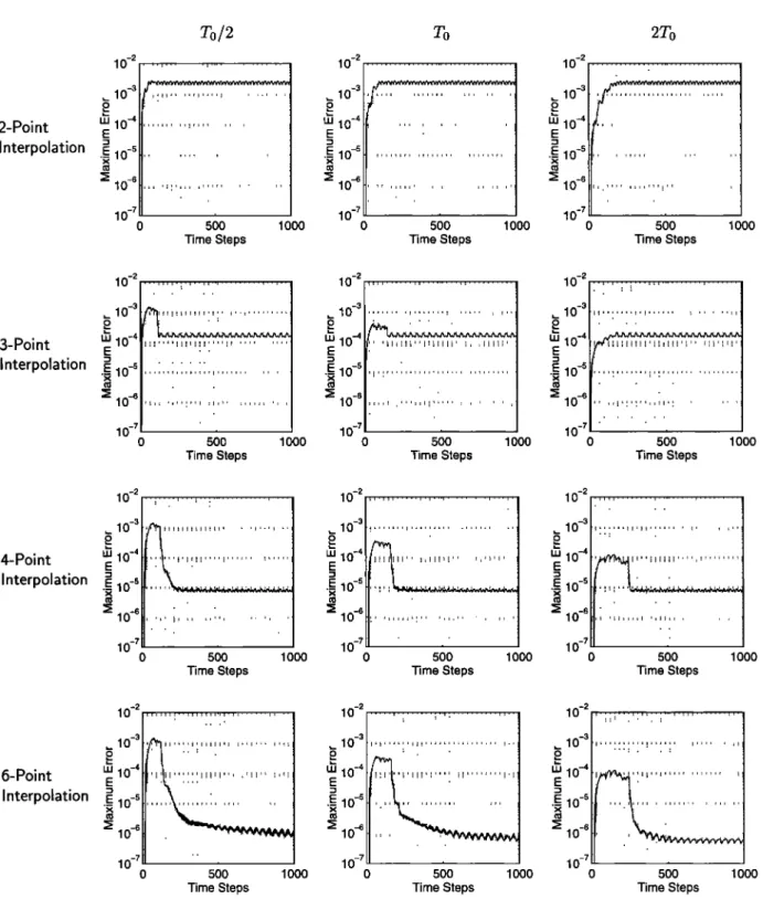
The top row of error plots shown in Figure 3 is ob- tained by using the numerical wavenumber and em-

ploying linear interpolation as originally suggested by

Taftore [1995]. By comparing these relatively high

error levels with those of Figure 2b for the same win- dow lengths, one can easily conclude that although the IFA computation scheme is quite efficient, it is not as accurate as CFIF. However, it is possible to in-

crease the accuracy of the IFA scheme by increasing

the interpolation order in the computations. When the interpolation order is increased, the incident-field

values are related to more points in the 1-D source

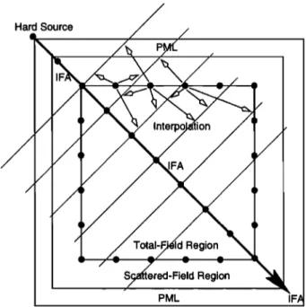
grid. The geometry of the IFA scheme using cubic

(4-point) interpolation is shown in Figure 4. As the

IFA computation of an incident-field value uses more 1-D vector elements, the quality of the output also in-

creases. In a linear (two-point) interpolation scheme,

a straight line is assumed to pass through the two points. This is a rough estimate for curved func- tions such as sinusoidals. Higher-order polynomials,

such as parabolas or cubic curves, are more suitable

to model the variation of the incident wave. There-

fore increasing the interpolation order decreases the

error in the IFA computations. This improvement is depicted in Figure 3, where the results obtained by using Hanning windows of lengths 0.5 To, To, and 2 To are shown for linear, quadratic, cubic, and fifth-

order polynomial interpolation schemes. With the

fifth-order interpolation, it is possible to achieve re- sults close to the CFIF results. Using a half-period- long Hanning window and a fifth-order interpolation scheme, the resulting error level is very close to that of the CFIF result, for which the same length of smoothing window is used. Moreover, the IFA tech- nique is still efficient with respect to the CFIF tech-

nique, as will be discussed in the next section.

The results of this section imply that together with

the aliasing errors due to high-frequency components

[Giirel and O•uz, 1997] and the numerical dispersion [Taftore, 1995], the interpolation order has a signifi-

cant role in determining the error level in the plane

wave excitations. As long as the smoothing windows

suppress the high-frequency components sufficiently

and the phase velocities are matched, the maximum error level can be controlled by varying the interpo-

lation order.

The usefulness of the error-reducing techniques

presented in this section are demonstrated using plane

wave excitations with sinusoidal time dependence. However, the applicability of these higher-order in-

terpolation techniques is not limited to the sinusoidal

time dependence; they are valid for any arbitrary

time dependence of the plane waves.

5. Efficiency of the IFA

A simple experiment is set up to test the efficiency of the IFA technique with higher-order interpolation. One million sinusoidal functions are computed with closed-form expressions, and the computation time is compared with the time spent to perform one mil- lion linear, cubic, and fifth-order polynomial inter- polations. The experiment is carried out on a Sun- SPARC10 workstation. The computation times are given in Table 1.

Clearly, even the fifth-order interpolation is more

efficient than computing a simple sinusoidal function.

If a smoothing window is used, which means that a

second sinusoidal term has to be computed, or if an

incident wave with a more complicated expression is propagated, the computation time for the CFIF scheme increases; however, the computation times

remain the same for the IFA scheme regardless of

the input expression.

By examining Table I and Figure 3 together, one can see the trade-off between the accuracy of the re- sults and the efficiency with which they are com- puted. It is important to know that the IFA scheme

is more efficient than the CFIF scheme even when

fifth-order interpolation is used to obtain highly ac-

curate results.

The computational complexity of an n-dimensional FDTD problem with a total of N grid points is

O(Nn+l/n), where

the extra factor of O(N l/n) is

due to the number of time steps [Chew, 1990].

Therefore, for a 3-D FDTD problem, the compu-

tational

complexity

is O(N 4/3) since

the number

of

time steps

is proportional

to N 1/3. The interpola-

tion operations are carried out on a closed surface,

namely, on the total-field/scattered-field boundary.

On this connecting boundary, the interpolation oper-

(7)

O•UZ AND G•REL: IMPROVING ACCURACY OF PLANE WAVE EXCITATIONS 2195 z0/ 10 -2 :::::::::::.::::.:'..• • • • ...

10 -3 ...,.,,

,•,•

o :::::::"::::::.:: ... 2-Point '" lO-4 ß .

[nterpolation

.• lO-5

x ... :: ... :.::: ... :: .... (1• ';'...::::.::::.;

• 10-6 ...

... ... 10 -7 ... 0 500 1000 Time Steps To 10 -2 i•:•!!•.:•!.::,:: ::::::: ::::: !!!!!!:!!::!!!:!'!!':: ... .":': 0 LU 10 -4

:3 0

-5 ... :::.

..

.x

E

- 1

_O•

...

_:::: _:' _:::.' _:.:: _'..

• 10-6 ...

.. ... 10_7 ... 0 500 1000 Time Steps 10 -2 !::!!!!:!!!:!!!!!! ...

$ 10-3

,•.,.•,•

.

....

•_ . . LU 10 -4

ß

x

E-

10 -5 ...

(1• ;';;'::::;;;;::;: .

:• 10-6 ...

... ... 10_7 ... 0 500 1000 Time Steps 3-Point Interpolation 10 -2 p

I• 10 -4 ,,,,,:,,,..,,,,i•:•, ... •.•.i•

ß

• 10

-s ....

t• :!!::!!!!!!!!::!:!! ... . ....

• 10-6 ...

... .. ... ... ... 10 -7 0 500 1000 Time Steps 10 -2 :::::":::::: ::x: ... 10-3 ß ... ß ... 10 -4

0_

5 ... ".

.•1

::::::::::::::::::::::::::::: ::.

10-6

...

... .. :::.: .:::...:.::. .' 10_7 ... 0 500 1000 Time Steps 10 -2 10 -3 o LU 10 -4 E

.x

E-

10 -5

.. ß., ...

:• 10-6

...

... ... 10 -7 ... 0 500 1000 Time Steps 10 -2 10 -3 o 4-Point LU _E10-4

Interpolation

.•_

x

10-5

• 10-6 ...

... ;:.;.::..::::::..: ... ... 10 -7 ... 0 580 1000 Time Steps 10 -2 10 -3 o LU 10 -4 E

ß

• 10

-5

• 10-6 ...

... ... ... 10 -7 ... 0 580 1000 Time Steps 10 -2 .... 10-3 • !:!!!!:!!!!!::i::! ... . ... I• 10 -4

"' 0-

5 ß

(•

1 : ::

::

::::

::

::::::::

:::::

::

• 10-6 ...

... ... ... 10_7 ... 0 500 1000 Time Steps 10 -2 ... ... ,_ 10 -3 ::::::::::::::::::::::::::::: ::::::::::::,::,: ::: :: :: 6-Point '" lO-" • • • .: ... • !: • • •:• ..:::::: ::::::• E

[nterpolation

.• lO-5

! ! .-' .' ' '.- i ! i'..' ! ! ' ! -• ! !

"

•; 10-6

... ... ... .... ... 10_7 ... 0 500 1000 Time Steps LU 10 -4 E

"' 0-

5 ß

• 1

• 10-6

10 -2 :.::::::.:.:::::.:: ... ;:: ... ... ... ... ... 10 -7 ... 0 500 1000 Time Steps 10 -2 ,_ 10 -3 o LU 10 -4 E

"' 0-

5 ß

• 1

• 10-6

10 -7 0 ß ... ... ... 5OO Time Steps 1000

Figure 3. Plots of maximum error levels obtained by using various window lengths and interpolation orders.

(8)

2196 O(•UZ AND G•REL' IMPROVING ACCURACY OF PLANE WAVE EXCITATIONS

Hard Source

Id Region

Region

PML IF,•

Figure 4. The IFA excitation scheme with in-

creased interpolation order. Incident-field values in the 3-D computational domain are interpolated from the closest four elements on the 1-D source grid. time steps. Hence the interpolation operations have a total computational complexity of O(N), which is lower than the complexity of the 3-D FDTD algo- rithm. Therefore, no matter how high the order is,

the interpolation scheme does not add any significant

computational cost to the FDTD algorithm.

6. Scattering Results With

Higher-Order Interpolation

The effects of using higher interpolation orders can

be demonstrated

by a scattering

prbi•em.

A square

metal plate of size 20 x I x 20 Yee cells is modeled

for this purpose. The plate lies on the x-z plane, in

the middle of a computational domain consisting of

Table 1. Computation Times for the CFIF Scheme and the IFA Scheme Using Various Orders of Interpolation Scheme Time, s CFIF 5.46 IFA Linear 0.57 Cubic 2.11 Fifth-order 3.99

40 x 20 x 40 cells, which is divided into a total-field

region of 28 x 8 x 28 Yee cells and a six-cell-thick scattered-field region. The incident plane wave is

identical to the one in section 3.

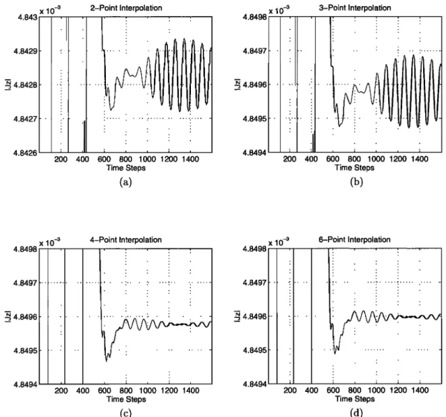
The results presented in Figure 5 show the ampli- tude of the z component of the induced surface cur-

rent Jz at an arbitrary point on the plate. The am-

plitudes of Jz signals are computed at every time step

with a two-point amplitude-detection scheme, as out- lined in the appendix. The amplitude plots of Fig- ures 5a-5d are obtained by using linear, quadratic,

cubic, and fifth-order interpolation schemes, respec-

tively. A Hanning window of length 0.5 To is used in all simulations. Figure 5 shows the improvement in

the convergence error of the [Jz[ variable as the in-

terpolation order is increased. The results obtained with two-point interpolation in Figure 5a converge to a completely different value than the others. The amplitudes of the steady state oscillations in Fig-

ure 5b are decreased to a much lower level in Fig-

ure 5c by changing the interpolation from quadratic to cubic. Increasing the interpolation order to 5 in Figure 5d makes no significant improvement on the results obtained by cubic interpolation in Figure 5c. However, there is a slight difference in the ampli- tude levels that the two signals converge to. These results demonstrate various degrees of improvement

obtained by using progressively higher orders of in-

terpolation. Compared with the steady state value depicted in Figure 5d, the errors in Figures 5a-5c

are 0.14%, 0.0021%, and 0.00062%, respectively, for

the induced surface current on the patch. Similarly, the RCS values computed from the currents of Fig- ure 5a are 0.13% in error compared with the that of the Figure 5d.

7. Conclusions

In this paper, we have demonstrated that match- ing the phase velocity of the incident plane wave to the numerical phase velocity imposed by the numer-

ical dispersion of the 3-D FDTD grid is crucial for

obtaining accurate plane wave excitation. This ob-

servation holds for both the CFIF and the IFA exci-

tation schemes in the separate-field formulation. In

general, the IFA scheme is more efficient than, but

not as accurate as, the CFIF scheme. We have shown

that it is possible to increase the accuracy of the

IFA scheme by using higher-order interpolation tech-

niques in the process of transferring the incident-field

(9)

O(•UZ AND G•REL' IMPROVING ACCURACY OF PLANE WAVE EXCITATIONS 2197 X 10 -3 4.843 4.8429 N 4.8428 4.8427 4.8426 200 400 2-Point Interpolation 600 800 1000 1200 1400 Time Steps 4.8498 4.8497 4.8496 4.8495 4.8494 x 10 -3 3-Point Interpolation 200 400 600 800 1000 1200 1400 Time Steps x10 -s 4.8498

_

N 4.8496

4.8497

4.8495 4.8494 200 400 4-Point Interpolation ß . .

o'oo

ioo

Time Steps (c) X 10 -3 4.8498 4.8497 4.8496 4.8495 4.8494 200 400 6-Point Interpolation

o'oo

;oo

Time Steps

Figure 5. Amplitude plots for Jz at a single point on the surface of a metal plate us-

ing a Hanning window of length L - To/2. The interpolation schemes are (a) linear, (b) quadratic, (c)cubic, and (d)fifth-order.

These higher-order interpolation techniques can be used for the excitation of plane waves with arbitrary time dependence.

Appendix: Two-Point Amplitude and

Phase Detection

Figure 5 presents amplitude plots of a current com- ponent as the result of a scattering problem. The

amplitudes and phases of the sinusoidal steady state

signals are computed with a simple but accurate

method. Assuming a discrete sequence obtained by

sampling a pure sinusoidal signal, the amplitude and

phase values can be extracted from two consecutive

samples. The signal values at these time steps can

be written as

Asin (a•tl -]- •b) -- ½1, (A1) Asin(wt2-Fc•) - c2, (A2)

where the time instants tx and t• are related to each other by

t2 -- tl -F At. (A3)

(10)

2198 O(•UZ AND G•REL' IMPROVING ACCURACY OF PLANE WAVE EXCITATIONS

with two unknowns. The unknown parameters are A and •5, the amplitude and phase of the signal. Solv-

ing equations (A1) and (A2) for these two unknowns

yields

•5 arctan

-

(cot

coat

c2

cscwAt - t•,

)

(A4)

c1

A - csc

wAtV/(c•

sin

war)2+

(Cl

cos

war

- c2)2.

(A5)

Note that most of the trigonometric operations in the above are independent of t•, t2, c•, and c2. Thus they can be computed only once and used several

times. Then, equations (A4) and (A5) require the

computation of one inverse tangent and one square

root operators. Therefore equations (A4) and (A5)

can be efficiently used at any two consecutive time instants, perhaps at every FDTD time step. By do- ing so, one can easily and efficiently keep track of

the convergence of the signals to their steady state

values, without having to wait several periods of the signal after the convergence.

Equations (A4)and (A5)are derived assuming

perfect sinusoidals. Thus any perturbations on the

finite difference data distort the phase and ampli- tude computations. However, this distortion is in

the same order as the amplitude of the error on the input signal. Therefore the two-point algorithm does

not decrease the accuracy set by the FDTD method.

Acknowledgments. The authors would like to

acknowledge an anonymous reviewer for his/her

meticulous review, which significantly improved the manuscript, and Bijan Houshmand for his useful sug- gestions and careful review of the manuscript.

References

B•renger, J.-P., A perfectly matched layer for the absorption of electromagnetic waves, J. Comput.

Phys., 114, 185-200, 1994.

B•renger, J.-P., Perfectly matched layer for the FDTD solution of wave-structure interaction prob- lems, IEEE Trans. Antennas Propag., dd(1), 110-

117, 1996a.

B•renger, J.-P., Three-dimensional perfectly matched

layer for the absorption of electromagnetic waves,

J. Cornput. Phys., 127, 363-379, 1996b.

Chew, W. C., Waves and Fields in Inhomogeneous Media, Van Nostrand Reinhold, New York, 1990.

DePourcq, M., Field and power-density calculations in closed microwave systems by three-dimensional

finite differences, IEE Proc. Part H, Microwaves

Antennas Propag., 132(6), 360-368, 1985.

Deveze, T., L. Beaulie, and W. Tabbara, A fourth order scheme for the FDTD algorithm applied to Maxwell equations, IEEE Antennas and Propag. Soc. Int. Symp., 1, 346-349, 1992.

Fang, J., Time domain finite difference computation for Maxwell's equations, Ph.D. thesis, Univ. of Calif. at Berkeley, 1989.

Gfirel, L., and U. O•uz, Signal-engineering

techniques to reduce the sinusoidal steady- state error in the FDTD method, Res. Rep.

BILUN/EEE/LG-9701, Bilkent Univ., Ankara,

Turkey, 1997.

Harrington, R. F., Field Computation by Moment Methods, Krieger, Melbourne, Fla., 1982.

Kunz, K. S., and R. J. Luebbers, The Finite Differ- ence Time Domain Method for Electromagnetics, CRC Press, Boca Raton, Fla., 1993.

Lindman, E. L., "Free-space" boundary conditions

for the time dependent wave equation, J. Comput.

Phys., 18, 66-78, 1975.

Manry, C. W., S. L. Broschat, and J. B. Schneider, Higher-order FDTD methods for large problems,

Appl. Cornput. Electrornagn. $oc. J., 10(2), 17-29,

1995.

Merewether, D. E., Transient currents on a body of revolution by an electromagnetic pulse, IEEE

Trans. Electrornagn. Cornpat., 13(2), 41-44, 1971.

Merewether, D. E., R. Fisher, and F. W. Smith, On implementing a numeric Huygen's source scheme in a finite difference program to illuminate scat-

tering bodies, IEEE Trans. Nuclear Sci., 27(6),

1829-1833, 1980.

Miller, E. K., L. Medgyesi-Mitschang, and E. H.

Newman (Eds.), Computational Electromagnetics,

Inst. of Electr. and Electron. Eng., New York,

1992.

Mur, G., Absorbing boundary conditions for

the finite-difference approximation of the time- domain electromagnetic-field equations, IEEE

Trans. Electrornagn. Cornpat., EMC-23(4), 377-

382, 1981.

Omick, S. R., and S. P. Castillo, A new finite-

difference time-domain algorithm for the accurate

modeling of wide-band electromagnetic phenom- ena, IEEE Trans. Electromagn. Cornpat., EMC-

35(2), 215-222, 1993.

Shlager, K. L., and J. B. Schneider, A selective sur-

vey of the finite-difference time-domain literature,

(11)

O•UZ AND G•REL: IMPROVING ACCURACY OF PLANE WAVE EXCITATIONS 2199

Tafiove, A., Application of the finite-difference

time-domain method to sinusoidal steady-state electromagnetic-penetration problems, IEEE

Trans. Electromagn. Cornpat., EMC-22(2), 191-

202, 1980.

Tafiove, A., Review of the formulation and applica-

tions of the finite-difference time-domain method

for numerical modeling of electromagnetic wave in-

teractions with arbitrary structures, Wave Mo-

tion, •0(6), 547-582, 1988.

Tafiove, A., Computational Electrodynamics: The Finite-Difference Time-Domain Method, Artech

House, Norwood, Mass., 1995.

Tafiove, A., and M. E. Brodwin, Numerical solution of steady-state electromagnetic scattering prob- lems using the time-dependent Maxwell's equa-

tions, IEEE Trans. Microwave Theory Tech.,

MTT-23(8), 623-630, 1975.

Tafiove, A., and K. Umashankar, Radar cross sec- tion of general three-dimensional scatterers, IEEE

Trans. Electromagn. Cornpat., EMC-25(4), 433-

440, 1983.

Tafiove, A., and K. R. Umashankar, Review of FD- TD numerical modeling of electromagnetic wave scattering and radar cross section, Proc. IEEE,

77(5), 682-699, 1989.

Tafiove, A., K. R. Umashankar, and T. G. Jurgens,

Validation of FD-TD modeling of the radar cross

section of three-dimensional structures spanning

up to nine wavelengths, IEEE Trans. Antennas

Propag., AP-33(6), 662-666, 1985.

Umashankar, K. R., and A. Tafiove, A novel

method to analyze electromagnetic

scattering

of

complex objects, IEEE Trans. Electromagn. Corn-

pat., EMC-24(4), 397-405, 1982.

Yee, K. S., Numerical

solution

of initial boundary

value problems involving Maxwell's equations in

isotropic

media, IEEE Trans. Antennas

Propag.,

AP-14(4), 302-307, 1966.

L. Gfirel, Department of Electrical and Electronics

Engineering,

Bilkent University,

TR-06533,

Bilkent,

Ankara,

Turkey.

(e-mail:

lgurel¸bilkent. edu.tr)

U. O•uz, Department of Electrical and Electronics

Engineering,

Bilkent University,

TR-06533, Bilkent,

Ankara, Turkey.