Pairing in charged-neutral fermion mixtures under an artificial magnetic field

PAIRING IN CHARGED-NEUTRAL

FERMION MIXTURES UNDER AN

ARTIFICIAL MAGNETIC FIELD

a thesis

submitted to the department of physics

and the graduate school of engineering and science

of bilkent university

in partial fulfillment of the requirements

for the degree of

master of science

By

Fatma Nur ¨

Unal

August, 2012

I certify that I have read this thesis and that in my opinion it is fully adequate, in scope and in quality, as a thesis for the degree of Master of Science.

Assoc. Prof. Dr. Mehmet ¨Ozg¨ur Oktel (Advisor)

I certify that I have read this thesis and that in my opinion it is fully adequate, in scope and in quality, as a thesis for the degree of Master of Science.

Prof. Dr. O˘guz G¨ulseren

I certify that I have read this thesis and that in my opinion it is fully adequate, in scope and in quality, as a thesis for the degree of Master of Science.

Prof. Dr. Bayram Tekin

Approved for the Graduate School of Engineering and Science:

Prof. Dr. Levent Onural Director of the Graduate School

ABSTRACT

PAIRING IN CHARGED-NEUTRAL FERMION

MIXTURES UNDER AN ARTIFICIAL MAGNETIC

FIELD

M.S. in Physics

Supervisor: Assoc. Prof. Dr. Mehmet ¨Ozg¨ur Oktel August, 2012

Bose-Einstein condensations (BEC), pairing behaviour, vortex formations in su-perconductivity and superfluidity are just a few examples of fascinating features of ultracold gases. In this thesis, we study charged-neutral cold atom mixtures which are obtained by placing a neutral mixture under an artificial magnetic field coupling only one of the components. We begin with two distinguishable (charged-neutral) particles on a ring trap. Charged particle gains angular mo-mentum due to a magnetic field along the axis of the ring and we see that there is a big angular momentum transfer to neutral particle in orders of ¯h. This work

is set forth to guide us in the many body problem of vortex transformation in charged-neutral superfluid mixtures. In the main part of the thesis, we examine charged-neutral fermion mixtures. Thanks to artificial magnetic fields, Cooper pairs whose only one component coupling to magnetic field can be created now. We calculate the gap equation for this system and solve for the critical temper-ature. We show that critical temperature decreases for the increasing magnetic field.

Keywords: Pairing, superconductivity, charged-neutral mixture, artificial

mag-netic field, pairing susceptibility, gap equation. iii

¨

OZET

YAPAY MANYET˙IK ALAN ALTINDA

Y ¨

UKL ¨

U-Y ¨

UKS ¨

_{UZ KARIS.IMLARDA ES.LENME}

Fatma Nur ¨Unal Fizik, Y¨uksek Lisans

Tez Y¨_{oneticisi: Doc.. Dr. Mehmet ¨}Ozg¨ur Oktel A˘gustos, 2012

As.ırı-so˘guk gazların etkileyici pek c.ok ¨ozelli˘gine Bose-Einstein yo˘gunlas.ması (BEY), es.lenme davranıs.ı, s¨uperiletken ve s¨uperakıs.kanlardaki girdap olus.umu ¨

ornek verilebilir. Biz bu tezde n¨_{otr bir karıs.ımı biles.enlerinden yalnızca} biriyle c.iftlenen yapay bir manyetik alanın etkisinde bırakarak elde edilebilen y¨ukl¨u-n¨_{otr karıs.ımları inceledik.} C_{. alıs.mamıza halka bir kapan ¨}uzerindeki iki tane ayırt edilebilir (y¨ukl¨u-n¨_{otr) parc.acıkla bas.ladık.} Y¨ukl¨_{u parc.acık} halkanın ekseni y¨on¨undeki manyetik alan y¨uz¨_{unden ac.ısal momentum kazanırken,} n¨_{otr parc.acı˘ga da y¨uksek miktarlarda ac.ısal momentum transferi oldu˘gunu} g¨_{ozlemledik. Bu hesaplamanın temel amacı c.ok parc.acık problemimizde,} y¨ukl¨u-n¨otr s¨_{uperakıs.kan karıs.ımlardaki girdap transferi, bize yol g¨ostermesidir. Tezin} esas b¨ol¨um¨unde, y¨ukl¨u-n¨_{otr fermiyon karıs.ımları inceledik. Yapay manyetik} alan-lar sayesinde, sadece tek bir biles.eni manyetik alanla c.iftlenen Cooper c.iftleri artık yaratılabiliyor. Bu sistem ic.in aralık denklemini yazıp, kritik sıcaklık de˘gerini hesapladık. Kritik sıcaklı˘_{gın artan manyetik alana kars.ı d¨us.t¨u˘g¨un¨u g¨osterdik.}

Anahtar s¨ozc¨ukler : S¨uperiletkenlik, y¨ukl¨u-n¨_{otr karıs.ımlar, yapay manyetik alan,} es.lenme duyarlılı˘gı, aralık denklemi.

Acknowledgement

I would be sincerely happy to present my deepest gratitude to my supervisor Assoc. Prof. Dr. Mehmet ¨Ozg¨ur Oktel. My respect to him, his kindness and his knowledge is endless. During this one year we have studied together, he started teaching me cold atoms. But, besides these special lectures, I have learned a lot directly from him when we were trying to cope with an integral or when he was commenting on a paper.

I would like to also thank Prof. Dr. O˘guz G¨ulseren and Prof. Dr. Bayram Tekin for their time to read and review this thesis. Asst. Prof. Balazs Het´enyi deserves special thanks. Even if I could not have a chance to take a course of him, he has been always generous and willing to explain me something that I struggled in physics and it was my pleasure to talk quantum mechanics with him.

I am grateful for having a groupmate like Semih Kaya. We have spent lots of time by discussing our researchs and I am sure we will. Ertu˘grul Karademir has been always ready for brain-storming on physics, technology and science. I want to thank him for being really helpful and kind to me. I should also add my thanks to my colleagues and friends Ege ¨Ozg¨_{un, Ays.e Yes.il, Togay Amirahmedov} and thanks to G¨ozde G¨_{uc.l¨uler for being an excellent housemate. It would be not} enough to say how thankful I am to Sadi Ayhan for his help and moral support about this thesis, living in Ankara and in general about life.

I am also happy to have a chance at last to thank T ¨UB˙ITAK - B˙IDEB for supporting me financially throughout my undergraduate and M.S. study.

Finally, my deepest thanks and love are to my mother Sermin ¨Unal, my father Bilal ¨Unal, my sisters M. Hande and Z. Sena ¨Unal. They have not given up even one second to encourage me through my life and always been ready to help me when I failed in anything. I would not have been here if I did not always have them with me.

Contents

1 Introduction 1

1.1 Ultracold Atoms . . . 1

1.2 Artificial Magnetic Fields . . . 2

1.3 Charged-Neutral Mixtures . . . 3

2 Two-Particle Problem 5 2.1 Analytic Calculation . . . 5

2.1.1 Hamiltonian . . . 5

2.1.2 Angular momentum transfer . . . 8

3 Fermions: Superconductivity 11 3.1 Superconductivity . . . 11 3.1.1 Type-I superconductors . . . 11 3.1.2 Type-II superconductors . . . 12 3.2 BCS Theory . . . 12 3.2.1 Hamiltonian . . . 13 vi

CONTENTS vii

3.2.2 Gap equation . . . 15

3.2.3 Zero-temperature gap & Critical temperature . . . 16

3.2.4 Pairing susceptibility . . . 18 4 Fermion Problem 21 4.1 Approximation Schemes . . . 21 4.1.1 Particle densities . . . 21 4.1.2 Hamiltonian . . . 25 4.2 Pairing susceptibility . . . 28 4.3 Gap equation . . . 29

List of Figures

2.1 Energy levels vs. interaction potential, for L = 0 and β = 0.2 . . . 7 2.2 Energy levels vs. flux, for ˜U = 0.1 . . . . 8 2.3 Angular momentum of the neutral particle vs. interaction

poten-tial, for L = 0 and β = 0.2 . . . . 9

3.1 Critical magnetic field as a function of temperature for type II superconductors. . . 12 3.2 Temperature dependence of the energy gap. . . 18

4.1 Critical temperature vs. magnetic field. Landau levels can be seen at γ = _2n+11 . . . . 32

Chapter 1

Introduction

1.1

Ultracold Atoms

Observing quantum mechanics directly in laboratories is not that easy since most of the time it deals with systems in atomic levels. However, cooling the atoms down to near absolute zero brings the fascinating macroscopic quantum effects [1–5] to light by revealing Bose-Einstein Condensation (BEC). Particles in a BEC occupy the lowest state in large numbers and move much more slower due to the low temperatures [6, 7]. They start coherently acting more like waves which is evidently resulting in a convenient choice to study quantum mechanical effects in macroscopic scales. In other words, in this ultracold systems, there is no temperature fluctuations and no impurities, hence, high degree of control on this systems makes them proper quantum laboratory to examine few or many body phenomena.

A condensate state of atomic gases is first predicted in 1925 by Einstein and observed in 1995 at NIST-JILA laboratory [8]. This new state stands out by combining interests of several fields like atomic, condense matter, statistical and nuclear physics. Besides, achievements in ultracold atoms did not remain limited with boson, instead, more exotic phenomena have come out such as: fermion

CHAPTER 1. INTRODUCTION 2

superfluidity [1], BEC of photons [9], Feshbach resonance [6] and even some ap-plications in nuclear physics and astrophysics. As a recent success, we are served up with artificial magnetic fields.

1.2

Artificial Magnetic Fields

Ultracold atoms provide the abundant environment to observe pure many-body phenomena. Nevertheless, neutrality of the condensates constrains the search of effects originating from magnetic field, such as fractional quantum Hall effect [10] This obstacle is tried to be overcome first by rotating the condensate and using the resemblance between Lorentz and Coriolis force [11, 12]. However, because of the physical limitation of rotating the systems, high magnetic fields are disallowed for this method. Spielman et al. developed a method to optically induce an effective magnetic field [13] and immediately drew attention by enabling unlimited strength of magnetic fields.

In quantum mechanics, potentials are more important rather than fields like in classical mechanics. Vector potential is entering the Hamiltonian in the form of H = _2m1 (¯h_i∇ − q ⃗⃗ A)2, so, the crucial part to have the effect of a magnetic field is q ⃗A together. Spielman et al. achieve this by using a spatially dependent

Hamiltonian which results in an artificial magnetic field due to ⃗B = ⃗∇× ⃗A. They

first dress the internal (spin) states by two counter propagating laser beams with different momentum, then apply a spatially varying Zeeman shift. Observation of vortices in the condensate proves the presence of an effective magnetic field. Therefore, they obtain an optically synthesized magnetic field as a result of the position dependent light-matter coupling and spare us from the trouble of rotating the system. This procedure is delicately dependent on the internal degrees of freedom, so simply, it is almost impossible to create one that is coupling to both components of a neutral mixture.

CHAPTER 1. INTRODUCTION 3

1.3

Charged-Neutral Mixtures

In this thesis, we examine charged-neutral mixtures which is becoming more and more important after the discovery of synthetic magnetic fields. Under an artifi-cial magnetic field coupling to only one of the components of a neutral mixture (of particles, superfluids, condensates, etc...), we effectively attain a charged-neutral mixture. They allow the study of more exotic regimes of particle interactions than the neutral cold atom systems offer.

Initially, in the 2nd chapter of this thesis, we consider a charged-neutral two-particle mixture. We put them on a ring trap and introduce a short-range delta function interaction between them. Charged particle ( or superfluid in many body case to be mentioned at the end of the chapter ) gains angular momentum by coupling to magnetic field and drags the neutral one due to the interaction. To calculate this angular momentum transfer to the neutral particle, we first set the Hamiltonian and solve for the wave function by applying standard boundary conditions. In addition, we discuss the application of the results of the two-particle problem to many body case.

Secondly, we treat charged-neutral fermion mixtures, this time by examining the pairing behaviour of fermions in the case of mixtures. For this reason, we first cover the microscopic theory of superconductivity in chapter 3 with a brief sum-mary of type-II superconductors where high field superconductivity (achievable by artificial magnetic fields) is expected to important. And then in chapter 4, we define our fermion problem as↓ spin particles coupling to the magnetic field while

↑ spin particles not. At the beginning, to balance the densities of the ↑ and ↓ spin

particles, which are going to form Cooper pairs, we study chemical potentials of them. Then by defining the Hamiltonian, we start calculating the gap equation for this system. We are particularly interested in critical temperature Tc, hence,

we use the pairing susceptibility method explained in the section 3.2.4 to come up directly with the gap equation at Tc. We first start solving it analytically as much

as possible and complement with a numerical code to achieve the dependency of

CHAPTER 1. INTRODUCTION 4

Finally in chapter 5, we summarize our results of the two-particle problem and its applications to further many-body problem. Then, we present our fermion problem, the procedure we have followed to obtain and solve the gap equation and our results. We conclude with a brief description of our future plans.

Chapter 2

Two-Particle Problem

We study two neutral particles on a ring trap under an artificial magnetic field along the axis of the ring which is coupling only one of the particles and eventually resulting in a charged-neutral mixture. The charged particle is expected to gain angular momentum due to the magnetic field. The question is when we put a short-range delta function interaction between them whether the charged particle drags the neutral one and if so in which amounts. Throughout this chapter, we calculate the amount of this angular momentum transfer.

2.1

Analytic Calculation

2.1.1

Hamiltonian

We first write down the Hamiltonian describing the system with same mass for both particles and ϕ1, ϕ2 as angles of respective particles on a (−π, π) symmetric

ring of radius R. [ 1 2mR2 (_¯h i ⃗ ∇1− q ⃗AR )2 − ¯h2 2mR2∇⃗2+ V (ϕ1, ϕ2) ] Ψ(ϕ1, ϕ2) = EΨ(ϕ1, ϕ2) (2.1)

First part is representing the standard Aharonov-Bohm effect [14] for a particle with charge q under a vector potential ⃗A. Radius of the ring is fixed so the

CHAPTER 2. TWO-PARTICLE PROBLEM 6

problem reduces to 1D. Interaction potential is initially defined as attractive,

V (ϕ1, ϕ2) = −uδ(θ) for relative angle θ = ϕ1 − ϕ2, but it could be smoothly

extended to cover repulsive interaction for negative values of u.

− ¯h2 2mR2 [ ∇2 1+∇22− 2i qR ⃗A ¯ h ⃗ ∇1− (_{qR ⃗A} ¯ h )2] Ψ(ϕ1, θ)− EΨ(ϕ1, θ) = uδ(θ)Ψ(ϕ1, θ) (2.2) We propose a solution in the form of Ψ(ϕ1, θ) = eiLϕ1f (θ). This wave function is

incorporating the total angular momentum conservation which is related with the first particle and an additional part arising from the coupling between particles. Initial state m1, m2 couples into m1+m2 = L and m1−m2. Such a form represents

the properties of the system besides simplifies the hamiltonian. For dimensionless energies ˜E = 2mR_¯h22E, ˜U = 2mR 2 ¯ h2 u and β = qR ⃗A ¯

h as flux quantum, the Hamiltonian

is eiLϕ1 [ 2∂ 2_f ∂θ2 + 2iL ∂f ∂θ − L 2_{f − 2iβ} ( ∂f ∂θ + iLf ) + ( ˜E− β2)f ] = 0 (2.3) 2 ¨f + 2i(L− β) ˙f + ( ˜E− (L − β)2)f = 0 (2.4) f (θ) = { f1(θ) = Aeλ+θ+ Beλ−θ ,−π < θ < 0 f2(θ) = Ceλ+θ+ Deλ−θ , 0 < θ < π (2.5) for λ_± = iβ−L₂ ±∆₂ where ∆ = √

(β− L)2− 2 ˜_{E. β and L always appear together}

in equations. Increasing L by 1 while decreasing β by 1 gives rise to the same state as before. This behaviour can be easily seen in Fig. 2.2, but before coming that we have to solve for constants by applying boundary conditions.

2.1.1.1 Boundary conditions

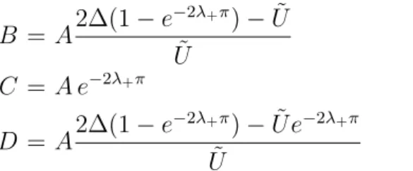
There are four boundary conditions: continuity of f (θ) at 0 and (−π, π), con-tinuity of derivative of f (θ) at (−π, π) and discontinuity of it at 0, which are respectively A + B = C + D (2.6) Ae−λ+π_{+ Be}−λ−π _{= Ce}λ+π_{+ De}λ−π _(2.7) A λ+e−λ+π+ B λ−e−λ−π = C λ+eλ+π + D λ−eλ−π (2.8) ∆(C− A) = − ˜ U 2(A + B) (2.9)

CHAPTER 2. TWO-PARTICLE PROBLEM 7

We solve for B, C and D in terms of A which is left to be determined by normal-ization. B = A2∆(1− e −2λ+π₎− ˜_U ˜ U (2.10) C = A e−2λ+π _(2.11) D = A2∆(1− e −2λ+π₎− ˜_{U e}−2λ+π ˜ U (2.12)

By solving boundary conditions, we obtain a relation between interaction poten-tial and energy of the system.

˜ U = 2∆ ( coth ∆π− cos (β− L)π sinh ∆π ) (2.13) It would be better to arrange Eq. (2.13) in reverse direction, but it has a nice and compact form in this way , so we leave it as it is. This equation tells us that ˜

E must be smaller than (β−L)₂ 2 (real ∆ solutions) for the system to be in bound state. And the system excites to an upper (n + 1)th _{state at ˜E =} (β−L)2

2 + (n+1)2

2

where we observe Feshbach resonance (dashed lines in Fig. 2.1) [15]. While the interaction is taken to the infinity, it suddenly swaps to minus infinity and the system jumps to the upper state.

−20 −15 −10 −5 0 5 10 15 20 −4 −2 0 2 4 6 8 Interaction Potential, ˜U E n e rg y L e v e ls , ˜ E Ground State 1st Excited 2nd Excited 3rd Excited

CHAPTER 2. TWO-PARTICLE PROBLEM 8

It should be remembered that we define interaction potential as attractive for positive ˜U. And as can be seen in Fig. 2.1, there is antisymmetry between attractive and repulsive potentials.

−1.50 −1 −0.5 0 0.5 1 1.5 0.5 1 1.5 2 2.5 3 3.5 4 Flux, β E n er g y L ev el s, ˜ E L_total=0 L total=1 L_total=2 L total=−1 L total=−2 L total=3 L total=−3

Figure 2.2: Energy levels vs. flux, for ˜U = 0.1 .

We mentioned (β − L) dependency before, Fig. 2.2 demonstrates this be-haviour. For example, if the system remains in ground state through flux quan-tum from −1.5 to 1.5, total angular momentum takes values of −1, 0 and 1 (this change in Ltot by integer numbers reminds vortices). We also examine the many

body correspondence of this system. We take a charged-neutral superfluid mix-ture under an artificial magnetic field and search for vortex transfer from charged superfluid to neutral one due to superfluid drag. This two-particle results and Fig. 2.2 lead us in many body problem to find the points where the vortex transfer might be present and to estimate the integration strength needed for it.

2.1.2

Angular momentum transfer

Due to the interaction of particles, the neutral one begins to gain angular mo-mentum, too. To achieve an equation for this angular momentum transfer, we

CHAPTER 2. TWO-PARTICLE PROBLEM 9

first normalize the wave function to find out last constant A, then calculate the average angular momentum of the neutral particle. < Ln> is calculated as below

in the bound state that is real ∆ solution.

< Ln>bound =− β 2 + π∆α sin βπ 2π((α− 1)e∆π− α cos βπ) + 2 ∆sinh ∆π (2.14) for α = 2∆_U˜.

Here, we again assume total angular momentum to be zero, therefore Eq. (2.14) itself is for the ground state, but it can be smoothly extended to cover other L values by replacing β with (β− L). For excited states, we calculate <Ln>scat by

taking ∆ imaginary, < Ln>scat=− β 2+ ∆π 2 sin βπ sin ∆π

π(1− cos βπ cos ∆π) − _∆2 sin ∆π sin πβ−∆₂ sin πβ+∆₂ (2.15) These results are represented in Fig. 2.3. As expected in ground state when

−20 −15 −10 −5 0 5 10 15 20 −2 −1.5 −1 −0.5 0 0.5 1 1.5 2 Interaction Potential, ˜U < L n > 1st Excited 2nd Excited 3rd Excited 4th Excited Ground State

Figure 2.3: Angular momentum of the neutral particle vs. interaction potential, for L = 0 and β = 0.2 .

CHAPTER 2. TWO-PARTICLE PROBLEM 10

the neutral particle possesses non-zero angular momentum which is remarkable because in bound state regime for small interactions angular momentum transfer is in order of ¯h.

All results are valid even in resonant interactions and crosschecked by per-turbative and numerical approaches of Semih Kaya [16]. They exhibit high con-sistency and guide us in the many body problem. However, for a many body or single particle problem usually perturbative approaches are used like we do with Gross-Pitaevskii [6] and Bogolyubov-de Gennes [7] equations. Our analytic calculations are valid even in the high interaction regime where the others are not.

Chapter 3

Fermions: Superconductivity

3.1

Superconductivity

Superconductivity is a phenomenon first discovered by H. Kamerlingh Onnes in 1911 [17] with the property of zero electrical resistivity. Soon after, it is also realized that a superconductor completely expels magnetic field lines [7, 18, 19] or bears so called Meissner effect [20] when it is exposed to an external magnetic field. Indeed superconductors are categorized into two groups due to their magnetic properties : Type-I and Type-II [21, 22].

3.1.1

Type-I superconductors

Type-I superconductors comprise of almost all superconducting elements and identified by their ejecting magnetic field lines up to a critical value Hcand then

loosing their superconducting properties. We are more interested in second type.

CHAPTER 3. FERMIONS: SUPERCONDUCTIVITY 12

3.1.2

Type-II superconductors

Type-II superconductors respond to magnetic field in an unusual way. They possess two critical field values Hc1 and Hc2. They display complete Meissner

effect up to Hc1 (see Fig. 3.1). For external field values Hc1 < H0 < Hc2,

they allow magnetic field to penetrate as quantized vortices with supercurrents circulating non-superconducting cores. Magnetic field inside these vortex cores is always smaller than the external field H0 and this mixed state is still electrically

superconducting. Finally at H0 = Hc2 superconductivity vanishes. They are

mostly alloys or compounds and high field superconductivity is a phenomenon of this type. H Tc Hc1 H_c2 Superconducting State Mixed State Normal State T

Figure 3.1: Critical magnetic field as a function of temperature for type II super-conductors.

3.2

BCS Theory

Microscopic theory of superconductivity is first established in 1957 by Bardeen, Cooper, and Schrieffer [23] and soon after by Nikolay Bogolyubov independently [24] by introducing Bogolyubov transformation [7,18,25]. In BCS theory electrons with opposite momenta and spin construct a Cooper pair [26] due to an attractive potential between them no matter how weak and disregarding the source of the

CHAPTER 3. FERMIONS: SUPERCONDUCTIVITY 13

potential. In superconductivity, this potential is electron-phonon-electron inter-action. Thus, only electrons around Fermi surface (with phonon energy ∼ ¯hωD)

compose Cooper pairs which are now bosons and can form BEC. Hence, electron pairs in a superconductor are strongly correlated due to the condensation and breaking a pair down requires much more energy than usual. This is the origin of the energy gap in superconductors.

3.2.1

Hamiltonian

Main purpose through this chapter is to construct the building blocks of gap equation to be able to apply it more complicated cases. We start with deriving the BCS hamiltonian. H =∑ ⃗_kσ (ϵ⃗_k− µ)a_⃗†_kσa_⃗kσ+ g V ∑ ⃗ k1k⃗2⃗q a†_⃗ k1↑ a†_⃗ k2↓ a_⃗ k2−⃗q↓ a_⃗ k1+⃗q↑ (3.1)

for σ is ↑ and ↓ and a short-range s-wave interaction is taken as potential. But we prefer to write the interaction hamiltonian in position space by using Eq. (3.2), make an approximation that is eventually to reduce the Hamiltonian into a quadratic form and turn back to momentum space by using inverse transfor-mation. Such an approach is more suitable for cases when the interaction is well defined in position space.

a_⃗ kσ = 1 √ V ∫ _∞ −∞ d3r ˆΨσ(⃗r)ei⃗k.⃗r (3.2) Hint = g V3 ∫ d3r1 ∫ d3r2 ∫ d3r3 ∫ d3r4Ψˆ†_↑(⃗r1) ˆΨ†_↓(⃗r2) ˆΨ_↓(⃗r3) ˆΨ_↑(⃗r4). . ∑ ⃗ k1k⃗2⃗q

ei⃗k1(⃗r4−⃗r1)_ei⃗k2(⃗r3−⃗r2)_ei⃗q(⃗r4−⃗r3) _(3.3)

= g ∫ _∞

−∞

d3r ˆΨ†_↑(⃗r) ˆΨ†_↓(⃗r) ˆΨ_↓(⃗r) ˆΨ_↑(⃗r) (3.4)

In Eq.(3.3), we convert sums into integral ( ∑⃗_k → _8πV3

∫

d3_k)_{, obtain Dirac}

Delta functions δ(⃗r4 − ⃗r1), δ(⃗r3− ⃗r2), δ(⃗r4− ⃗r3) which are canceling three of the

CHAPTER 3. FERMIONS: SUPERCONDUCTIVITY 14

we have used single particle operators, but in a superconductor electrons form pairs. So, we should start to consider pair operators. We define ∆ as average of a pair-annihilation operator. The single particle operators in Eq. (3.5) have only opposite spins for now, but the algebra will bring the opposite momentum restriction autonomously.

∆(⃗r) =< ˆΨ_↓(⃗r) ˆΨ_↑(⃗r) > (3.5) These pairs form BEC condensation which means a large fraction at lowest state. Hence, deviation of a pair operator from its average can be taken really small.

( ˆΨ†_↑Ψˆ†_↓− ∆∗).( ˆΨ_↓Ψˆ_↑− ∆) ∼= 0 ˆ

Ψ†_↑Ψˆ†_↓Ψˆ_↓Ψˆ_↑− ∆∗Ψˆ_↓Ψˆ_↑− ∆ ˆΨ†_↑Ψˆ†_↓+|∆|2 = 0 (3.6) We substitute Eq. (3.6) into interaction Hamiltonian and for simplicity take ∆ position independent and real. Afterward, we turn back to momentum space by following similar steps as before.

Hint = g∆ ∫ d3r ( ˆ Ψ_↓(⃗r) ˆΨ_↑(⃗r) + ˆΨ†_↑(⃗r) ˆΨ†_↓(⃗r) ) − g|∆|2_{V (3.7)} = g∆∑ ⃗_k1⃗_k2 ∫ d3r1 V ( a_⃗ k1↓a⃗k2↑e −i⃗r.(⃗k1+⃗k2)_{+ a}† ⃗_k2↑a † ⃗_k1↓e i⃗r.(⃗k1+⃗k2) ) − g|∆|2 V (3.8) = g∆∑ ⃗ k ( a −⃗k↓a⃗_k↑+ a † ⃗_k↑a † −⃗k↓ ) − g|∆|2_{V (3.9)}

Finally, the hamiltonian is in a quadratic form after approximation, but still needed to be diagonalized. H ≈ ∞ ∑ ⃗_k=0 ( (ϵ⃗_k− µ)(a†_⃗k↑a_⃗k↑ + a†_−⃗k↓a_−⃗k↓) + g∆(a_−⃗k↓a_⃗k↑+ a_⃗†_k↑a†_−⃗k↓) ) − g|∆|2_V (3.10) 3.2.1.1 Bogolyubov diagonalization

We follow a simple and well-known procedure to diagonalize the hamiltonian and obtain the final form of BCS hamiltonian. First, new operators are defined,

α_⃗ k = ua⃗k↑+ va † −⃗k↓ β_⃗ k = ua−⃗k↓− va † ⃗_k↑. (3.11)

CHAPTER 3. FERMIONS: SUPERCONDUCTIVITY 15

and after writing down the hamiltonian in terms of these operators α_⃗

k, β⃗k , the

coefficient of off-diagonal terms is made to be zero. That provides us with the condition

tanh 2θ⃗_k=

∆

ϵ⃗_k

, for u⃗_k= cos θ⃗_k and v⃗_k = sin θ⃗_k. (3.12)

At last, inserting u and v gives the desired BCS hamiltonian.

H =∑ ⃗_k=0 {√ (ϵ⃗_k−µ)2+ g2∆2 ( α_⃗† kα⃗k+β † ⃗ kβ⃗k ) +(ϵ⃗_k−µ)− √ (ϵ⃗_k−µ)2+ g2∆2 } −g∆2_V (3.13) From Eq. (3.13), one can say that to obtain the lowest energy -ground state energy at absolute zero- first part in the BCS hamiltonian should be zero. α_⃗

k is

quasi-particle operator and α†_⃗

kα⃗k counts the number of quasi-particle excitations

which is zero at zero temperature. Same argument goes for β_⃗

k too. In other words, α_⃗† kα⃗k|BSCgroundstate⟩ = 0 β_⃗† kβ⃗k|BSCgroundstate⟩ = 0 at T = 0. (3.14)

In the light of these knowledge we can now start to derive gap equation.

3.2.2

Gap equation

BCS hamiltonian is defined in terms of quasi-particle operators. So, to be able to take the average of the pair-annihilation operator between BCS states, we should first switch to momentum space in Eq. (3.5) and then express a_⃗

k↑, a−⃗k↓ in terms of quasi-particle operators. ∆ = < ˆΨ_↓(⃗r) ˆΨ_↑(⃗r) >= 1 V ∑ ⃗ k < (uβ_⃗ k+ vα † ⃗_k).(uα⃗_k− vβ † ⃗_k) > = 1 V ∑ ⃗_k < u2β_⃗ kα⃗k |{z} 0 −uv β⃗_kβ † ⃗_k+ uv α † ⃗ kα⃗k− v 2_α† ⃗ kβ † ⃗_k |{z} 0 > (3.15)

The first and last terms are zero for all temperatures. < α_⃗†

kα⃗k >= n⃗k and < β_⃗ kβ † ⃗_k >=< 1− β †

CHAPTER 3. FERMIONS: SUPERCONDUCTIVITY 16

(3.12) gap equation at zero temperature is obtained as ∆0 = 1 V ∑ ⃗_k −u⃗_kv⃗_k = −1 2V ∑ ⃗_k sin(2θ⃗_k) = − g 2V ∑ ⃗_k ∆0 √ (ϵ⃗_k− µ)2+ g2∆20 . (3.16)

∆ is usually canceled out from both sides by taken as constant. To conserve self-consistency of this equation g must be negative which is ending up with the result attractive potentials with any strength can create a gap in energy.

For finite temperatures, we should introduce the Fermi distribution function

f (E⃗_k) of BCS Hamiltonian for n⃗_k , where E⃗_k =

√

(ϵ⃗_k− µ)2+ g2∆2. By keeping

constant ∆ assumption, we achieve the gap equation as follows, 1 = − g 2V ∑ ⃗_k 1 √ (ϵ⃗_k− µ)2+ g2∆2 ( 1− 2f(E⃗_k) ) = − g 2V ∑ ⃗_k 1 √ (ϵ⃗_k− µ)2+ g2∆2 ( 1− 2 1 eβE⃗_{k + 1} ) 1 = − g 2V ∑ ⃗_k 1 √ (ϵ⃗_k− µ)2+ g2∆2 tanh (_β 2 √ (ϵ⃗_k− µ)2 + g2∆2 ) . (3.17)

3.2.3

Zero-temperature gap & Critical temperature

To solve for ∆0 in Eq. (3.16), we first convert the sum into an integral over energy

with integral limits ¯hωD around the Fermi surface, because only the electrons in

this region can interact via phonons in the superconductor. Then, the integral is shifted to ϵ− µ. Moreover, the denominator makes a sharp peak and the square root in the numerator is smooth with respect to it, so taken out of the integral. Thus, the constant in front of the integral can be represented in terms of the density of states at Fermi surface at absolute zero, n(0).

1 =− g 2V ∑ ⃗ k 1 √ (ϵ⃗_k− µ)2+ g2∆20 =− g 8π2 (_2m ¯ h2 )3 2 ∫ µ+¯hω_D µ−¯hω_D dϵ √ ϵ √ (ϵ− µ)2_{+ g}2_∆2 0 =− g 2n(0) ∫ +¯hω_D −¯hωD dϵ√ 1 ϵ2_{+ g}2_∆2 0 =− g n(0) arcsinh (_¯hω D |g∆| ) (3.18)

CHAPTER 3. FERMIONS: SUPERCONDUCTIVITY 17

Here, we say Fermi energy is much more greater than the interaction that one particle feels, ϵF ≫ −gn(0), to obtain the final form of the zero temperature gap.

|g|∆0 = ¯ hω_D sinh ( − 1 g n(0) ) ≈ 2¯hωDe − 1 |g|n(0) _(3.19)

Second result we can gather from the gap equation is the critical temperature. ∆ is expected to be really small around Tc, hence, we put ∆ = 0 in Eq. (3.17) and

solve for temperature. Similar procedure as above is followed, the only difference now is an additional ‘tanh’ term in the integrand.

1 = −g n(0) ∫ ¯hω_D 0 dϵ1 ϵtanh ( _ϵ 2kBTc ) (3.20) We make a change of variables, x→ _kϵ

BTc, then apply integration by parts.

1 = −g n(0) ( ln x tanhx 2   ¯ hω D kB Tc 0 − 1 2 ∫ ¯hω D kB Tc 0 dx ln x cosh2 x₂ ) ≈ −g n(0) ( ln ¯hωD kBTc + ln 4 π + γ ) (3.21) Integration is taken in the limit x ≫ 1, thus, the integrand suppresses quickly because of the ‘cosh2’ in the denominator and can be extended from zero to infinity. After arranging constants to give Tc its ultimate form, for γ ≈ 0.577 as

Euler-Mascheroni constant, kBTc= 2 π e γ_¯hω De − 1 |g|n(0) ≈ 1.13 ¯hω De − 1 |g|n(0) _(3.22) kBTc≈ 0.57 |g|∆0 (3.23)

This result is displaying a universal ratio between the critical temperature and the zero-temperature gap independent of the species, besides, experimentally checked and approved. Energy gap is demonstrated as a function of tempera-ture in Fig. 3.2.

CHAPTER 3. FERMIONS: SUPERCONDUCTIVITY 18

∆

T_c ∆0

T

Figure 3.2: Temperature dependence of the energy gap.

3.2.4

Pairing susceptibility

A simplest Hamiltonian is used to derive the standard gap equation, Eq. (3.17). Therefore, putting ∆= 0 easily leads us an equation to solve for Tc. Unfortunately,

this is not that straightforward for more complicated Hamiltonians. Hence, one does better follow another perturbative approach [27] such that starting with the fact ∆ is really small around Tc(see Fig. 3.2), we can open free energy in Taylor

series [28] with respect to ∆.

F = F0+ α2|∆|2+ O(|∆|4) (3.24)

Here, ∆ is the order parameter in Ginzburg-Landau (GL) theory and according to this theory, free energy can be written as a function of the order parameter. Moreover, in normal state ∆ = 0, where, after a second-order phase transition, in superconducting state ∆ is non-zero (for a deeper discussion of GL theory see [7,29]). The parameter α is called ‘pairing susceptibility’ and odd-order terms are absent since particles are created/annihilated as pairs, in other words, they will automatically become zero. The argument follows that if putting a gap ∆ to the system, Eq. (3.10), provides lower free energy, then system tends to pairing. Thus,

α2 < 0 ⇒ energetically favorable, pairing

α2 > 0 ⇒ energetically unfavorable, no pairing

CHAPTER 3. FERMIONS: SUPERCONDUCTIVITY 19

Therefore, to obtain the gap equation at T = Tc, we need to find second order

correction arising from Hint in Eq. (3.10) and make it equal to zero. We use Θ

(2)

n

instead of standard perturbation notation ∆(2)n to avoid any confusion with gap

parameter. Θ(2)_n = ∑ m m̸=n | < m|Hint|n > |2 En− Em (3.26)

However, we study a macro-canonical ensemble at finite temperature, so we should take thermal average over states n, too. It is better first to have a look at possible states: n⃗_k↑n_−⃗k↓ Boltzmann factor |00⟩ 1 |01⟩ e−β(ϵ⃗_k−µ) |10⟩ e−β(ϵ⃗k−µ) |11⟩ + e−2β(ϵ⃗k−µ) z = ( 1 + e−β(ϵ⃗_k−µ) )2 : Partition Function. (3.27) Θ(2)_n = g2∆2∑ m m̸=n ⃗_k (⟨m|a_−⃗k↓a_⃗ k↑|n⟩⟨n|a † ⃗_k↑a † −⃗k↓|m⟩ En− Em +⟨m|a † ⃗_k↑a † −⃗k↓|n⟩⟨n|a−⃗k↓a⃗_k↑|m⟩ En− Em )

There are two more terms in the sum above, but they are automatically zero since they assign two different values to state |m⟩ at the same time. For first term in the sum, |m⟩ can only be |00⟩ state following with |n⟩ = |11⟩ and vice versa for second term. = g2∆2∑ ⃗ k (⟨00|a_−⃗k↓a_⃗ k↑|11⟩⟨11|a † ⃗_k↑a † −⃗k↓|00⟩ 2(ϵ⃗_k− µ) +⟨11|a † ⃗_k↑a † −⃗k↓|00⟩⟨00|a−⃗k↓a⃗_k↑|11⟩ −2(ϵ⃗_k− µ) )

After multiplying with Boltzmann factors of these states, we have Θ(2) = g2∆2∑ ⃗_k 1 z ( 1 2(ϵ⃗_k− µ) e−2β(ϵ⃗k−µ) − 1 2(ϵ⃗_k− µ) 1 ) Θ(2) = g2∆2∑ ⃗_k 1 2(ϵ⃗_k− µ) e−β(ϵ⃗k−µ)− 1 e−β(ϵ⃗k−µ)+ 1 (3.28)

CHAPTER 3. FERMIONS: SUPERCONDUCTIVITY 20

Furthermore, this is not the only term second order in delta in interaction hamil-tonian, the last term in Eq. (3.10) should be added, too. Finally by equating the pairing susceptibility to zero, we come up with the same gap equation at Tc

obtained before. α2∆2 = ( − g2∑ ⃗ k 1 2(ϵ⃗_k− µ) tanh (_β 2(ϵ⃗k− µ) ) − gV ) ∆2 = 0 1 = − g 2V ∑ ⃗ k 1 ϵ⃗_k− µ tanh (_β c 2(ϵ⃗k− µ) ) (3.29)

Here, we complete the explanation of theoretical background needed to apply our problem of charged-neutral fermion mixture which is defined in the forthcoming chapter.

Chapter 4

Fermion Problem

We set a problem of two bosons in chapter 2. Now, we study a similar structure but for fermions in the light of BCS theory explained in previous chapter. We consider neutral fermions in a uniform system under an artificial magnetic field and take↓ spin particles as coupling to the magnetic field while ↑ spin particles not. Effectively, we have a charged-neutral mixture to construct Cooper pairs [26] with each other. Normally, when both components are under effect of a magnetic field, critical temperature decreases. In this chapter, we examine how this scheme evolves if only one of the components of Cooper pairs feels the magnetic field.

4.1

Approximation Schemes

4.1.1

Particle densities

In our model, we want to control the numbers of ↑ and ↓ spin particles to be equal (N_↑ = N_↓). So, we first need to obtain the relation between the chemical potentials of the particles by taking into account the magnetic field. Number of the↑ spin particles is customary ever since they are not disturbed by the magnetic

CHAPTER 4. FERMION PROBLEM 22 field. N_↑ = ∫ _∞ 0 dϵ g(ϵ)f (ϵ) = V 4π2 ( 2m ¯ h2 )3/2∫ _∞ 0 dϵ√ϵf (ϵ) (4.1)

We can take this integral by means of Sommerfeld approximation [30–32].

4.1.1.1 Sommerfeld approximation

For degenerate Fermi gases, kBT

ϵF ≪ 1, Sommerfeld approximation is a frequently

used method to take integrals involving Fermi distribution function. For integral,

I =

∫ _∞

0

dϵ R(ϵ)f (ϵ) (4.2)

the approximation is valid if R(ϵ) is smooth around µ. We can apply integration by parts; define P (ϵ) = ∫ ϵ 0 dϵ′R(ϵ′) I = ∫ _∞ 0 dϵ (_∂ ∂ϵ(P (ϵ)f (ϵ)) + P (ϵ). −∂f(ϵ) ∂ϵ ) = ∫ _∞ 0 dϵ P (ϵ).−∂f ∂ϵ (4.3)

First term gives zero at boundaries. −∂f_∂ϵ makes a peak at µ, so we open P (ϵ) in Taylor series around µ because its only important values are around µ [33]. Additionally, the integral can be safely extended to (−∞, ∞) since negative con-tributions are already zero.

I ≈ ∫ _∞ −∞ dϵ ( P (µ) +∂P ∂ϵ   µ (ϵ− µ) + 1 2 ∂2_P ∂ϵ2   µ (ϵ− µ)2+ . . .)−∂f ∂ϵ I ≈ −P (µ)f(ϵ)∞ −∞+ 1 2 ∂2_P ∂ϵ2   µ ∫ _∞ −∞ dx x2 βe βx (eβx_{+ 1)}2 + . . . (4.4)

The integral in the second term is Riemann-Zeta function, ζ(2) = π₆2 [34,35]. The following terms can be achieved in same fashion. Finally, Sommerfeld expansion states that, ∫ _∞ 0 dϵ R(ϵ)f (ϵ) = ∫ µ 0 dϵ R(ϵ) + 1 β2 π2 6 ∂R(ϵ) ∂ϵ   µ + O ( ₁ (βµ)4 ) (4.5)

Therefore, Eq. (4.1) gives us ∫ _∞ 0 dϵ√ϵf (ϵ) = ∫ µ_↑ 0 dϵ√ϵ +π 2 6 1 β2 1 2√µ_↑

CHAPTER 4. FERMION PROBLEM 23

where β = 1/(kBT ) is conventional inverse temperature.

N_↑ = V 4π2 ( 2m ¯ h2 )3/2( 2 3µ 3/2 ↑ + π2 12 1 β2 1 √_µ ↑ ) (4.6)

For ↓ spin particles, it is not as straightforward as above since there is de-generacy in Landau levels [36]. Instead of calculating the density of states, it is better to write down the particle number in terms of a sum over states to see the effect of degeneracy explicitly.

N_↓ = ∞ ∑ kxkykzn f (ϵ) = LxLyB0q 2π¯h ∞ ∑ kzn f (ϵ) (4.7)

Here kx and ky sums give the degeneracy in a Landau level ( LxLyB0 h/q ) [37]. N_↓ = LxLyBoq 2π¯h ∞ ∑ n=0 2 ∫ _∞ 0 dkz 2π Lz 1 1 + e−β(¯hω(n+12)+ ¯ h2k2z 2m −µ↓) (4.8) ϵ_↓ = ¯hω(n +1 2) + ¯ h2_k2 z 2m N_↓ = V 8π2 ( 2m ¯ h2 )3 2 ¯ hω ∞ ∑ n=0 ∫ _∞ ¯ hω(n+1₂) dϵ_↓ √ 1 ϵ_↓− ¯hω(n + 1₂) 1 1 + e−β(ϵ↓−µ↓) (4.9)

The last term in the integrand is Fermi-Dirac distribution function, f (ϵ_↓). Thus, we again apply Sommerfeld approximation, Eq. (4.5). But, to be able to apply it, n should stop somewhere which is the natural upper limit nmax=⌊

µ_↓ ¯ hω − 1 2⌋. N_↓ = V 8π2 ( 2m ¯ h2 )3 2 ¯ hω n∑max n=0 { 2 √ µ_↓ − ¯hω ( n + 1 2 ) | {z } I −π2 12 1 β2 ( µ_↓ − ¯hω ( n + 1 2 ))3 2 | {z } II } (4.10) To take sums I and II, we should first take a look at Euler-Maclaurin formula [38–40].

4.1.1.2 Euler-Maclaurin formula

Euler-Maclaurin formula is used to convert integrals into finite sums, and vice versa, by using integration by parts over and over. It employs Bernoulli numbers

CHAPTER 4. FERMION PROBLEM 24 (bn) and polynomials (Bn(x)) [41]; B0(x) = 1 , ∂Bn(x) ∂x = nBn−1(x) , bn = Bn(0) = (−1) n Bn(1). (4.11)

For p = 0, and by using B1(0) =−1₂ , B1(1) = 1₂

∫ p+1 p dx f (x)B0(x) = ∫ p+1 p dx f (x)∂B1(x) ∂x = f (x)B1(x)  p+1 p − ∫ p+1 p dx∂f (x) ∂x B1(x) =f (p) + f (p + 1) 2 − ∫ p+1 p dx∂f (x) ∂x B1(x)

After extending p to cover all integral numbers from 0 to M , ∫ M 0 dx f (x) = 1 2f (0) + 1 2f (M ) + M∑−1 p=1 f (p)− M∑−1 p=0 ∫ p+1 p dx∂f (x) ∂x B1(x)

substituting B1(x) = 1₂∂B_∂x2(x) and applying one more integration by parts,

= f (0) + f (M ) 2 + M∑−1 p=1 f (p)− M∑−1 p=0 ( 1 12 ∂f ∂x   p+1− 1 12 ∂f ∂x   p ) − −1 2 ∫ p+1 p dx∂ 2_f ∂x2 B2(x) ∫ M 0 dx f (x) = f (0) + f (M ) 2 + M∑−1 p=1 f (p)− 1 12 ∂f ∂x   M + 1 12 ∂f ∂x   0 + . . . (4.12) This is the famous Euler-Maclaurin formula, but we will not use it in this form. Instead, we follow the discussion of Landau and Lifshitz [42] ,that is we are working in low magnetic field (kBT ≫ γB) regime. Starting with the assumption

that the function f and its derivative attenuate at infinity, we arrange the formula in such a way, ∞ ∑ 0 f (n +1 2) = ∫ _∞ 0 dx f (x)− ∫ 1 2 0 dx f (x) +1 2f (₁ 2 ) − 1 12 ∂f ∂x  1 2 ≈ ∫ _∞ 0 dx f (x)− 1 2f (₁ 2 ) + ∫ 1 2 0 dx (₁ 2 − x )_∂f ∂x  ₁ 2 + 1 2f (₁ 2 ) − 1 12 ∂f ∂x  ₁ 2 ∞ ∑ 0 f (n +1 2) ≈ ∫ _∞ 0 dx f (x) + 1 24 ∂f ∂x  1 2 (4.13) To obtain the final form of Euler-Maclaurin formula, we make the initial integral start from zero, then open f (x) in the extra integral (second integral in first line) in Taylor series around 1

CHAPTER 4. FERMION PROBLEM 25

We now handle Eq. (4.10) by means of Euler-Maclaurin formula Eq. (4.13),

I = xmax∑=_hωµ↓_¯ x=1 2 √ µ_↓− ¯hωx ≈ ∫ xmax 0 dx √ µ_↓− ¯hωx + 1 24 ∂ ∂x √ µ_↓− ¯hωx x=1₂ = 2 3µ 3/2 ↓ − (¯hω)2 48 1 √ µ_↓− ¯hω₂ (4.14) II = xmax∑=_hωµ↓_¯ x=1₂ ( µ_↓− ¯hωx )3 2 ≈ ∫ xmax 0 dx ( µ_↓− ¯hωx )3 2 + 1 24 ∂ ∂x ( µ_↓− ¯hωx )3 2  x=1₂ = _√−2 µ_↓ + (¯hω)2 16 ( µ_↓ −¯hω 2 )₋5 2 (4.15) The last term in II is a 4th _{order approximation, so can be omitted without any}

trouble. After putting I and II into Eq.(4.10),↓ spin particle number is obtained as follows; N_↓ = V 4π2 ( 2m ¯ h2 )3/2( 2 3µ 3/2 ↓ − (¯hω)2 48 1 √ µ_↓− ¯hω₂ + π 2 12 1 β2 1 √_µ ↓ ) (4.16)

Finally, we can equate the particle numbers to achieve a relation between chemical potentials of them in zeroth and second order in temperature ,O(T0_{) and O(T}2₎

respectively. N_↑ = N_↓ O(T0) : µ3/2_↑ ≈ µ3/2_↓ − (¯hω) 2 32 1 √_µ ↓ ( 1 + ¯hω 4µ_↓ ) (4.17) O(T2) : µ3/2_↑ + π 2 8β2 1 √_µ ↓ ≈ µ3/2 ↓ − (¯hω)2 32 1 √_µ ↓ ( 1 + ¯hω 4µ_↓ ) + π 2 8β2 1 √_µ ↓ (4.18) Here at final step we make another approximation by using λ = ¯hω_µ

↓ ≪ 1 and

(1 + λ)x _{≈ 1 + xλ.}

4.1.2

Hamiltonian

Our ultimate purpose is discovering the behaviour of the critical temperature with respect to magnetic field by constructing the gap equation, thus, we should

CHAPTER 4. FERMION PROBLEM 26

first set the Hamiltonian of the system. Chemical potential relations, Eqs. (4.17) and (4.18), will be necessary to solve the gap equation properly.

H =∑ ⃗_k (ϵ⃗_k−µ_↑)a_⃗†_k↑a_⃗k↑+ ∑ kykzn (ϵkykzn−µ_↓)b † kn↓bkn↓+g ∫ _∞ −∞ d3r ˆΨ†_↑(r) ˆΨ†_↓(r) ˆΨ_↓(r) ˆΨ_↑(r) (4.19) To avoid any confusion different letters are used for ↑ and ↓ spin components.

bkn↓ = bkykzn↓ annihilates a down-spin particle at (ky, kz) from n

th _{level with} energy ϵkykzn = ¯hω(n + 1 2) + ¯ h2_k2 z

2m , where a⃗k↑ annihilates an up-spin particle at

(kx, ky, kz) with energy ϵ⃗_k = ¯h

2

2m(k 2

x + ky2 + kz2). Further, position space

repre-sentation is used for the interaction hamiltonian (see the section 3.2.1) since our interaction is well defined in position space. We then turn back eventually from field operator notation to creation-annihilation operators by inserting,

ˆ Ψ_↑(r) = √1 V ∑ ⃗_k a⃗_k↑e−i⃗k.⃗r (4.20) ˆ Ψ_↓(r) = ∑ kykzn bkn↓ϕkykzn(r) (4.21)

where the wave function of the ↓ spin particles is typically,

ϕkykzn(r) = 1 (πl2₎14 1 √ 2n_n!Hn (_{x− x} 0 l ) e− (x_−x0)2 2l2 e−ikyy_e−ikzz √ LyLz (4.22)

for nth _{order Hermite polynomial H}

n(x) , coherent length l = √ ¯ h mω and guiding center x0 = ¯ hky

qB0. To acquire the gap equation, we follow the discussion explained

in previous chapter and define ∆ which is the gap parameter itself as an average of pair-annihilation operators,

∆(r) =< ˆΨ_↓(r) ˆΨ_↑(r) > . (4.23)

Now, the main approximation tells that deviation of this pair operator from its average ∆(r) is to be really small because there is a huge amount of pairs in condensate. Hence, we say that

( ˆ Ψ†_↑(r) ˆΨ†_↓(r)− ∆(r)∗ )( ˆ Ψ_↓(r) ˆΨ_↑(r)− ∆(r) ) ∼ = 0 ˆ Ψ†_↑(r) ˆΨ†_↓(r) ˆΨ_↓(r) ˆΨ_↑(r)−∆(r)∗Ψˆ_↓(r) ˆΨ_↑(r)−∆(r) ˆΨ_↑†(r) ˆΨ†_↓(r)+|∆(r)|2= 0 (4.24)

CHAPTER 4. FERMION PROBLEM 27

Inserting (4.24) into interaction hamiltonian reduces the total hamiltonian into a quadratic form. Hint = g ∫ _∞ −∞ d3r ( ∆(r)∗Ψˆ_↓(r) ˆΨ_↑(r) | {z } I + ∆(r) ˆΨ†_↑(r) ˆΨ†_↓(r) | {z } II − |∆(r)|2 | {z } III ) (4.25)

A position dependent gap satisfying the GL theory can be written as a sum over lowest Landau levels (LLL). Just at transition point, instead of this sum, it does not matter which one of these LLL the gap parameter is. So, the simplest form of the LLL, (which means ky = kz = n = 0 in Eq.(4.22)), would work. H. Zhai and

T.L. Ho explicitly calculated this in their paper [43] and prove that the simplest form really works. Hence, the gap parameter is taken as ∆(r) = ∆0e−

x2

2l2 . We

study the integral I, II is just hermitian conjugate of it.

I = ∆∗₀ ∫ _∞ −∞ dx ∫ _∞ −∞ dy ∫ _∞ −∞ dz e−−x22l2 ∑ kykzn bkn↓ 1 (πl2₎1₄ 1 √ 2n_n!Hn (_{x− x} 0 l ) e−(x−x0)22l2 . .e −ikyy_e−ikzz √ LyLz 1 √ V ∑ kx′k′ykz′ a⃗_k↑e−ik ′ xx_e−ik′yy_e−ik′zz _(4.26)

The dy and dz integrals along with respective exponentials give delta functions which cancel out k_y′ and k′_z sums after being converted into integrals. The only survival k_x′ in second sum can be replaced with −k′_x since the sum still cover (−∞, ∞) and then we can combine them under a single sum over ⃗k. Furthermore, to take the dx integral, we first make a variable change (x→ x/l) and then express the Hermite polynomial in terms of the derivative of its generating function.

I= ∆ ∗ 0 (πl2₎14 1 √ Lx ∑ ⃗_kn bkn↓a_−⃗k↑ 1 √ 2n_n!l ∫ _∞ −∞ dx Hn(x− lky) e− (x−lky)2 2 e− x2 2 eikxlx Hn(x− lky) = ∂n ∂tne −t2_+2t(x−lk y) t→0 I = ∆∗₀(πl 2₎1₄ √ Lx ∑ ⃗_kn bkn↓a_−⃗k↑ 1 √ 2n_n! e −l2 4(k 2 x−2ikxky+k2y) ∂ n ∂tn ( e−tl(ky−ikx)) t→0 = ∆∗₀(πl 2₎1₄ √ Lx ∑ ⃗_kn bkn↓a_−⃗k↑ 1 √ 2n_n! e −l2 4(k 2 x−2ikxky+k2y)( −l√ 2 )_(k y_√− ikx)n n! (4.27)

CHAPTER 4. FERMION PROBLEM 28

And the integral II is,

II = ∆0 (πl2₎1₄ √ Lx ∑ ⃗ kn a† −⃗k↑b † kn↓ 1 √ 2n_n!e −l2 4(k 2 x+2ikxky+k2y)( −l√ 2 )_(k y_√+ ikx)n n! . (4.28) III =|∆0|2LxLy ∫ _∞ −∞ dx e−x2l2 =|∆₀|2L_xL_yl√π (4.29) Hint= g (πl2₎1₄ √ Lx ∑ ⃗_kn ( −l_√ 2 )n ₁ √ n! { ∆∗₀bkn↓a_−⃗k↑e− l2 4(k 2 x−2ikxky+k2y)_(k y− ikx)n+ h.c. } −gLxLyl √ π|∆0|2 (4.30)

So far as interaction Hamiltonian is obtained, we now continue to calculate the gap equation in a fashion explained in the section 3.2.4.

4.2

Pairing susceptibility

Perturbation theory states that the second order correction emerging from the interaction Hamiltonian Eq. (4.30) is,

Θ(2)_n′ = ∑ x | < m|Hint|n′ >|2 En′− Em . (4.31)

It is better to first write down the Boltzmann factors of possible states:

bkn↓a_−⃗k↑ Boltzmann factor |00⟩ 1 |01⟩ e−β(ϵ⃗_k−µ_↑) |10⟩ e−β(ϵky kz n−µ_↓) |11⟩ + e−β(ϵ⃗k+ϵky kz n−µ) z = ( e−β(ϵ⃗_k−µ_↑)_{+ 1} )( e−β(ϵky kz n−µ_↓)_{+ 1} ) (4.32) for µ = µ_↑ + µ_↓. Interaction Hamiltonian has a form of

Hint=

∑

⃗ kn

CHAPTER 4. FERMION PROBLEM 29 Θ(2)_n′ = ∑ ⃗ kn |A⃗_kn|2 ( ⟨00|bkn↓a_−⃗k↑|11⟩⟨11|a†_−⃗k↑b†kn↓|00⟩ (ϵ⃗_k− µ_↑) + (ϵkykzn− µ_↓) + +⟨11|a † −⃗k↑b † kn↓|00⟩⟨00|bkn↓a−⃗k↑|11⟩ −(ϵ⃗_k− µ_↑)− (ϵkykzn− µ↓) ) (4.34) Θ(2) =∑ ⃗_kn |A⃗_kn|2 1 z ( e−β(ϵ⃗k+ϵky kz n−µ) ϵ⃗_k+ ϵkykzn− µ − 1 ϵ⃗_k+ ϵkykzn− µ ) =∑ ⃗_kn |A⃗_kn|2 1 ϵ⃗_k+ ϵkykzn− µ . . − sinh(β 2(ϵ⃗k+ ϵkykzn− µ) ) cosh ( β 2(ϵ⃗k+ ϵkykzn− µ) ) + cosh ( β 2(ϵ⃗k− ϵkykzn+ µ↓− µ↑) ) (4.35) Finally, at critical temperature pairing susceptibility is zero. So, we achieve the gap equation as follow,

α2|∆0|2 = Θ(2)− gLyLzl √ π|∆0|2 = 0 (4.36)

4.3

Gap equation

We now set to work to take these sums. First, we convert the sum over ⃗k into an integral,∑⃗_k → _8πV3

∫_∞

−∞d⃗k, then switch it to polar coordinates without touching

kz integral, since kx and ky always appear in the form of k2x+ ky2 = k2r.

1=− g 8π3 ∑ ⃗_kn (_l2 2 )n₁ n! ∫ _∞ −∞ dkz ∫ 2π 0 dθ ∫ _∞ 0 dkrkr2n+1e− l2 2k 2 r 1 Ek sinh(βc 2Ek) cosh(βc 2 Ek) + cosh( βc 2εkn) (4.38)

CHAPTER 4. FERMION PROBLEM 30

but, now for energies we have,

E⃗_k = ¯ h2 2m(k 2 r + 2k 2 z) + ¯hω ( n + 1 2 ) − µ , ε⃗_kn = ¯ h2 2mk 2 r− ¯hω(n + 1 2) + µ↓− µ↑.

We focus on kr integral preferably. It has a nice Gaussian profile and with the

k_r2n+1 term they make a sharp peak which is overwhelming the hyperbolic func-tions. After finding where they make the peak and inserting into hyperbolic functions directly, ∂ ∂kr ( k_r2n+1e−l22k 2 r ) = 0 k2_r = 2n + 1 l2

we can take the Gaussian integral easily. ∫ _∞ 0 dkrkr2n+1e− l2 2k 2 r ₌ 1 2 (_l2 2 )_−n−1 n!

Finally, the gap equation has a more feasible form. It is not diverging anywhere, but still challenging to solve analytically because of the second cosine hyperbolic in the denominator which is emerging due to the unbalanced magnetic field on the system. 1 = − g 4π2 1 l2 1 2 ∑ n ∫ _∞ −∞ dkz 1 ¯ h2k2 z 2m + ¯hω(n + 1 2)− µ 2 . . sinh ( βc( ¯ h2_k2 z 2m + ¯hω(n + 1 2)− µ 2) ) cosh ( βc(¯h 2_k2 z 2m + ¯hω(n + 1 2)− µ 2) ) + cosh ( βc µ_↓−µ_↑ 2 ) (4.39)

Hereafter, we solve the gap equation numerically. We write a simple code in MATLAB to take the kz-integral and n-sum and use the predefined function fzero

to find the root of the gap equation which is nothing but the critical temperature. There is only one crucial point left : How to put the cut-off to the sum and

CHAPTER 4. FERMION PROBLEM 31

We first make Eq. (4.39) dimensionless with chemical potential µ. 1 = − g˜ 4π2 γ 4 ∑ n ∫ _∞ −∞ d˜kz 1 ˜ k2 z+ γ(n + 12)− 1 2 . . sinh ( η(˜k2 z+ γ(n + 1 2)− 1 2) ) cosh ( η(˜k2 z+ γ(n + 1 2)− 1 2) ) + cosh ( η(˜µ_↓−1₂) ) (4.40)

where we should input the dimensionless variables; ˜g = g(2m_¯h2 )3/2

√_{µ , γ =} ¯hω µ and

˜

kz = √_2mµ¯h kz into the code and calculate ˜µ_↓ = µ_↓

µ for these values from Eq. (4.18),

then solve for η = _kµ

BTc. To be able to determine the cut-off, we should remember

the energy relations: ˜ϵkykzn= γ(n+

1 2)+ ˜k

2

z for↓ spin particles and ˜ϵ⃗_k = ˜k2r+ ˜kz2for

↑ spins. So, the n-sum naturally stops at nmax =

˜ µ_↓−˜k2 z γ − 1 2. Furthermore, highest

value that kz can take is

√ ˜

µ_↑ = √1− ˜µ_↓ which sets the cut-off to the integral. In this way, we are able to find the Tc values satisfying the gap equation for

different magnetic field strength. This results demonstrate the non-monotonically decreasing behaviour of critical temperature for increasing magnetic field, besides Landau levels entering from the Fermi surface can be clearly seen at γ = 1

2n+1.

This behaviour arises directly from the ‘γ(n + 1₂)− 1₂’ form in the gap equation Eq. (4.40). Although the kz cut-off is a fair approximation to observe the general

characteristics of the system, there is a lot of numeric noise in these results. For a more smooth cut-off, we have to follow an approach based on Feshbach resonances of the system. This is something we will be working on for following months.

Our main result is the gap equation obtained above and it embraces more information than supposed, but the deal is how to solve it properly, how to read that information. For now, taking also the kr integral numerically provides us

with more accurate results. Again, we first express the gap equation in terms of same dimensionless variables before,

1 = − ˜g 4π2 ∑ n 1 γn 1 n! ∫ _∞ −∞ d˜kz ∫ _∞ 0 d˜kr˜k2n+1r e− ˜ k2_r γ 1 ˜ k2 r + 2˜kz2+ γ(n +12)− 1 . . sinh ( η 2(˜k 2 r+ 2˜kz2+ γ(n + 1 2)− 1) ) cosh ( η 2(˜k 2 r + 2˜k2z+ γ(n + 12)− 1) ) + cosh ( η 2(˜k 2 r − γ(n +12) + 2˜µ↓− 1) ) In this form, it is more obvious that ˜kr scans the values between 0→

√

1− ˜µ_↑, where ˜kz takes the values from−

√

1− ˜µ_↑− ˜k2

r →

√

1− ˜µ_↑− ˜k2

CHAPTER 4. FERMION PROBLEM 32

the cut-off is again same nmax =

˜

µ_↓−˜k2

z

γ −

1

2. After all, cut-off does not change

the general trend of Tc(¯hω) which decreases non-monotonically as can be seen in

Fig. 4.1. 0.1 0.2 0.3 0.4 0.5 0.6 0.7 0.8 0.9 0.08 0.1 0.12 0.14 0.16 0.18 0.2 0.22 ˜ g = −200 hω µ kB Tc µ

Figure 4.1: Critical temperature vs. magnetic field. Landau levels can be seen at γ = _2n+11 .