IS S N 1 3 0 3 –5 9 9 1
SYMMETRY AND COMPLEMENT FUNCTIONS OF A COPULA
ENG·IN A. SUNGUR1, SAL·IH ÇELEB·IO ¼GLU2 AND JONG-MIN KIM1
Abstract. Given a copula we target another copula and attempt to link them by using various two place functions. In this paper, we de…ne and study two of such functions, symmetry and complement functions.
1. Introduction and Motivation
A copula is a multivariate distribution function whose one dimensional marginal distributions are uniform on the interval (0; 1). This function is sometimes called as the dependence function for the probability model under consideration. Copulas play a crucial role on dependence model building and understanding dependence structures. Nelsen [7] provides an excellent overview of recent developments on the study of copulas.
De…nition 1.1. Let C(u; v) be a copula. Then any function, C(C ), satisfying
C(u; v) + (1 )C(C )(u; v) = C (u; v) (1)
for a given copula C (u; v) is called the symmetrical complement or simply the symmetry function of the copula C around C .
We will denote symmetry function of a copula around independence, i.e., C (u; v) = (u; v) = uv , with C(S).
The second function that we will work on is the complement function of copula: De…nition 1.2. Let C(u; v) be a copula. Then any function, C?(C ), satisfying
C (u; v) = C(u; v) + C?(C )(u; v) (2)
is called the complement function of the copula C for C .
Received by the editors Feb. 8, 2007; Rev.: March 28, 2007 Accepted: April 4, 2007. 2000 Mathematics Subject Classi…cation. 62H05.
Key words and phrases. Copula, symmetry, complement function, copula regression function, dependence modelling.
c 2 0 0 7 A n ka ra U n ive rsity
Similarly, the complement function of a copula for independence will be rep-resented by C?. This function is nothing more than a signed distance function
between two copulas, i.e., C?(C )(u; v) = C (u; v) C(u; v).
Some families of copulas show a special behaviour when we consider the symme-try function which leads to our third de…nition.
De…nition 1.3. Let be a class of copulas. If for C 2 , C(C ) 2 , the family will be called conjugate symmetric around C .
Note that the complement function of a copula is closely related with the classes of copulas of the form C(u; v) = uv+f (u)g(v) (Rodriguez-Lallena and Ubeda-Flores [8]), C(u; v) = uv+w(u; v) (Lai and Xie [4]), C(u; v) = uv+ (u) (v) (Amblard and
Girard [1]) and Huang-Kotz FGM distribution of the form
C(u; v) = uv[1 + A(u)B(v)] (Bairamov and Kotz [2]).
It can be easily shown that if = 0 ) C = , then
C?(u; v) = C(1)(u; v;
r)( 0), where ris interior point to the interval joining
and 0, and
C(n)(u; v; r) =
@nC(u; v; )
@ n = r:
In the following sections we will study the properties of these functions, discuss use of them on generating new classes of copulas and their use on dependence model building.
2. Basic Properties of the Functions Defined on Copulas The symmetry of the copula C around C can be written as
C(C )(u; v) = C (u; v) C(u; v) 1
= 1
1 C (u; v) + 1 1
1 C(u; v):
Note that the symmetry function is an a¢ ne combination, but not a convex com-bination of two copulas. It is easy to see that this function is grounded and has margins, i.e., C(C )(0; v) = C(C )(u; 0) = 0 and C(C )(1; v) = v, C(C )(u; 1) = u, respectively. Only condition that needs to be satis…ed so that the symmetry func-tion will be a copula is 2-increasing; we will come back to this condifunc-tion in Secfunc-tion 4. The use of the term symmetry function can be clari…ed when we look at the function for = 0; 5. In this case uv C(u; v) = C0;5(S)(u; v) uv. On the other hand, the complement function cannot be a copula. The following theorem provides some results on this function.
Theorem 2.1. Let C?(C ) be the complement function of a copula C for C . (i) C?(C )(0; v) = C?(C )(u; 0) = C?(C )(u; 1) = C?(C )(1; v):
(ii) Consider a parametrized class of copulas such that C(u; v; 0) = uv. By the
mean value theorem
C?(u; v; ) = C(1)(u; v; r)( 0) and C(S)(u; v; ) = C(u; v; ) 1 1 C (1)(u; v; r)( 0);
where 0 r and C(1)(u; v; 0) = @C(u;v; )@ = 0
. (iii) C(C )(u; v) = C (u; v) +1 C?(C )(u; v).
(iv) C?(C )(u; v) = (1 )[C(C )(u; v) C(u; v)]. (v) C(u; v) = C(C )(u; v) 1
1 C
(C ) ? (u; v).
(vi) If C1 and C2 are symmetric around C , i.e.,
C1(u; v) C (u; v) = C (u; v) + C2(u; v), then
C1;(C )? (u; v) = C2;(C )? (u; v). (vii) C?(D)(u; v) = D?(C)(u; v).
(viii) Let c(:; :) be the copula density function. Then (a) @2C
(C ) ? (u;v)
@u@v maxf c(u; v); c (u; v)g for all u; v 2 [0; 1].
(b) 1 11 c(u; v) @2C (C )
(u;v) @u@v
1
1 c (u; v) for all u; v 2 [0; 1].
(c) c(u; v) @ 2
C?(C )(u;v)
@u@v c (u; v) for all u; v 2 [0; 1].
Since the proof of these results are straightforward we are not going to provide them.
Here are some examples to clarify the concepts that we have introduced. Example 2.2. Consider the Farlie-Gumbel-Morgenstern (FGM) family of copulas
C(u; v) = uv[1 + (1 u)(1 v)]; 2 [ 1; 1]: C(1)(u; v) = uv(1 u)(1 v); 0= 0:
C(S)(u; v) = uv[1 + (1 1)(1 u)(1 v)]:
Now let us look at the symmetry function around another copula of the same family, i.e.,
C (u; v) = uv[1 + (1 u)(1 v)]; 2 [ 1; 1]: C(C )(u; v) = uv[1 + 1
1 ( )(1 u)(1 v)]:
C?(C )(u; v) = ( )uv(1 u)(1 v):
As it is seen, the symmetry function stays in the same family with a new para-meter. As long as the new parameter is in the parameter range of the class, the
symmetry function is a copula, i.e., the FGM family is conjugate symmetric around the independence copula and any member of the family.
Example 2.3. For the Fréchet-Mardia families of copulas (Nelsen [7]) C(u; v) = 1minfu; vg + (1 1 2)uv + 2maxfu + v 1; 0g;
1; 2 2 [0; 1]; 1+ 2 1; C(S)(u; v) = 1 1 uv + (1 1 1 )[ 1minfu; vg + (1 1 2)uv + 2maxfu + v 1; 0g] = (1 1 1 ) 1minfu; vg + 1 1 (1 (1 1 2))uv +(1 1 1 ) 2maxfu + v 1; 0g:
Again the symmetry function stays in the same family with parameters
1= (1 11 ) 1 and 2= (1 11 ) 2:
Now let us look at the symmetry function around copula of the same family, i.e., C (u; v) = 1minfu; vg + (1 1 2)uv + 2maxfu + v 1; 0g;
1; 2 2 [0; 1]; 1+ 2 1;
C(C )(u; v) = 1 minfu; vg + (1 1 2 )uv + 2 maxfu + v 1; 0g
where 1 = 1 1
1 and 2 = 2
2
1 .
Note that the Fréchet-Mardia family is also conjugate symmetric around the independence copula and any member of the family.
Example 2.4. For the Ali-Mikhail-Haq family of copulas (Nelsen [7])
C(u; v) = uv 1 (1 u)(1 v); 2 [ 1; 1); C(S)(u; v) = 1 1 uv + 1 1 1 uv 1 (1 u)(1 v) ;
C?(u; v) = (1 u)(1 v)C(u; v):
Example 2.5. For the Cuadras-Augé family of copulas (Nelsen [7]) C(u; v) = [minfu; vg] [uv]1 2 [0; 1];
we have C(S)(u; v) = 1 1 uv[1 (maxfu; vg) ]; C?(u; v) = uv " 1 minfu; vg uv # = uv[1 (maxfu; vg) ]:
As seen in the examples, the Ali-Mikhail-Haq and the Cuadras-Augé families of copulas are not conjugate symmetric around the independence copula.
3. Targeting a Capula in Symmetry and Complement Functions In De…nitions 1.1 and 1.2, C could be seen as a target copula. To emphasize this special view we will use T for C . Various criteria can be used on selection of the target copula. In the current research the preferred choice is the independence copula. Some other criteria are targeting a copula with (i) the same value of any measure of dependence such as Spearman’s rho, C = T, and Kendall’s tau,
C = T; (ii) the similar form of diagonal copulas, C(u; u) = T (u; u); or (iii) any
easy functional form to deal with such as T (u; v) C(u; v) = A(u)B(v). Here is an example.
Example 3.1. Suppose that (U; V ) has a copula that is a member of the Fréchet-Mardia family with 1= , 2= 0. Let us target the FGM copula with parameter
by using various criteria.
Table-1. Targeting a FGM copula with various criteria. Criterion C= T C= T Implication =32 ( + 2) = 3 EC[V =U = u] 12 + u 12 + u ET[V =U = u] 2 2 2 4 + + 2 2 u 1 2 + u EC[V =U = u] ET[V =U = u] 2(1 2 ) 4 0
Now the copula C can be matched with the T , perfectly on the conditional expec-tations (the copula regression functions) for the choice of = 3 . This result is not surprising since both classes of copulas have linear regression functions. Note that because of the FGM family has a weak dependence structure, = 3 and
=3
2 ( + 2) may not result in the interval 2 [ 1; 1].
In the last case, we used the concept of copula regression function EC[V =U = u].
For the copula regression functions, see Sungur [9].
4. Dependence Ordering and Measures of Dependence Relations In this section, we will work at various dependence ordering concepts and link our …ndings with the existing research in this area. First, let us look at the positive quadrant dependence (PQD), i.e., C(u; v) uv, 8u; v 2 [0; 1] (Lehmann [5]). PQD copulas can be written as C(u; v) = uv + (u; v) = uv C?(u; v) for all u and
v, with the complement function of C, C?(u; v) 0. When we consider the
sym-metry function of the copula around independence, we end up with the condition C(S)(u; v) uv, 8u; v 2 [0; 1].
Theorem 4.1. Suppose that C(u; v) + (1 )C(S)(u; v) = uv:
(i) C(S)(u; v)[C(u; v)] uv, i.e., PQD, i¤ C(u; v)[C(S)(u; v)] uv, i.e., NQD, negative quadrant dependent.
(ii) C(S)(u; v)=u[C(u; v)=u] is nonincreasing in u, i.e., left tail decreasing (LTD) in U , (Esary and Proschan [3], Nelsen [6]), i¤ C(u; v)=u[C(S)(u; v)=u] is nondecreasing in u, i.e., left tail increasing (LTI) in U .
(iii) Let ; and ' be Spearman’s rho, Gini’s gamma, and Spearman’s footrule coe¢ cients, respectively. Then
C+ (1 ) C(C ) = C ;
C+ (1 ) C(C ) = C ;
'C+ (1 )'C(C ) = 'C : (iv) C=R R[C(u; v) uv]dudv = R RC?(u; v)dudv:
(v) C(S) =1 R R
C?(u; v)dudv:
The proof of Theorem 4.1 is trivial.
Theorem 4.2. Let be Kendall’s tau and C and C be symmetric copulas, then
(i) 2 C + ( 2 1) C(C ) (1 )2 d C(C ) d + C = 0 or C+dd n (1 )2 C(C ) o + 12 C = 0: (ii) C+ (1 ) C(C ) = C i¤ 1 Z 0 1 Z 0
[C(u; v) C (u; v)]dC(u; v) =
1 Z 0 1 Z 0
[C(u; v) C (u; v)]dC (u; v); i.e.,
EC[C(U; V ) C (U; V )] = EC [C(U; V ) C (U; V )]:
The proof of Theorem 4.2 is tedious and will be given in the Appendix.
Example 4.3. For the FGM family which is conjugate symmetric around the independence copula and any member of the family
2 C+ ( 2 1) C(C ) (1 )2 d C(C ) d + C = 2 29 +( 2 1)9(12 )( ) (1 )2ndd h9(12 )( )io+29 = 0: Note that for this family C+ (1 ) C(C ) = C and
EC[C(U; V ) C (U; V )] =
36 = EC [C(U; V ) C (U; V )]:
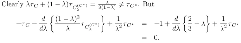
Example 4.4. Let C(u; v) = C+(u; v) = minfu; vg, and C (u; v) = C0(u; v) = uv.
Then C = 1, C = 0, C(C ) =
Clearly C+ (1 ) C(C ) = 3(1 ) 6= C . But C+ d d (1 )2 C(C ) + 1 2 C = 1 + d d 2 3+ + 1 2 C = 0:
5. Characterization and Generation of New Copulas
Investigation of the form of the complement copula functions for the indepen-dence copula given in Examples 2.2-2.5 suggests the study of the copulas of certain forms. On generating new families of copulas one of the following approaches can be followed:
Approach 1. For a preselected C , …nd C?(C )[C(C )] such that
C(u; v) = C (u; v) C?(C )(u; v) C(u; v) = 1C (u; v) + 1 1 C(C )(u; v) is a copula. In fact, Rodriguez-Lallena and Ubeda-Flores [8] consider the case where C (u; v) = uv, and C?(C )(u; v) = f (u)g(v). Lai and Xie [4] study the case for C (u; v) = uv, and C?(C )(u; v) = (u; v). Bairamov and Kotz [2] present and
dis-cuss the extension of the case C (u; v) = uv, and
C?(C )(u; v) = uvf (u)g(v) = f (u)g (v). Therefore, these results can all be seen as the special case of our setup. Another form comes from the Ali-Mikhail-Haq complement function for the independence copula, i.e., C?(u; v) =
uv + a(u)b(v)C(u; v).
The following result will help us to unify all of the work on generating new families under Approach 1.
Theorem 5.1. Let T be a targeted copula and t be the corresponding copula density function. Consider a two-place function C?(T ) such that
(i) C?(T )(0; v) = C?(T )(u; 0) = C?(T )(1; v) = C?(T )(u; 1) = 0; (ii)
@2C(T ) ? (u; v)
@u@v t(u; v)
for all u; v 2 [0; 1].
Then C(u; v) = T (u; v) C?(T )(u; v) is a copula.
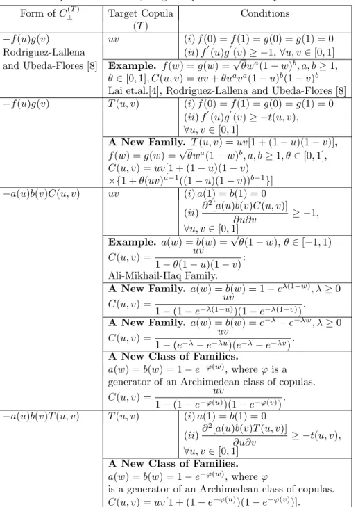
Table 2 in Appendix integrates existing results to our general setup and presents some new cases.
Approach 2. Starting with C and C, construct new families of copulas fC(C )g. Now let us look at the conditions that will make C(C )a copula. Only condition that needs to be veri…ed is the 2-increasingness. Let
v1;v2
for u1; u2; v1; v2 2 [0; 1] such that u1 u2 and v1 v2. For C(C ) to be
2-increasing, it is su¢ cient to be v1;v2 u1;u2(C )
v1;v2
u1;u2(C). In terms of copula density functions, c(u; v) = @2@u@vC(u;v), this yields c (u; v) c(u; v), 8u; v 2 [0; 1]. For the independence case this condition becomes c(u; v) 1, 8u; v 2 [0; 1].
Suppose that is a conjugate symmetric family around C . That is, if C 2 ,
then the symmetry function of C; C(C ) 2 . Therefore,
C(C )(u; v) = C(u; v; !( ; ; )). Now one can form various functional equations starting from basic de…nitions and attempt to solve them. Note that for the FGM and the Fréchet-Mardia families !( ; ; ) = 1 . For the parametrized copulas described above
C(u; v; ) + (1 )C(C )(u; v) = C (u; v; )
) C(u; v; ) + (1 )C(u; v; !( ; ; )) = C (u; v; ) ) h( ) + (1 )h(!( ; ; )) = h( )
) !( ; ; ) = h 1 h( 1) h( ) :
Therefore, if C(u; v; ) is a linear function of , then !( ; ; ) = 1 which is he case for the FGM and Fréchet-Mardia class of copulas.
Theorem 5.2. Let = fC(u; v; ) : 2 g be a conjugate symmetric family around C(u; v; ). Then C(C ) is a copula i¤ !( ; ; ) 2 .
Corollary 5.3. Let = fC(u; v; ) : 2 g be a conjugate symmetric family around C(u; v; ), and C(u; v; ) is linear in . Then, C(C )is a copula i¤ 1 2
.
Example 2.2 (Continued). For the FGM family C(C ) is a copula for
1 2 [ 1; 1].
Example 2.3 (Continued). For the Fréchet-Mardia family C(C ) is a copula for 1 11 1; 1 11 2 2 [0; 1] and 1 11 ( 1+ 2) 1.
6. Concluding Remarks
The two special functions de…ned and studied in this paper open up an alterna-tive way of understanding the behaviour of copulas. We have shown some of the properties of these functions and discussed how they can be used on generating new classes. Starting with a copula and targeting another could be a helpful tool for approximating copulas, obtaining some decompositions, and on updating starting copula in dependence model building with a new one. We will attempt to address these issues in our subsequent papers.
APPENDIX
Proof of Theorem 4.2. Proof of the theorem is tedious but straightforward which is given here.
(i) By using the alternative form of the Kendall’s tau
C= 1 4 1 Z 0 1 Z 0 @ @uC(u; v) @ @vC(u; v)dudv = 1 4 1 Z 0 1 Z 0 kC(u; v)dudv:
C(u; v) + (1 )C(C )(u; v) = C (u; v) ) @u@ C(u; v) + (1 ) @ @uC (C ) (u; v) = @u@ C (u; v) ) @u@ C(u; v) @ @vC(u; v) + (1 ) @ @uC (C ) (u; v)@v@ C(u; v) = @ @uC (u; v) @ @vC(u; v)
) kC(u; v) + (1 )@u@ C(C )(u; v)@v@ C(u; v) = 1kC (u; v)
+(1 1)@ @uC (u; v) @ @vC (C ) (u; v) ) kC(u; v) + (1 )(1 1)kC(C )(u; v) (1 1)@ @uC (C ) (u; v)@v@ C (u; v) = 1kC (u; v) + (1 1)@u@ C (u; v)@v@ C(C )(u; v)
) kC(u; v) + (1 )(1 1)kC(C )(u; v) 1kC (u; v)
= (1 1) @u@ C (u; v)@v@ C(C )(u; v) +@u@ C(C )(u; v)@v@ C (u; v) ) 21kC(u; v) + (1 )kC(C )(u; v)
1
1kC (u; v)
= @u@ C (u; v)@v@ C(C )(u; v) +@u@ C(C )(u; v)@v@ C (u; v) ) 21 1 R 0 1 R 0 kC(u; v)dudv + (1 ) 1 R 0 1 R 0 kC(C )(u; v)dudv 11 1 R 0 1 R 0 kC (u; v)dudv = 1 R 0 1 R 0 @ @uC (u; v) @ @vC (C )
) 214 1 R 0 1 R 0 kC(u; v)dudv + (1 )4 1 R 0 1 R 0 kC(C )(u; v)dudv 1 14 1 R 0 1 R 0 kC (u; v)dudv = 4 1 R 0 1 R 0 @ @uC (u; v) @ @vC (C )
(u; v) +@u@ C(C )(u; v)@v@ C (u; v) dudv ) 1 2 4 1 R 0 1 R 0 kC(u; v)dudv (1 )4 1 R 0 1 R 0 kC(C )(u; v)dudv 114 1 R 0 1 R 0 kC (u; v)dudv = 4 1 R 0 1 R 0 @ @uC (u; v) @ @vC (C )
(u; v) +@u@ C(C )(u; v)@v@ C (u; v) dudv ) 1 2 1 1 + 4 1 R 0 1 R 0 kC(u; v)dudv (1 ) 1 1 + 4 1 R 0 1 R 0 kC(C )(u; v)dudv 1 1 1 1 + 4 1 R 0 1 R 0 kC (u; v)dudv = 4 1 R 0 1 R 0 @ @uC (u; v) @ @vC (C ) (u; v) + @ @uC (C ) (u; v)@ @vC (u; v) dudv ) 1 2 (1 C) (1 )(1 C(C )) 1 1 (1 C ) = 4 1 R 0 1 R 0 @ @uC (u; v) @ @vC (C )
(u; v) +@u@ C(C )(u; v)@v@ C (u; v) dudv If C(C )and C are symmetric, then letting u = v and v = u, we end up with
) 2 1 (1 C) (1 )(1 C(C )) 1 1 (1 C ) = 8 1 Z 0 1 Z 0 @ @uC (u; v) @ @vC (C ) (u; v)dudv ) 2 1 (1 C) (1 )(1 C(C )) + 1 1 (1 C ) = 8 1 1 Z 0 1 Z 0 @ @uC (u; v) @ @vC(u; v)dudv ) (1 C) (1 )2 (1 C(C )) + 1 (1 C ) = 8 1 Z 0 1 Z 0 @ @uC (u; v) @ @vC(u; v)dudv: By taking the derivatives of both sides with respect to ,
) 1 C dd n (1 )2 (1 C(C )) o 1 2(1 C ) = 0 ) 1 C 2 1 2 (1 C(C )) (1 ) 2h d d C(C ) i 1 2(1 C ) = 0 ) 2 2 C ( 2 1)(1 C(C )) (1 )2 h d d C(C ) i (1 C ) = 0 ) 2 2 C ( 2 1) + ( 2 1) C(C ) (1 )2 h d d C(C ) i (1 C ) = 0 ) 2 C+ ( 2 1) C(C ) (1 )2 h d d C(C ) i + C = 0:
(ii) Given C+ (1 ) C(C ) = C , we have
) 2 44 1 Z 0 1 Z 0 C(u; v)dC(u; v) 1 3 5 + (1 ) 2 44 1 Z 0 1 Z 0 C(C )(u; v)dC(C )(u; v) 1 3 5 = 4 1 Z 0 1 Z 0 C (u; v)dC (u; v) 1 ) 1 Z 0 1 Z 0 C(u; v)dC(u; v) + (1 ) 1 Z 0 1 Z 0 C(C )(u; v)dC(C )(u; v) = 1 Z 0 1 Z 0 C (u; v)dC (u; v):
We will drop the arguments of the functions to have an easier-to-understand ex-pression. ) 1 Z 0 1 Z 0 CdC + (1 ) 1 Z 0 1 Z 0 C(C )dC(C )= 1 Z 0 1 Z 0 C dC ) 1 Z 0 1 Z 0 CdC + (1 ) 1 Z 0 1 Z 0 1 1 C 1 C d 1 1 C 1 C = 1 Z 0 1 Z 0 C dC
) 1 Z 0 1 Z 0 CdC + 1 1 1 Z 0 1 Z 0 [C C] d [C C] = 1 Z 0 1 Z 0 C dC ) 1 Z 0 1 Z 0 CdC + 1 1 1 Z 0 1 Z 0 C dC C dC CdC + 2CdC = 1 Z 0 1 Z 0 C dC ) 1 1 Z 0 1 Z 0 CdC 1 1 Z 0 1 Z 0 [C dC + CdC ] = 1 1 Z 0 1 Z 0 C dC ) 1 Z 0 1 Z 0 CdC 1 Z 0 1 Z 0 [C dC + CdC ] = 1 Z 0 1 Z 0 C dC ) 1 Z 0 1 Z 0 [C C ] dC = 1 Z 0 1 Z 0 [C C ] dC : Similarly, 1 Z 0 1 Z 0 [C C ] dC = 1 Z 0 1 Z 0 [C C ] dC ) C+ (1 ) C(C ) = C :
Table 2. Complement Function, Target Copula and Necessary Conditions.
Form of C?(T ) Target Copula Conditions
(T )
f (u)g(v) uv (i) f (0) = f (1) = g(0) = g(1) = 0
Rodriguez-Lallena (ii) f0(u)g0(v) 1; 8u; v 2 [0; 1] and Ubeda-Flores [8] Example. f (w) = g(w) =p wa(1 w)b; a; b 1;
2 [0; 1]; C(u; v) = uv + uava(1 u)b(1 v)b
Lai et.al.[4], Rodriguez-Lallena and Ubeda-Flores [8] f (u)g(v) T (u; v) (i) f (0) = f (1) = g(0) = g(1) = 0
(ii) f0(u)g0(v) t(u; v); 8u; v 2 [0; 1]
A New Family. T (u; v) = uv[1 + (1 u)(1 v)], f (w) = g(w) =p wa(1 w)b; a; b 1; 2 [0; 1];
C(u; v) = uv[1 + (1 u)(1 v) f1 + (uv)a 1((1 u)(1 v))b 1g]
a(u)b(v)C(u; v) uv (i) a(1) = b(1) = 0
(ii)@ 2[a(u)b(v)C(u; v)] @u@v 1; 8u; v 2 [0; 1] Example. a(w) = b(w) =p (1 w); 2 [ 1; 1) C(u; v) = uv 1 (1 u)(1 v): Ali-Mikhail-Haq Family.
A New Family. a(w) = b(w) = 1 e (1 w); 0
C(u; v) = uv
1 (1 e (1 u))(1 e (1 v)):
A New Family. a(w) = b(w) = e e w; 0
C(u; v) = uv
1 (e e u)(e e v):
A New Class of Families.
a(w) = b(w) = 1 e '(w), where ' is a generator of an Archimedean class of copulas.
C(u; v) = uv
1 (1 e '(u))(1 e '(v)):
a(u)b(v)T (u; v) T (u; v) (i) a(1) = b(1) = 0 (ii)@
2[a(u)b(v)T (u; v)]
@u@v t(u; v);
8u; v 2 [0; 1] A New Class of Families. a(w) = b(w) = 1 e '(w), where '
is a generator of an Archimedean class of copulas. C(u; v) = uv[1 + (1 e '(u))(1 e '(v))]:
Özet. Bu çal¬¸smada, bir kapula verildi¼ginde bir ba¸ska kapula he-de‡enmekte ve çe¸sitli iki yerli fonksiyonlar kullan¬larak bu iki ka-pulan¬n ba¼glanmas¬na giri¸silmektedir. Çal¬¸smada bu tür fonksi-yonlardan ikisi, simetri ve tümleyen fonksiyonlar tan¬mlanm¬¸s ve incelenmi¸stir.
References
[1] Amblard, C., Girard, S. (2005), Symmetry and dependence properties within a semiparametric family of bivariate copulas, Nonparametric Statistics, 14(6), 715-727.
[2] Bairamov, I., Kotz, S. (2002), Dependence structure and symmetry of Huang-Kotz FGM distributions and their extensions, Metrika, 56, 55-72.
[3] Esary, J.D., Proschan, F. (1972), Relationships among some concepts of bivariate dependence, Ann. Math. Statist., 43, 651-655.
[4] Lai, C.D., Xie, M. (2000), Anew family of positive quadrant dependent bivariate distributions, Statist. Probab. Lett., 46, 359-364.
[5] Lehmann, E.L. (1966), Some concepts of dependence, Ann. Math. Statist., 37, 1137-1153. [6] Nelsen, R.B. (1998), Concordance and Gini’s measure of association, Nonparametric Statistics,
9, 227-238.
[7] Nelsen, R.B. (1999), An Introduction of Copulas, Springer, New York.
[8] Rodriguez-Lallena, J.A, Ubeda-Flores, M. (2004), Anew class of bivariate copulas, Statist. Probab. Lett., 66, 315-325.
[9] Sungur, E.A. (2005), Some observations on copula regression functions, Commun. Stat. Theor. Methods, 34, 1967-1978.
Current address :1Division of Science and Mathematics, University of Minnesota-Morris,
Mor-ris, MN, 56267, USA, 2Gazi Üni. Fen-Edebiyat Fak., ·Istatistik Bölümü, 06503, Teknikokullar,
Ankara, Türkiye