Message-passing based algorithm for the global alignment of clustered pairwise PPI networks

KADIR HAS UNIVERSITY

GRADUATE SCHOOL OF SCIENCE AND ENGINERRING

MESSAGE-PASSING BASED ALGORITHM FOR THE GLOBAL

ALIGNMENT OF CLUSTERED PAIRWISE PPI NETWORKS

GRADUATE THESIS

DOĞAN YİĞİT YENİGÜN

D oğa n Y iği t Y eni gün M .S . T he si s 2013

MESSAGE-PASSING BASED ALGORITHM FOR THE GLOBAL

ALIGNMENT OF CLUSTERED PAIRWISE PPI NETWORKS

DOĞAN YİĞİT YENİGÜN

Submitted to the Gradute School of Science and Engineering in partial fulfillment of the requirements for the degree of

Master of Science in

COMPUTER ENGINEERING

KADIR HAS UNIVERSITY December, 2013

vi

ABSTRACT

MESSAGE-PASSING BASED ALGORITHM FOR THE GLOBAL ALIGNMENT OF CLUSTERED PAIRWISE PPI NETWORKS

Doğan Yiğit Yenigün

Master of Science in Computer Engineering Advisor: Assoc. Prof. Cesim Erten

December, 2013

Constrained global network alignments on pairwise protein-protein interaction (PPI) networks involve matchings between two organisms where proteins are grouped together in a great number of clusters, produced by algorithms that seek functionally ortholog ones and these organisms are represented as graphs. Unlike balanced global network alignments (GNA), this has not gained much popularity in bioinformatics. Only a few methods have been proposed thus far; by assuming specific structures of networks including the clusters themselves and the density of the PPI networks are not too large, then optimal alignments can be encountered. Here, we introduce a general-purpose algorithm that is able to work on any kind of graph structures while taking advantage of the message-passing method, based on propagation between clusters. When these graphs satisfy conditions like continuous interaction connectivity of proteins across all neighbored clusters, in addition to previous explanations, the optimality of alignments can still be achieved. Convergence of the cluster network can occur at the point where the maximum number of conserved interactions are detected. Many experiments were made with balanced GNA algorithms and our algorithm may find more conservations and more importantly, alignments have higher biological quality than other ones in various instances.

vii

ÖZET

KÜMELENMİŞ İKİLİ PROTEİN-PROTEİN ETKİLEŞİM AĞLARININ GLOBAL HİZALANMASI İÇİN MESAJ VERMEYE DAYALI ALGORİTMA

Doğan Yiğit Yenigün

Bilgisayar Mühendisliği, Yüksek Lisans Danışman: Doç. Dr. Cesim Erten

Aralık, 2013

İkili protein-protein etkileşim ağları üzerinde kısıtlanmış global ağ hizalaması, işlevsel olarak ortak proteinleri arayan algoritmalar tarafından üretilen çok sayıdaki küme içerisinde gruplanmış olan iki organizmanın proteinleri arasında en iyi eşleşmeleri içerir ve bu organizmalar graph yapısı olarak gösterilirler. Dengeli global ağ hizalamanın aksine biyoenformatik alanında fazla popülerlik kazanmamıştır. Şu ana kadar sadece birkaç yöntem önerilmiştir; kümelerin kendileri de dahil özel ağ yapıları ve protein-protein etkileşim ağlarının yoğunluğunun çok büyük olmadığı varsayılırsa, en iyi hizalamalarla karşılaşılabilir. Burada, her tür graph yapısı üzerinde çalışabilen ve kümeler arasında yayılıma dayalı mesaj verme yönteminden faydalanan genel amaçlı bir algoritmayı sunuyoruz. Bu graphlar önceki varsayımlarla beraber birbirine komşu tüm kümeler boyunca proteinlerin devamlı etkileşim bağlantıları olması gibi koşulları sağlarlarsa, hizalamaların en iyisine halen ulaşılabilir. En çok sayıda korunmuş etkileşimlerin bulunduğu noktada küme ağının yakınsaması meydana gelebilir. Dengeli global ağ hizalama algoritmaları ile birçok deney yapılmıştır ve bizim algoritmamız diğerlerinden daha fazla korunmuş etkileşimi bulabilir ve daha da önemlisi, değişik örneklerde hizalamalar daha yüksek biyolojik kaliteye sahip olabilir.

viii

Acknowledgements

I, hereby, thank my thesis instructor, Assoc. Prof. Cesim Erten, for the advices of thesis progression, the proposals of methods, approaches in development of the algorithm and the meetings we have made for disscusions. This thesis is in collaboration with TÜBİTAK project, BionetAlign: Global Alignments with the Intention of Functional Orthology Mining in Biochemical Networks, conducted by himself.

ix

Table of Contents

2.2 The Cluster Network... 8

2.2.1 Cluster Nodes... 8

2.2.2 Cluster Edges... 10

2.2.3 Cluster Permutations... 12

2.3 Conserved Interactions Within Clusters... 14

2.4 Plausible Edge Counts... 17

2.5 The Message-Passing Method... 19

2.5.1 Our Formation and Vision of Message-Passing... 19

2.5.2 Functions of the Message-Passing, External Conservations and Output... 21

2.5.3 Deatiled Analysis and Claims... 27

2.5.4 Discussions for Convergence... 34

2.6 The Whole Algorithm Pseudocode... 36

3 Experiments and Results 39 3.1 Comparisons with Algorithms... 39

x

3.1.1 Evaluation of Conserved Interactions... 42

3.1.2 Runtime Performances... 45

3.1.3 Discussion of Our Algorithm Runtime Determinants... 47

3.2 Biological Significance... 48

Conclusion 52

xi

List of Tables

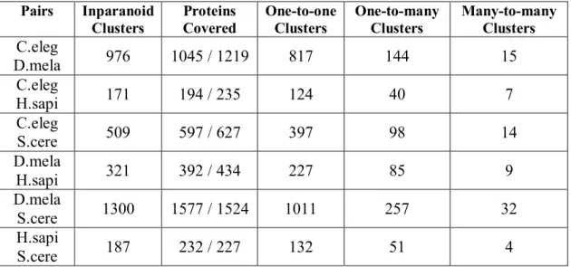
Table 3.1 Results of the clusterization made by Inparanoid... 41

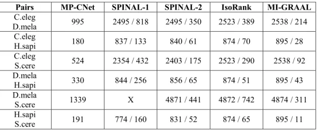
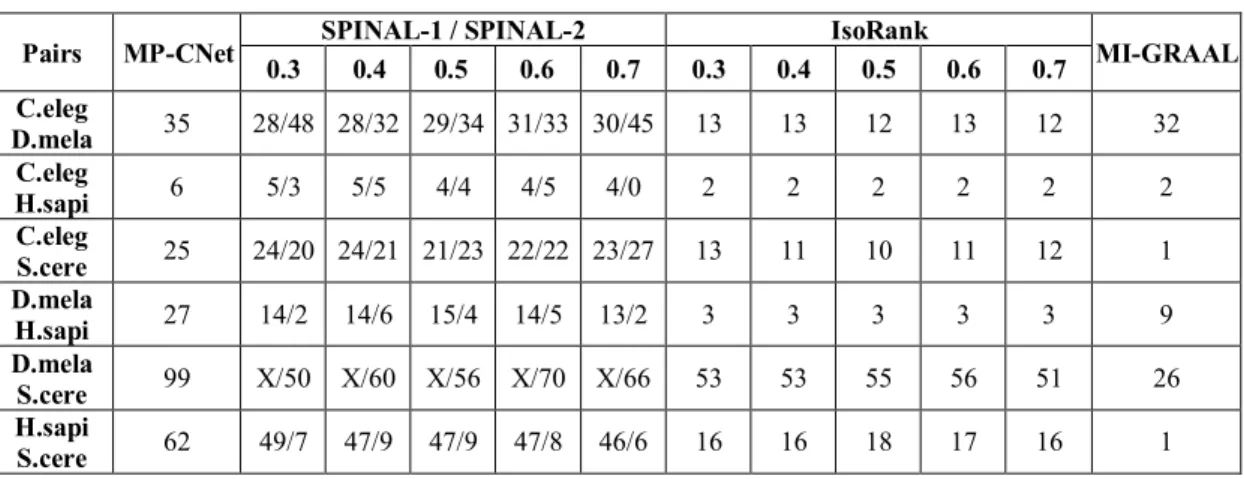
Table 3.2 Number of matches of alignments generated by algorithms... 43

Table 3.3 Number of total conserved interactions extracted by algorithms... 44

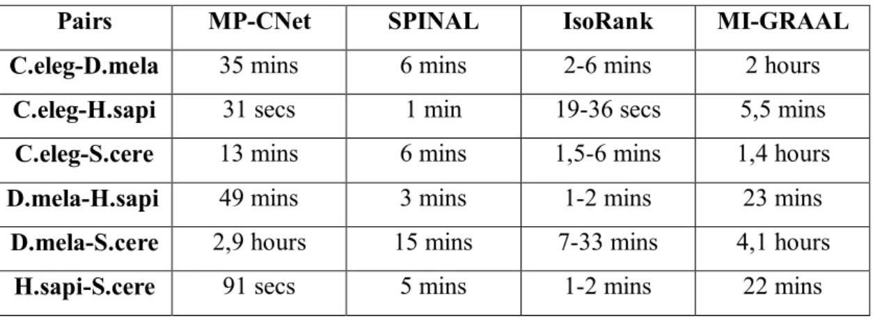
Table 3.4 Total runtime of the algorithms against all instances... 46

Table 3.5 GO consistency scores of all alignments by algorithms (unfiltered)... 50

xii

List of Figures

Figure 2.1 An illustration of the addition of cluster edges... 11

Figure 2.2 An example of all available permutations of a cluster... 13

Figure 2.3 A demonstration of internal conserved interactions (fixed scores) search for some permutations... 16

Figure 2.4 Counting pluasible edges of a cluster permutation... 18

Figure 2.5 An example of external conserved interaction (edge score) between clusters... 24

xiii

List of Symbols

α : The control parameter

: Unit fixed score

: Unit edge score

: Cluster permutations

xiv

List of Abbreviations

PPI : Protein-protein Interaction

GNA : Global Network Alignment

LNA : Local Network Alignment

MP-CNet : Message-Passing on the Clustered Network

SPINAL : Scalable Protein Interaction Network Alignment

MI-GRAAL : Matching-based Integrative Graph Aligner

DIP : Database of Interacting Proteins

1

Chapter 1

Introduction

Thanks to the fast growth of available biological data for several decades, in parallel, many computational methods and approaches have been produced over time, paving the way for uncovering interactions and recognizing patterns biologically between organisms as they play an important role in bioinformatics. High-throughput techniques like yeast two-hybrid system (Fields and Songs, 1989; Finley and Brent, 1994; Sato et al., 1994; Ito et al., 2001) and co-immunoprecipitation unified with mass spectrometry (Aebersold and Mann, 2003) have contributed to the presence of such data, particularly various species, by a significant proportion.

In recent years, protein-protein interaction (PPI) network alignments, which are the most noticeable type of data accepted by many researchers, are studied for observing the similarities in terms of pathways, homologies and functions between pairs of species. The set of instructions running on network data for the analysis are network alignment algorithms. The general aim is to create the best alignment as large and accurate as possible based on given two or more PPI networks from different species. For supplying easiness to these algorithms, these kind of networks can be represented as graphs in terms of data structure where proteins are nodes and interactions between proteins are edges. This is the most convenient way to perform

2

measurements on PPI networks because recent algorithms have been designed to work on graph structures and make one-to-one matchings, hence these are comprehended like graph matching algorithms. Additionally, any other materials may be included as input data (e.g. sequence similarity of proteins) for smoother and more accurate alignments.

In general term, they can be categorized in two main groups: Local network alignment (LNA) algorithms identify subnetworks of different species that match closely to each other in terms of network topology and/or other variables. The first known algorithm of this type is PathBLAST (Kelley et al., 2003, 2004) that enforces the BLAST algorithm (Altschul et al., 1990) for searching the high-scoring local alignments between PPI networks. Sharan et al. (2005) extends the idea with NetworkBLAST to include multiple species. MaWISh (Koyutürk et al., 2006) adapts to the duplication and elimination models inspired by biological events to perform local alignment. Graemlin (Flannick et al., 2006) takes advantage of conserved functional modules of networks. Global network alignment (GNA) algorithms, on the other hand, take PPI networks as a whole and provide one-to-one matches across all proteins. IsoRank (Singh et al., 2007) is known to be the first algorithm to make alignment globally on pairwise PPI networks, using eigenvalue formulation. Later, the algorithm was expanded to work on multiple networks as well (Singh et al., 2008) and so with IsoRankN (Liao et al., 2009). Graemlin was later modified to generate global alignments beyond pairwise networks, examining phylogenetic relationships (Flannick et al., 2008). PATH algorithm (Zaslavskiy et al, 2009a) adapts to convex-concave relaxation approach to find a solution path over the pairwise networks. PISwap (Chindelevitch et al., 2010) first performs the global alignment by sequence data, then necessary changes are made by benefiting from

3

network topology. MI-GRAAL (Kuchaiev and Przulj, 2011) constructs the alignment by integration and several different sources of protein similarity, and was demonstrated to outperform other variants such as H-GRAAL (Milenkovic et al., 2010) and GRAAL (Kuchaiev et al., 2010). The last known state-of-the-art algorithm of global alignment is SPINAL (Aladag and Erten, 2013) which consists of two stages; first estimating alignment scores, then resolving conflicts to enhance the alignment while also dealing with scalability issues. Additionally, SubMAP has been proposed (Ay et al., 2011) that has the capability of making one-to-many mappings of proteins.

LNA methods are able to expose more than one region of matches between networks, i.e. local matchings provide specific areas of interactions amongst these network of proteins. However, GNA looks for comprehensive matchings by taking into account all proteins and attempts to align them. This gives the best conserved functions as much as possible. By the aspect of computation, GNA is more difficult than LNA because one protein in a network is sought to match with a protein of the other network that achieves the highest optimality, although it is desirable for many algorithms to detect functional orthologs. In addition, most of GNA algorithms are allowed to use weights between the network topology and protein sequence similarities (denoted with or ) in order to perform the alignment. This gives rise to number of different alignments and flexibility to the output. Algoritms that accept such a control parameter are generally classified as balanced GNA algorithms.

Another issue of network alignment is intractability in terms of computation, when networks are getting too dense. This causes alignments to become distant from exactness. Furthermore, there is no algorithm to work in polynomial time for the problem (Zaslavskiy et al., 2009b) as the current algorithms endavours to make the

4

best approximate results by impliying heuristic methods but with NP-hardness (Klau, 2009; Aladag and Erten, 2013).

While on the research of identification of protein interactions across species especially before network alignment algorithms were produced widely, some questions have been arisen such as which proteins or genes are in common with those from other species (i.e. orthologs), and which provide shared biological functions against their ancestors or familiar organisms. For this approach, Inparanoid (Remm et al., 2001), HomoloGene and OrthoMCL (Li et al., 2003) have been proposed to disambiguate functionally ortholog proteins by grouping them in clusters after specific methods are implemented based on the algorithms. By using the information of finite number of clusters as well as covered proteins, the whole can be interpreted as a separate network, i.e. the cluster network and necessary connections are carried out between those with specific regulations; for example, conservation of functions in proteins of pairwise PPI networks for any two clusters. This kind of study is usually referred to constrained GNA problem, where proteins are restricted to match with the others solely in the same clustered group and attempts to create an alignment in this way. This may help reduce the intractability issue of the networks and perhaps holding functionally ortholog proteins together may bring more potentials for similar properties.

To the best of our knowledge, there are not much studies so far involving the solution of this problem. Bandyopadhyay et al. (2006) investigated the proteins between Drosophila melanogaster and Saccharomyces cerevisiae to identify functionally orthologs using Markov random field (MRF) methods while these are constrained to belong to the respective clusters, produced by Inparanoid algorithm. Another noteworthy procedure is the message-passing algorithm by Zaslavskiy et al.

5

(2009b), that is able to align the networks optimally with meesage-passing on particular clustered structure of proteins assuming if the network is sparse. Here, message-passing is a form of communication where objects send and receive messages to each other. A special variant, belief propagation (BP) has been introduced (Pearl, 1982) to make inferences on graphical models (e.g. Bayeisan networks and Markov random fields) and included in many applications, for instance, artificial intelligence (Pearl, 1988), statistics (Lauritzen, 1996), low-density parity-check codes and any other areas with experimental successes (Horn, 1999; Aji and McEliece, 2000; Yedidia et al., 2000).

In this paper, we propose a new algorithm, called MP-CNet which is the abbreviation of Message-Passing on the Clustered Network, to execute on constrained GNA problem and it attempts to find the best alignment with as many as conservations of proteins on clustered pairwise PPI networks with BP-based message passing method, possessing some ideas of Zaslavskiy et al. (2009b). Here, clusters propagate their best matches to their neighbors in order to increase the overall amount of conserved interactions and the whole cluster network converges at a point when the maximum amount is reached. Our contribution is that we show a general-purpose algorithm with the implementation of message-passing can be used on any kind of cluster network structure including the PPI networks themselves. The methods, in some cases, have resemblances with the implementation of maximum weight bipartite matching, but are not complicated at all. Also, by checking the capabilities with other algorithms, we draw attention to the situations that our algorithm can reveal larger number of conserved interactions if filterings are applied to other alignments and highlight that it can provide higher quality of biological impacts than existing algorithms.

6

The rest of the paper is organized as follows. In section 2, we highly detail working principles of MP-CNet by explaining the definition of the problem to solve, data processing stages, any procedures, approaches involved in the message-passing method through the subsections. In addition, the algorithm progession and claims of optimal alignments are elaborated. In section 3, we compare our algorithm to other global alignment algorithms that approaches the problem as balanced, by the aspect of number of found conserved interactions, running performances and general biological quality of the alignments. In Conclusion section, important remarks and final discussions are made, in additon to any future plans for further improvements.

7

Chapter 2

Methods and The Message-Passing Algorithm

2.1. Problem Definition

Our algorithm, MP-CNet, is designed to work on pairwise protein-protein interaction networks. We denote = ( , ) and = ( , ) as two undirected graphs which are the PPI networks of two different species. = { , … , } and = {ℎ , … , ℎ } are the finite set of nodes of their respective graphs, each representing the proteins of PPI networks. ⊂ × and ⊂ × are the edges of these graphs which corresponds to the interactions between proteins. We assume there are no any self-loops i.e., ( , ) ∉ and (ℎ , ℎ ) ∉ . In addition, we are given a set of disjoint clusters = { , … , } such that each consists of a subset of nodes of and a subset of nodes of .

Here, a pair of node mappings ( , ℎ ), ( , ℎ ) provide a conserved interaction if ( , ) ∈ and (ℎ , ℎ ) ∈ . Given the two graphs and together with the set of clusters , we define the constrained global network alignment (GNA) problem that of finding a one-to-one mapping that satisfies the constraints; that is, each mapped pair belongs to the same cluster ∈ and that maximizes number of conserved interactions. Before discussing the algorithm in detail, we highlight the main processes involved in preparing the input data.

8 2.2. The Cluster Network

The construction of the cluster network is the first major part of processing the input data. This network itself can be thought of as a separate graph but has a correlation with the PPI network graphs in accordance with the clusterization of nodes. For this purpose, we denote be the cluster graph (network) which will be substantially used by MP-CNet in many stages. Of course, like the PPI network graphs, we denote = { , … , } to represent the finite number of disjoint clusters and ⊂ × are the finite set of edges of the cluster graph. In the initialization, remains empty. We first describe how the cluster set is constructed and the corresponding vertex set of .

2.2.1. Cluster Nodes

For the generation of , we benefit from Inparanoid algorithm (Remm et al., 2001) which is known to exhibit a good overall balance by both sensitivity and specificity (Chen et al., 2007). Mentioning briefly, Inparanoid automatically detects orthologs and in-paralogs between any given two species and uses special techniques for revealing the clusters. From the definition, ortholog proteins are that evolve directly from a single species from the last common ancestor and have a high proportion to share function. Paralog ones are homologs that contain uncertainty of functional equivalence between the orthologs which are derived from a single ancestor at the speciation event. It is also noted that paralogs can be arisen from duplication event before speciation is occured. For this reason, paralogs are split into two types: In-paralogs are the ones that are duplicated after the speciation as they are considered to be orthologs. Those preceding the speciation are denoted as

out-9

paralogs and they are not counted orthologs. In this context, Inparanoid algorithm does not include out-paralogs in the output.

There are many parameters available in the algorithm which can affect the placement of proteins (i.e. the orthologs) into clusters, thus the whole general output. The most notable one is pairwise similarity score and this is where the orthology detection begins by computing all similarity scores between all existing protein sequences of two species. It is measured by another program called BLAST (Altschul et al., 1990) to create E-values for all possible pairs of proteins from pairwise species. These values are helpful to determine the orthologs and clusters afterwards. Furthermore, a score cut-off is required to distinguish the scores from spurious ones, i.e. any cluster whose score is less than the cut-off will not be included in the output. Overlap cut-off is also used to determine the ratio that the matching protein of the longer sequence must surpass its total length. In-paralog confidence values, bootstrapping for ortholog groups and coverage cut-off are the other countable essential parameters. The output consist of cluster number, its score and proteins from the PPI networks in the related cluster.

The rest of the details of the algorithm are out of the scope of this paper (for more details, see Remm et al., 2001). We only focus on the results (i.e. the set of clusters), generated by Inparanoid and mainly, MP-CNet uses it as a guide to produce the clusters and place the appropriate proteins into them correctly. Only the cluster number and its proteins are needed for generating the clusters. It can be seen that clusters with higher scores are likely to be at the top of the clustering information. However, it is not necessary to be in order, though it helps to become organized and understand them better.

10

When we look at each cluster, three specific kinds can be encountered: One-to-one clusters contain only One-to-one node (protein) from both graphs. In other words, the single node from graph in this cluster can merely match one node from graph , leaving no other option to match from outside. One-to-many clusters have one node from graph and more than one nodes from graph and vice versa. However, there is still one match that can really occur. For many-to-many clusters, more than one nodes from both graphs are involved. The amount of matches in that kind of cluster is the same with whose number of nodes in the respective graph is less. At the time of the creation of each cluster node , it is recognizable that not every one of them cover the same number of nodes from both graphs. This especially happens for all one-to-many and some many-to-many clusters. To address this issue, we insert dummy nodes (i.e. artificial nodes) to whichever the number of subset of or nodes is smaller in the cluster node and they have no edges in their respective PPI-network graphs. The main reason for ensuring the equalization to each cluster is to simplify the algorithm description and implementation details, and this allows every nodes to be matched, although those with dummy nodes are not included in the output. Namely, it must not be perceived such that we do not equalize the number of nodes between graphs and ; we just perform this on clusters which needs to be equalized by getting the number of 'real' nodes contained. Consequently, ∀ ∈ has the same total number of nodes covered from both graphs and we denote

= {( , … , ), (ℎ , … , ℎ )} where , … , ∈ and ℎ , … , ℎ ∈ . 2.2.2. Cluster Edges

After preparing all cluster nodes, we perform a check on each cluster to observe if it can make connections to other clusters and so, these connections will be interpreted as cluster edges (added into ) for our cluster graph.

11

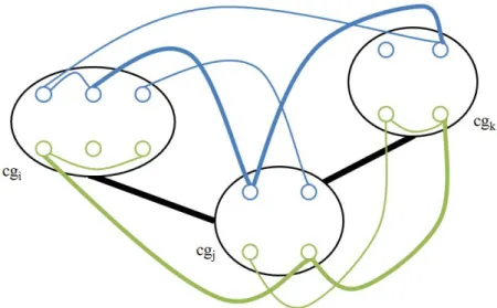
This process is straightforward. We take every possible combination of cluster pairs, that is, , ∈ and 1 ≤ < , < ≤ , every ( , ) pairs are investigated. For any pair, we start from the subset of nodes of of cluster nodes and ( { , … , } ∈ and { , … , } ∈ ) to compare them with all available edges from for an existence of at least one edge, involving these nodes. Next, we advance to make the similar comparison with the subset of nodes of of these clusters to the graph edges of . That is, we perform this with {ℎ , … , ℎ } ∈ and {ℎ , … , ℎ } ∈ to all edges from . If such edges are found for both sides, then it is safe to add a connection between these cluster nodes and included in . This goes on like this until every combination of cluster node pairs are examined. Note that in Figure 2.1, an edge between and is not formed because there is no edge available in that involves one node from the subsets of of and . As a result, the construction of our cluster graph is finally completed.

Figure 2.1 An illustration of the addition of cluster edges . Blue and green components represent nodes and edges of graph and , respectively. Here, bold

12

The structure of is vital for MP-CNet because it will be used every time in the oncoming stages and so the finding of conserved interactions between cluster nodes. The structure can be in any form such that there may be many cluster nodes having one or more connections (sometimes called adjacents or neighbors) to any other; lots of small or a large group of joint networks. In the meantime, the number of cluster edges can vary, depending on the number of cluster nodes, number of covered nodes in clusters ∀ ∈ and the edges of and . Note that more connections among all existing cluster nodes allow to get more conserved interactions.

2.2.3. Cluster Permutations

We have presented an easiness to our algorithm by adding dummy nodes to the necessary clusters to make the number of subset of nodes from and equal. Now, we would like to extract how many different varieties of matches could be carried out for all clusters. For this reason, the creation of permutations begins when construction of is finished.

Let be the permutation space, containing all possible permutations of ∀ ∈ , a multi-dimensional variable. Also, let ( ) be the permutations of . Here, in this process, one-to-one and many-to-many clusters are used, since all one-to-many clusters are converted to many-to-many by the insertion of dummy nodes to them. We assume ∀ , these permutations are derived from the subset of nodes of , while fixing the subset of nodes. This is not limited to this shape and one can make by using the appropriate nodes, too. However, this requires a comprehensive redesign to our algorithm for further steps to provide full compatibility. Hence, from the rest of the paper on, we comply that the permutations remain with subset of nodes of at all times.

13

For any cluster , its subset of nodes of are taken and sent out to a special function to generate the permutations. We follow the permutation-without-repetiton rule, so these permutations are distinctive from each other when generated. There is another variable, , which holds the current iteration of nodes to check if it is a permutation candidate to be added to not. In the intial step, first node is placed to , then a second one and so on like a stack. We actualize the examination of duplication when contains more than one node and less than , which is the maximum number of nodes can be together, and the checks are happened in every addition. For the group of nodes in at any time, we first treat them like they form a permutation and continue to add nodes up to if there is no duplication occured within all nodes inside, otherwise the last added node is removed (i.e. popped back) from and the next one is placed. When the number of nodes in is reached to , we ensure that every node is different from each other, therefore it is secure to mark them as a permutation of and included in ( ), then certainly to (Figure 2.2). This goes on until all the subset of nodes of from cluster nodes are taken care of.

Figure 2.2 An example of all available permutations of a cluster. Note that the cluster has 3 nodes from and 3! = 6 different permutations were generated.

14

A cluster has ! amount of permutations, similarly what we have said previously, where is the number of subset of nodes covered in . They are always stored till the completion of MP-CNet. Like the cluster edges of , the permutation space is important. In the next stages and even in the message-passing process for the conserved interactions, we always iterate through permutations.

2.3. Conserved Interactions Within Clusters

The stages from now on until the message-passing derive the second major part of input data processing. Here, we attempt to uncover the conserved interactions for all clusters internally and the first usage of permutation space take place for this purpose. Any found conserved interactions here can make a small contribution to the optimal alignment; that is, such a permutation of a cluster with internal conserved interactions is likely to be selected as the best although it is not always guaranteed. Because there could be another permutation in that cluster whose, for example, amount of external conserved interactions is higher then others with only internal ones, where this alteration of selection is happened in the message-passing. This will be discussed in Section 2.5. All in all, finding this kind of interactions in clusters is an important property for all permutations as an indicator of their capabilities.

We first denote ℱ to keep the number of internal conserved interactions found for all permutations of any cluster ∈ ; along with this, ( ) represents amount of found internal ones for all its permutations ( ) ∈ ( ) where 1 ≤ ≤ !. Mostly, we call this value as permutation fixed score or permutation intra-cluster score. The main reason why we name them in this shape is because we normally allow the user in MP-CNet to enter a unit score for each internal conserved interactions discovered, denoted with and more importantly, these values are held

15

as constant for use in other stages, especially in the message-passing. For easy understanding to the rest of the paper, we always treat them like a fixed score.

For any cluster node , it is not required to utilize the cluster edges. Only the matches which the permutation ( ) creates and the edges from and are needed. Note that the edges connected within could provide fixed scores. As a side note, meanwhile, we demonstrate these matches for any cluster permutation like this: for { , , … , } ∈ and ℎ , ℎ , … , ℎ ∈ , in first permutation ( ) , for instance, the matches are made as follows: ( , ℎ ) , ( , ℎ ) ,…, ( , ℎ ) . The similar production of matches are applied to the forthcoming permutations but with the necessary alterations for which subset of nodes from are matched against the subset of nodes from as the node order of ( ) states. So, the last permutation is the completely reversed one of the first and its matches go like in this shape: ( , ℎ ), , ℎ ,…, ( , ℎ ). From these descriptions we have explained thus far, a permutation can have amount of matches, which is also the same with the number of subset of nodes covered from and . In addition, ( ( − 1) / 2) number of different pairs of matches can be selected.

The computation of conserved incteractions within clusters is simple. In any

cluster ∈ , we initally choose a pair of matches

( , ) = [( , ℎ ), ( , ℎ )] that are made within the permutation ( ) ∈ ( ), and 1 ≤ < , < ≤ . Here, and are taken to search for the existence of an edge in . Then, we are ready to move on to search for ℎ and ℎ by scanning all edges of , if such an edge is available from . Otherwise, we pass on to the next possible pair of matches, as it is certain the previous one does not have the opportunity to make a internal conservation. To sum it up for this process, fixed score of a cluster permutation ( ) increases by the value of if and only if

16

( , ) and (ℎ , ℎ ) of selected pair of matches from the subset of nodes of and enclose an identical edge from and , respectively (Figure 2.3). At the end, the score is placed to ( ) and to ℱ when completed ∀ ( ). It can be also noted that a permutation can have a maximum fixed score of ( × ) which could be feasible whether the subset of nodes of that cluster mold complete subgraphs. Later, we check which permutation(s) possesses the best fixed score for each cluster by creating a list variable ℱ ℬ , for this purpose. It is necessary to keep the best permutations for comparison with another list variable, which is mentioned in Section 2.4 for getting our algorithm ready for message-passing. Here, in any cluster , fixed score of every permutation is checked and the best ones are added to

( ) ⊂ ℱ ℬ.

Figure 2.3 A demonstration of internal conserved interactions (fixed scores) for some permutations from ( ) for = 1.0.

It is admissible that one-to-one clusters cannot have fixed scores, due to having only one match and a single node from and as its subset. Hence, they are directly skipped by our algorithm. For some many-to-many clusters which were normally one-to-many clusters, all of them, but converted to that type by the addition of dummy nodes, we do not expect any fixed scores again, although they are

17

permitted to be searched. So, it shows that only the 'real' many-to-many clusters have the capability to include fixed scores for their permutations.

2.4. Plausible Edge Counts

After the preparation of permutation fixed scores for all clusters, additionally we apply a heuristic approach to measure the number of occurences in edges of and for the covered subset of nodes ∀ ∈ . This may give a clue for the permutation ( ) , having a greater number of edges that their subset of nodes existed in the edges of and respectively, brings more potential to extract many conserved interactions, so it is likely to be chosen as the best permutation in that cluster. It should be noted that every kind of edges of and are searched, including those within clusters or going from one cluster to another and no matter the cluster has neighbors or not. We denote ℰ on this objective to store the edge counts of all cluster nodes and an extra sub-dimension ( ) ⊂ ℰ for all permutations of . These values are merely used in this step and together with the fixed scores ℱ we have gathered previously, the best permutations are decided initially for getting ready MP-CNet to the message-passing stage.

In any cluster , the matches of permutation ( ) are taken one by one as they are shown with, for instance, ( ( ( ))) = ( , ℎ ) where 1 ≤ ≤ . We begin browsing all edges of to count how many times the node was encountered in them and keep the total number in ( ). Then, the same action is applied to ℎ for counting the occurence in the set of edges and the value is assigned to (ℎ ). By comparing both ( ) and (ℎ ), we determine the plausible edge count of the match with these rules:

18

(a) If ( ) = (ℎ ), ( ( ) ) = ( ) ∨ (ℎ );

(b) Else if ( ) < (ℎ ), ( ( ) ) = ( );

(c) Else if ( ) > (ℎ ), ( ( ) ) = (ℎ ).

Simply, the count total of a match is equal to whichever of ( ) or (ℎ ) is less. It is also comprehensible that matches made with dummy nodes do not yield any counts. When all matches are measured, we sum every value to ( ( ) ) = ∑ ( ) to finally specify the plausible edge count of that permutation of cluster (Figure 2.4).

Figure 2.4 Counting plausible edges of a cluster permutation. Here, in the example above, all available matches plausibly carry 1,2 and 1 edges respectively for a total

of 4 plausible edges.

The next step is to decide, similarly to fixed scores, which permutation(s) has the best value of edge counts ∀ . Each value of edge counts is investigated and permutation(s) achieving the best value is assigned to another list ℰ ℬ to hold the indexes of the best permutations ( ) ⊂ ℰ ℬ.

Now, we are one step closer ahead to select the initial best permutations ∀ to start the message-passing process. All clusters are examined in order, so we bring both best fixed-scoring and edge-counting permutation sublists ( ( ) and

19

( ) ) for the appropriate cluster to be compared with each other. Any permutation which is encountered in both lists is added to ( ) ⊂ ℳ , indicating the common bests. In a situation that more than one permutation are included in ( ) , one permutation is picked randomly to become the best. Another case can happen that no common-best permutation is returned where we give the priority to the best fixed-scoring permutations to supply that such a cluster node as the best one. Finally, we move these best permutations of all clusters to ℬ, for usage in the message-passing. By reaching this point, we accomplish the input data processing series.

2.5. The Message-Passing Method

Our algorithm, fundamentally, perform the alignment with the message-passing. The importance of this stage is elevated because the output available upon completion of the algorithm is entirely built on passing information between clusters as accurately as possible. For this reason, we have progressed through many steps to make the data consistent in hand to not unexpectedly fall with unusual results and coherently match the definition of constrained GNA problem. Here, we emphasize on the operation of message-passing, evaluations of the progess, getting optimal alignment and convergence in the following sections.

2.5.1. Our Formation and Vision of Message-Passing

Message-passing, in general, is the paradigm of communication where messages are sent from a sender source to one or more recipients. Our approach is very similar to this notion, but with slight modifications; that is, at any iteration, clusters of graph look for the neighborhoods of other clusters and those neighbored ones convey their best permutations back to currently investigated ones.

20

At that moment, clusters use them with their own permutations to make consequences. Then, upon getting the knowledge, a new best permutation is decided for the next iteration, and so progressively constitute the alignment with the highest number of conserved interactions comprised. While performing the message-passing, the most necessary factor is the number of external conserved interactions that permutations of clusters produced. As deciding the new best ones, not only do we take advantage of these numbers, but also their internal conserved interactions (i.e. fixed scores).

At the time of designing our message-passing method, we were highly thrilled from the elucidations of Zaslavskiy et al. (2009b). The authors asserted a method which could be solved exactly and efficiently in some cases and the definition of clusterization technique was what we have expressed in Section 2.2.1. Moreover, this situation was studied beforehand for finding the functionally ortholog proteins (see Bandyopadhyay et al., 2006). The strong assumption the authors claimed is the exact optimization can be obtained if the cluster network is a particular structure such that it has many isolated cluster nodes, no loop throughout all connected clusters, or is just a single connected component like a tree. Their advancement of the message-passing method is as follows: One of the cluster node is selected to be the root to assign any other clusters a distance value, indicating how many connections must be passed over in order to reach the root. They are required for assessing which are the parents and children of each other and traversing each cluster by using breadth first search. The algorithm begins at the highest distance value of clusters as they are children and thus, only the conserved interactions within are measured and a vector is placed to them that carries out the best number of these. While moving up, conserved interactions between child clusters of parents are also calculated, hence

21

the root should have the highest. This covers the forward step so far. Next, the backward step is implemented to gather those vectors in each cluster to achieve the optimal alignment overall.

Considering the definition of constrained GNA problem and the idea of our proposed algorithm here, the cluster network must not have restrictions to any specific structure as miscellaneous types can be encountered depending mainly on the structure of both PPI network graphs and the generated clusters by a clustering algorithm. In other words, can contain a large component of joint clusters or lots of small ones separated from each other and reasonably become cyclic. Therefore, we always obey the generality of these graph structures and our aim, hereby, is to build an algorithm which is able to work on any of them; still matching the description of constrained GNA problem.

Unlike Zaslavskiy et al. (2009b), there does not have to be a root cluster to be chosen and this dismisses the setup of the assignment of distance values to all other clusters. Though every time marking a random cluster as root gives a different result, we are on the side of having a steady one to make the general traceability of the output easier. In addition, the forward and backward steps, that is, the message-passing seems to happen only one time. As we do not want to limit to just one iteration like this, a larger number of iteration scheme is adopted enabling our algorithm to search the conserved interactions on clusters again for probability of having more than previous iterations. These adjustments are applied to make it also more compatible against the form of any cluster networks.

2.5.2. Functions of the Message-Passing, External Conservations and Output

We express how our message-passing method is progressed. Thus far, the best permutations of all clusters, stored in ℬ , have been acquired along with the

22

permutation fixed scores ℱ . First of all, we start with a simple check if ≠ ∅. Otherwise, it is not worth to do the message-passing on ; the alignment is provided only with the contribution of fixed scores from clusters. Furthermore, there is a maximum limit to the number of iterations, denoted with which is user-defined, to ensure our algorithm to cease at a certain point if no convergence is occured.

At any iteration , each cluster is traversed to detect its neighbors (i.e. connections) and these are kept in ( ) so the implementation of message-passing to which clusters are determined at the moment. It is noticeable that any cluster with no neighbors are skipped so we leave them with only the best fixed score for the contribution of the final alignment. Certainly, it is not essential to change the best permutation of those clusters at every iteration, holding them fixed across all iterations until or convergence. Otherwise, for a cluster with ( ) ≠ ∅, its all available permutations are examined, because having connections can affect the total number of conserved interactions between other clusters (Zaslavskiy et al., 2009b). In any ( ) , we begin with the addition of fixed score, fetched from ( ) , to ( ( ) ) which represents the total score of the permutation. Meanwhile, the cluster is made ready by having one-to-one matches of ( ) . Then, the neighbored clusters are called to propagate their best permutations that are available from ℬ to the current cluster. All clusters in ( ) are later adjusted with the setting of subset of nodes of , indicated by the propagated permutations to obtain appropriate matches. After that, the finding of external conserved interactions between the currently investigated cluster and its neighbors begins.

Like the implementation of fixed score, described in Section 2.3, external conserved interactions can be represented like a score and mostly define them as

23

permutation edge score or permutation inter-cluster score, denoted with and our algorithm allows the user to enter a unit score for that kind. In contrast to getting fixed scores, now two clusters are required for search.

In the message-passing method, we always keep the matches of neighbor clusters in ( ) static until all permutations of ( ) are investigated. These neighbors are traversed one by one as we get the external conservations independently. Assuming cluster and one neighbor in ( ) is fully ready for searching, we take one match from each. Note that if a permutation of ( ) contains matches and the other one from ( ) contains matches, where ∈ ( ) , then up to × different pairs of matches are investigated for getting edge score. For any matches, e.g. ( ( ( ) )) = ( , ℎ ) and

( ( ( ) )) = ( , ℎ ) , where 1 ≤ ≤ , 1 ≤ ≤ ; , ∈ , ℎ , ℎ ∈

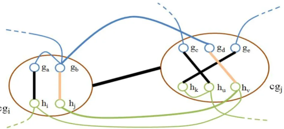
, ∈ ( ) and indicates the best permutation among all in ( ), we first look into the edge existence in (i.e. protein interaction) between and nodes. If our algorithm comes across such an edge, then the same action is performed for ℎ and ℎ nodes with . When both conditions are satisfied, the permutation ( ) gains unit edge score (Figure 2.5). When all match combinations are examined, the accumulated edge score is divided by 2 and then it is added to ( ( ) ). The total score of any permutation can be universally formulated by the equation below in any iteration :

( ( ) ) = ( ( ) ) + Λ[ ( ( ( ))) , ( ( ( ))) ] ×

2

∀ ∈ ( )

(2.1)

In equation (2.1), Λ[−, −] indicates the availability of conserved interaction between the matches of those corresponding cluster permutations, given a value of 0 or 1 and is multiplied by . There is an important reason for dividing the unit score

24

by 2. This is because we expect , when it becomes the currently investigated cluster by MP-CNet and where is the neighbor of at the time, formally ∈ ( ), to exhibit the similar satisfaction exactly between the matches ( ) of its such permutation and ( ) of the permutation of its neighbor, those which provided conserved interaction already. In this way, they mutually supplement each other by guaranteeing there really exists a conserved interaction with these selected permutations and matches. The only concern might be that if the permutation in ( ) which carries out the same interaction(s) with the one in ( ) is not the best, at the time is being investigated for edge conservation while becomes its neighbor, there is a situation that another permutation from ( ) with the convenient match can compensate this affair.

Figure 2.5 An example of external conserved interaction between clusters. Here, ( , ) match of ( ) and ( , ) match of ( ) supply a conservation externally.

After the calculation of edge scores of all permutations ∀ , we look for the best scorings to be included in ℬ′ along with the highest score achieved for . That means every permutation score ( ( ) ) are compared, just like the previous sections involving the selection of the bests. For those having more than one cluster accomplishing the same highest scores, these are broken randomly by selecting one of them and we put it into ℬ′ and, meanwhile, the highest score is

25

accumulated in another variable, denoted with Θ , hence the total best scores of all clusters are acquired in every iteration. This can be formed with the formulation in the equation below.

Θ = max ( ( ) ) , ∀

∈

(2.2)

Note that every best score from clusters summed to Θ may or may not contain the fixed scores as only we check the value of permutation scores. When a higher Θ is achieved in iteration than previously, the value is kept in maxΘ , so the highest possible score is determined until either convergence or is reached.

It should be pointed out that we do not remove ℬ of the current iteration yet. As every best permutations of all clusters is placed into ℬ′, now these values are used together to know the state of convergence of the cluster network. This is an important property that determines the continuity of conserved interaction searching, and it is checked in every iteration when all clusters are traversed for edge scores. This process is basically done by comparing the eqaulity of the best permutations of each cluster such that if every value in ℬ is completely the same

with ℬ′, for instance, ( ) = ( ), ( ) = ′( ), and so on, then

MP-CNet no longer proceeds the computation of edge scores i.e. convergence is achieved and the alignment is prepared for the output. Otherwise, it continues the computation till is reached, and ℬ ← ℬ′ is performed at the end of every iteration.

We also take another action, particularly when edge score calculation is finished thus the best permutations ( ℬ′) are decided, which could be a heuristic approach to create an alternative alignment at the end. For this purpose, ℬ is created at the beginning of the message-passing, holding how many times a

26

permutation is chosen as the best and the value corresponding to that permutation of is increased by 1 and stored in ( ) ⊂ ℬ . Note that the size of ( ) is equal to the number of permutations generated for cluster . It is implemented in every iteration till the convergence is achieved or is reached. Then, the most selected permutations among all ongoing iterations are picked up and placed in ∆ ℬ . Then, the alternative alignment is made available to the output, which can be supportive to the regular one in terms of number of conserved interactions with slightly different results. It is noted that the convergence check is not performed with ∆ ℬ; only ℬ is required for this objective.

The last portion of the message-passing of our algorithm is to present the alignment output, additionally how many conserved interactions occurred across all available matches of , and which pairs of matches provide these interactions by showing their relative nodes from and . Every 'valid' matches are gathered from clusters (i.e. not including matches involving a dummy node), hence denote ℳ to contain all these matches together. Every combination of ℳ [ ]~ℳ [ ] (1 ≤ <

, < ≤ ) is examined. Similar to what we have done previously, the matched nodes of and are taken for the existence of interactions (edges) between them in and , respectively. Those pair of matches are made available to the output and placed to ℐ when conditions are met. Then, the same process is applied to the alternative alignment by getting the valid matches and checking the presence of these (to ℐ∆ ). As a result, we create not only one steady alignment but

also a different one with our alternative intuition. We expect the number of recognized conserved interactions and those derived from matches should be identical.

27 2.5.3. Detailed Analysis and Claims

When MP-CNet achieves convergence of the input or is reached, total score, alignment, and conserved inteactions actualized by the pair of matches are presented. However, it is challenging make sure if the alignment is really optimal. About networks which are not large and too dense, relating to PPI networks and clusters, it may be somewhat predictable. During our research, we had come up with some remarkable claims that is visible to the most of the input whereas there is still extreme situations that are excluded from them. In this subsection, we would like to explain these by general basic samples, then moving to more complex ones.

The smallest cluster network we are able to reduce at most is only two cluster nodes, call and , along with only one edge available in and , connected between these clusters respectively and no edge internally. The number of subset of nodes from and in clusters can be at least one, but for comfortable analysis, let have and have subset of nodes, no matter if there exists dummy nodes. For any iteration , ℬ was already made ready in the previous iteration, − 1. As we traverse each cluster node, and so initially for , there is only one neighbor available, say ( ) = { } . Then, is set to contain matches for its best permutation, obtained from ℬ. It is noticable in this simple example that there should exist a match from ( ( ( ))) that connects the nodes and ℎ that already have an edge in and , going to other appropriate node in cluster . Likewise, should have a match between and ℎ , for some permutations. To know which of them satisfies, all matches of each permutation of are examined to check for existence, as their matches are taken one by one against the matches of the best permutation of . Suppose ( ( ( ))) is selected and these matches between two clusters achieve an external conserved

28

interaction, if the matched nodes of - and ℎ -ℎ are the edges themselves in and . In this manner, permutation ( ) gets a score by the value of /2. However, as we continue examining the permutations, there could be another one,

( ) , that has the same match, making connection between the same nodes and ℎ , thus gaining /2 score. Here, we assert that by fixing the match of such permutation of , and there are − 1 other matches remaining, maximum of ( − 1)! different forms of matches can be attained. This constitutes a significant claim such that for any cluster, ( − 1)! different permutations gain edge score by /2 if there goes one interaction from and to its neighbor cluster in ( ), for ≥ 31_{. Likewise, all of these explanations are valid for , as its neighbor}

becomes , where the matches are necessarily set for the best permutation. Here, ( − 1)! permutations can get /2, so obviously more than one of them reach the same achievement of having the best score. After these two cluster node traverses are made, however, there are ( − 1)! and ( − 1)! choices of best permutations of respective clusters that MP-CNet should select. As discussed in Section 2.5.2, a greedy approach is implemented to represent the permutations to become the best for the next iteration by first assigning to ℬ′. When no convergence is materialized then these are overwritten to ℬ, so these actions are taken again. On the other hand, due to the design of the algorithm, when there are no more iterations for message-passing by reaching , the alignment output is represented optimally. Meanwhile, here comes the better understanding of why edge score is divided by 2. As the best permutations of and together generate the same external conservation even

1

Here, (3-1)! = 2! = 2, so there is not only one permutation getting the edge score by having the same matches; also always valid for much higher number of pairs of nodes in clusters. For others, like one or two node pairs, 1! = 2! = 1 permutation can obtain the score.

29

though asynchronously, summing these scores guarantee a such external conservation truly exists.

Now, we extend this situation by inserting new edges to (or ) that goes from one cluster to another while the other remains at one edge. It should be approached with two main types: Whether these edges are connected with the other one or disconnected to observe the effects to the whole cluster network, external conservation finding and convergence. First, assume it sustains the connectivity with the existed edge. "Connectivity", hereby, means there is a common node between them, for instance, considering an edge - and the new edge - both source and target nodes are covered in different clusters, the common node provides the connectivity of these two edges. We also agree that a single edge between clusters is a connection, too. Imagine the current cluster network like this, two different nodes of in have one plausible edge and one node of from have two plausible edges while the other graph remains unaffected. Here, still possesses the probability for ( − 1)! permutations to get /2 because there is only one node (as well as match) in that can give the conserved interaction externally. If we take a look at the possibilities for , then the number of permutations that are able to obtain edge score become 2 × ( − 1)! as there are now two-to-one possible such matches for some permutations in satisfying connections between nodes with available edges in their networks. Therefore, at the end of iteration , MP-CNet now has 2 × ( − 1)! and ( − 1)! permutations to select as their bests for the next one, respectively. Total edge score, however, is still the same. We claim from this current sample that the number of available edges from one graph, travelling through two clusters and maintaining the other with one edge merely allows a cluster the possibility for up to × ( − 1)! = ! permutations have edge score, but because of

30

one edge existence of the other PPI-network graph, there is no way to multiply the total score of these two connected clusters as only one match of their such permutations can perform it. The convergence and optimal alignment is still achieved by the algorithm, but due to the increased number of permutation choices, this also raises the finite number of iterations to make it happen. Considering the edge disconnection of edges of and/or , we have conjectured that this, unfortunately, often causes no convergence for no matter how is as much as high. This is such a bizarre condition that by examining the possible best permutations ( ) for each cluster in every iteration until the maximum, the best of one or more are completely different than the previous iteration that leave MP-CNet no opportunity to make convergence, though the highest total score can be reached. The discrepancy of dissimilar best permutations of clusters repeat in at least two-iteration cycles, and by checking ℬ at , these permutation indexes cannot form the optimal alignment but partially i.e. an approximate one is encountered.

A little more complex structure between these two clusters could be that both and contain more than one edge and still going from to . This affects some permutations that achieve conserved interactions externally with more than one matches. Suppose the edges in their respective PPI-network graphs remain the connectivity for having convergence and alignment optimally, now such a permutation from ( ) possesses a likelihood that its matches against the ones of the best permutation of the neighbor clusters together produce × ( /2) edge scores, where can take any value, indicating the times of happenings of conservation with these permutation matches, here > 1 is preferred for this purpose (Figure 2.6). There can be other permutations that have edge scores but not higher than the bests when all are investigated. Therefore, this shape of two clusters

31

allow MP-CNet to make the best permutation selection of each cluster with fewer options for determining ℬ for the next iteration and can help convergence occurence by a bit less iteration made. Additionally, another important claim is obtained, thanks to our analysis, that the edge score of a cluster permutation can get at most is × ( /2). In other words, the maximum edge score of a permutation is dependent on the number of edges between two clusters whichever is lower. If there are three edges from and two edges from , going from one cluster to another, for example, then a permutation cluster edge score can be up to 2 × ( /2).

Figure 2.6 Alignment optimality between two clusters with multiple edges

The more complicated cluster network input for the algorithm is surely enough multiple clusters as real examples should contain hundreds of clusters, along with lots of possible cluster edges in terms of the clustering algorithm output. For making necessary interpretations of this form, consider simple consists of (i) three clusters where is connected to , and is connected to , (ii) four clusters where the connections are made between - and - , so two separate sub-cluster networks and, of course, edge connectivity of proteins is still maintained for

32

those. About (i), the algorithm always starts at with ( ) = { } and definitely, all permutations in ( ) are compared with the best permutation ( ) , hence there will be best-scoring permutations to choose from and similarly for , ( ) = { }. For , however, there are more neighbors detected, say ( ) = { , } and ( ) > 1. MP-CNet traverses these neighbors one by one for permutations to make external conservations with the bests of its neighbors. Here, more important matter is the maximal edge score of a permutation of a cluster being examined can go up to ( + ) × ( /2), where and denote the highest times of conservation occurences from neighbor clusters and reflect the lesser number of edges of or moving from this cluster to the related neighbor. From this vision, it is discernable for a cluster that having many neighbor connections can also bring more scores to its permutations and it will become easier for MP-CNet to select the best one if the matches of the permutation are capable of performing the most conserved interactions with the neighbor bests externally, so contributing to convergence of in a way that it can always become the best one through iterations. About (ii), the investigation of sub-network clusters are applied independently from each other such that only the neighbors can affect the others with regard to conserved interactions and determination of best permutations. On the one hand, a sub-cluster network has no influence to other familiar structure, even if the convergence happens between these clusters at iteration , they must wait for the other in order to cary out a full convergence, otherwise they are continued for searching. That is because our algorithm is designed for globally aligning the clusters (and not for local search) that all best permutations must be exactly the same with the previous selections, as indicated in Section 2.5.2 like ℬ = ℬ′. This points out a

33

disadvantage that causes more iterations to be done overall. Despite under this setting, the optimal alignment is still returned.

So far, we have elucidated a lot for necessities of alignment optimality of the cluster network by also adapting to the methods of MP-CNet. To sum the things up, we propose both and must have sustainable connectivity between each connected clusters in order to converge at a finite number of iterations and at that point the best possible alignment is made to the output, particularly achievable for small or medium sized graphs, otherwise the algorithm is progressed until for the best approximate one. Edge disconnections of protein networks across some or many clusters can cause the impossibility of convergence at all, and again an approximate alignment. In addition, we never discussed the situation of the inclusion of fixed scores (internal conserved interactions) for clusters. Here, our researches on many different structures showed that by testing the same instances with fixed scores (ℱ ) do not make any changes to the general optimality of alignment and convergence. There is a relationship between and unit scores that we always recommend the scoring schema of ≥ . This is another criterion for getting optimal alignments. Initially, permutations with best fixed scores and with the maximum plausible edge counts become the best of their related clusters before message-passing begins and have more probability to remain it for the most iterations unless another permutation has higher score. In this way, we do not see a loss of total conserved interactions that prevents the optimality but other distinct variants may be encountered like some external conservations are not presented at the end. In contrast where < , the algorithm sometimes returns less total score and significantly decreases the likelihood of the alignment to become optimal. This is not the desired situation as keeping both values equal is most convenient way. We

34

adopt the value of 1.0 for the experiments in Section 3 to see the exact number of total conserved interactions. All in all, these further explanations were made for MP-CNet to show how it works at a smooth rate of performance against the given input. 2.5.4. Discussions for Convergence

Convergence of is a crucial feature for MP-CNet as it makes the decision of if we should go on computing the edge scores of all clusters with the updated best permutations or stop immediately and progress to prepare the alignment. Here, convergence, on one hand, ensures no more conserved interactions (i.e. no higher scores) can be produced by the algorithm and also states that continuing after this point causes loss of time. When this is materialized, we always inquire the output alignment and our algorithm with these questions: (a) Does the algorithm always converge? (b) If it converges, does the alignment become optimum? (c) What is the maximum number of iterations until convergence is achieved?

Depending on the structure of both PPI networks and the cluster network which is made in the data processing stage, it is hard to come up with common and proper answers for these questions, due to the spantaneousness of constrained GNA problem and the design of our algorithm to this. Assuming simple and sparse kinds of these networks each, then the questions of our inquiry can be answered without not much difficulties. On the other hand, the matters are getting to impossibility for more complicated structures of both PPI and cluster networks. Despite the hardness, here we attempt to give general responses to these questions and mostly attribute to the claims and analysis that have been obtained during the research and development of MP-CNet, together with the results that have been encountered by many different inputs as they were explained in the previous section.