Piecewise smooth signal denoising via principal curve projections

PIECEWISE SMOOTH SIGNAL DENOISING VIA PRINCIPAL CURVE PROJECTIONS

Umut Ozertem*, Deniz Erdogmus

t,

Orhan Arikan

*

*Yahoo! Inc. Santa Clara CA, 95054,

tCSEE Dept. Oregon Health and Science University, Portland OR, 973.29

*Dept. of Electrical and Electronics Engineering, Bilkent University, TR-06800 BIlkent, Ankara

ABSTRACT

One common problem in signal denoising is that if the sig-nal has a blocky, in other words a piecewise-smooth struc-ture, the denoised signal may suffer from oversmoothed dis-continuities or exhibit artifacts very similar to Gibbs phe-nomenon. In the literature, total variation methods and some modifications on the signal reconstructions based on wavelet coefficients are proposed to overcome these problems. We take a novel approach by introducing principal curve pro-jections as an artifact-free signal denoising filter alternative. The proposed approach leads to a nonparametric denoising algorithm that does not lead to Gibbs effect or so-called

staircase type unnatural artifacts in the denoised signal.

1. INTRODUCTION

Following the additive noise model, signal denoising prob-lem can be defined as extracting themeaningful part of the

data from the observed signal by subtracting or suppress-ing noise. Although in most of the scenarios this intuitively refers to reconstruction of the original signal from the ob-served signal that is contaminated with noise; in general, the vagueness ofmeaningful part in the problem definition

here is indeed intended depending on what the problem spe-cific meaningful information is.

Under the known noise model assumption, optimal fil-tering in frequency domain is a well established topic [1]. Frequency domain filtering is conceptually simple, easily analyzable, and computationally very inexpensive. How-ever, the main drawback of this approach is obvious if the signal and the noise are not separable in the frequency do-main. Practically, in frequency domain filtering one should compromise the discontinuities in the signal, since they will be smoothed along with the noise.

As well as traditional frequency domain filtering tech-niques, current signal denoising techniques include wavelet transfonn and total variation based noise removal algorithms. These techniques stem from the idea of preserving the high

This work is partially supported by NSF ECS-0524835, and NSF-ECS0622239.

frequency components, namely discontinuities, of the sig-nal while suppressing noise. Since piecewise smooth sigsig-nal structure is typical in visual images, total variation based noise removal is first introduced in image denoising [2, 3]. Later, Vogel proposed a fixed-point iterative scheme to solve the total variation penalized least squares problem [4].

Another way to achieve discontinuity preserving denois-ing is to utilize discrete wavelet transfonn as an orthogonal basis decomposition. This method is based on decompos-ing the signal into orthogonal wavelet basis, perfonn either soft or hard thresholding to wavelet coefficients, and trans-fonn the data to the time/spatial domain by inverse discrete wavelet transfonn. Note that any orthogonal decomposi-tion of the signal can be used similarly for denoising. In such techniques the perfonnance of the denoising is typi-cally measured by the rate of decay of the basis coefficients sorted in the magnitude. In the context ofpiecewise smooth signal denoising, wavelet decomposition is known to be su-perior to other widely used choices like Fourier and co-sine decompositions [5]. Earlier techniques based on hard thresholding of the wavelet coefficients suffer from Gibbs effect like artifacts around the discontinuities. This draw-back is handled by soft thresholding of this wavelet coeffi-cients [6], and later by applying previously mentioned total variation based approaches in wavelet domain analysis [7].

Principal curves are definedby Hastie and Stuetzle [8] as"self-consistent finite length smooth curves passing from the middle of data." The literature on principal curves is

dense in algorithm design, but there is not much work on the theoretical side. We recently proposed another definition for principal curves, which describes the principal curve in tenns of the gradient and the Hessian of the data probabil-ity densprobabil-ity [9, 10] that yields constrained maximum like-lihood type algorithms. This definition stems from a dif-ferential geometric approach. In this paper, we utilize our recently proposed principal curve projections to implement a data-driven nonparametric nonlinear filter for artifact-free piecewise continuous signal denoising. The resulting fil-ter is based on the kernel density estimate (KDE) of the data, where parametric variants are possible and conceptu-ally very similar.

2. PRINCIPAL CURVES

We define the principal curve as follows: "a point in the

data feature space is on the principal curveifand onlyifthe gradient ofthe pdfis parallel to one ofthe eigenvectors of the Hessian and the remaining eigenvectors have negative eigenvalues"[9, 10]. In other words, the principal curve is essentially the ridge of the pdf.

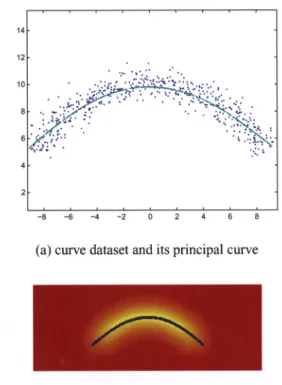
Although the details of the principal curve derivation is omitted due to restricted space, we start with a simple il-lustration of the concept here to motivate our proposition. Consider the simple illustration in Figure 1. To find the principal curve, we start with the density estimate of the data. Figure 1a shows the dataset (blue) along with the prin-cipal curve projections of all data samples (green). This is exactly where the gradient of the pdf is parallel with one of the eigenvectors ofthe Hessian of the pdf. More intuitively, the principal curve can also be thought as the ridge of the pdf. Underlying probability density along with the same principal curve is presented in Figure 1b, again for the same dataset.

Defining the principal curve in terms of the data pdf al-lows us to leave all regularization constraints to the density estimation step. This idea, in fact, is central to our approach of connecting the known problems in the principal curve fitting research to well-studied results in the density estima-tion literature. In the next secestima-tion, as we present our imple-mentation, we will present brief examples of these natural connections in the context of kernel density estimation.

14

12

-8 -6 -4 -2

(a) curve dataset and its principal curve

(b) KDE of the curve dataset and with the principal curve Fig.1.A simple illustration of the principal curve concept

3. PIECEWISE SMOOTH SIGNAL DENOISING VIA PRINCIPAL CURVE PROJECTIONS

whereti denote the sampling times. At this point, we as-sume that the original signal

s(t)

is sampled at least at the Nyquist frequency. Sampling and reconstruction are well established topics in signal processing, the details of which will are out ofthe scope ofthis paper. Also note that, as long as it preserves a blockwise continuous nature, the rest ofthe paper does not depend on how x is constructed. Using time This section will present the details of the proposed prin-cipal curve denoising filter, as well as the selection of the kernel bandwidth, which is a critical step in the implementa-tion. To utilize principal curve projections, one should start with translating the signal into a suitable feature space. The most intuitive selection is to use the samples of the noisy signal itself along with the associated time indices. Assum-ing that the observed signalx(

t)

is the original signal buried in additive noise that is,

x(t)

=

s(t)

+

n(t),

this yields

(2)

N

p(x)

=

L

K~i

(x - Xi)

i=l

delayed versions of the observed signal or any other repre-sentation of it based on orthogonal decompositions can also be used. For now, we leave this further investigation as fu-ture work and focus on the simple feafu-ture construct given in (1).

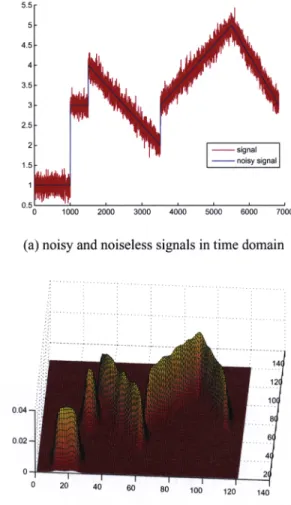
Figure 2 depicts an illustrative piecewise smooth signal with its noisy version as well as the kernel density estimate of the noisy signal. Now consider the kernel density esti-mate of the noisy signal which is given by

where~idenotes the covariance of the kernel function for theith _{sample}. Note that the density estimate of x in the}

vicinity of discontinuities is not effected much by the sam-ples on the opposite side of the discontinuity. Although these are close -or maybe even subsequent- samples along the time axis, the discontinuity in signal value makes them sufficiently distant in the x space. For unimodal additive noise distributions (as in the case ofadditive Gaussian noise)

IThis density estimate is given for the most general case of data-dependent variable bandwidth KDE. For fixed bandwidth version, one can just drop this data dependency.

(1)

. _ [x(t

i ) ]

5.5

4.5

3.5

2.5

1000 2000 3000 4000 5000 6000 7000

(a) noisy and noiseless signals in time domain

0.04

0.02

M 100 1~ 1~

(b) KDE of the noisy signal in x space

Fig. 2. The underlying noiseless signal and its noisy coun-terpart

the noiseless signal will most likely be a smoother signal

passing through the middleof the observed noisy samples. Hence, principal curve naturally fits into the context of arti-fact free signal denoising of piecewise smooth signals.

As we proposed in earlier publications [9, 10], principal curve projection can be achieved by a likelihood maximiza-tion in a constrained space, and our earlier proposed algo-rithms can directly be used to identify the principal curve. However, particularly for this denoising application, we have a much easier scenario due to the following:

1. Only the samples of the principal curve at time in-dices

tl

< ... <

tNare sufficient. Higher time reso-lution or seeking for the portion ofthe principal curve that lies outside the given time interval is unnecessary. 2. Unlike the general case of random vectors, the sec-ond dimension, which represents the time indices of

signal samples is deterministic; in the case ofuniform sampling, we can model this density as being uniform for theoretical analysis.

One can select the initialization ofthe algorithm and the constrained space of the projection using these two simplifi-cations. At this point, starting from the data samples them-selves, and selecting the constrained space as thet

=

tifor each data sample is our choice for the two following rea-sons, under the assumption of a unimodal zero mean noise density:

1. Selecting constrained space orthogonal to time index guarantees that there is only one denoised signal value at all time indices.

2. One important observation here is that at the peak of the pdf in each constrained spacet

=

ti is very close to principal curve.

With the above selections of the initialization and the constrained space, the principal curve projection turns out to be as simple as evaluating the mean shift update and pro-jecting it onto the first dimension - the vertical axis in Figure 2a. Although it is close, the optimizer ofthe algorithm is not on the principal curve. Therefore, we use the SCMS algo-rithm [10] to project these points onto the principal curve, and assign the signal values as the denoised signal by keep-ing the time indices the same. We skip the derivation of SCMS here, yet we still provide the details of implementa-tion in Table 1, steps 5-10.

Mean shift is a very commonly used iterative procedure that maps the data points to the corresponding peak of the probability density, where the gradient is equal to zero and all eigenvalues of the Hessian are non-positive [11]. Partic-ularly for a Gaussian kernel function with fixed bandwidth, taking the derivative of (2) with respect to x, and equating it to zero, one obtains

p(X)

=

~~l G~i (x -

Xi)

X

~~l ~il G~i (x -

Xi) -

~i:l

Xi

~il Ga(x -

Xi)

=

0

(3) Reorganizing terms and solving for x yields the well-known mean shift update [11]

N N

X~

m(x)

=

(L

EilG~i(X-Xi))-l

L

EilG~i(X-Xi)Xi

i=l i=l

(4) Finally, to achieve the desired projection, at each iteration the update in the second dimension has to be removed. This projection has a time complexity of

O(N)

per sample per iteration. Table1briefly presents the overall algorithm.

(a) (b) (c) (d)

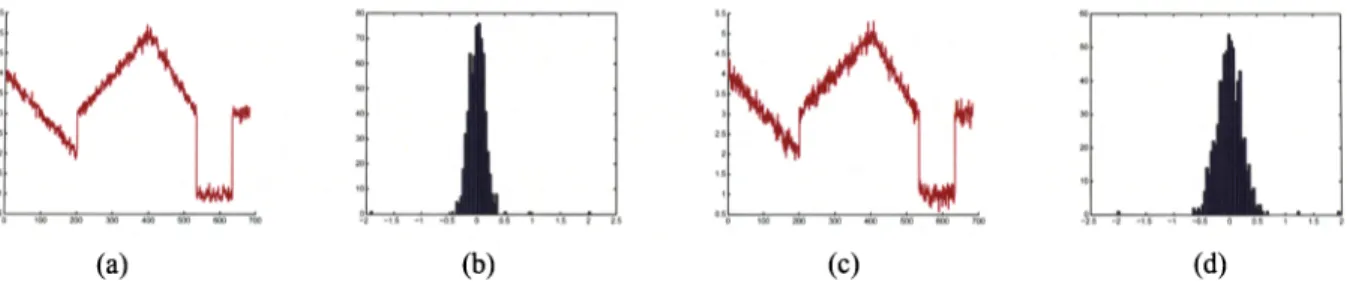
Fig.

3. Two realizations of the same piecewise smooth signal for two different SNR levels are shown in (a) and (b), along with their time difference histograms in (c) and (d).

3.1. Selection of the Kernel Bandwidth

Table1. Principal curve signal denoising

1. Build the feature space x, select the kernel bandwidth

aof the Gaussian kernel.

2. Evaluate the mean shift update using (4).

3. Project the mean shift update to

[6]'

so that the mean shift procedure remains in the constrained space.

4. If convergence not achieved, go to step 2, if conver-gence is achieved go to the next step.

5. For every trajectory evaluate the mean shift update in (4).

6. Evaluate the gradient, the Hessian, and perform the eigendecompositionofE-1_(x(k))

₌

vrv.

7. Let v be the leading eigenvector of~-1 .

8. i=vvTm(x(k))

9. If

IgTHgl/llgllllHgll

>

threshold then slop, else x(k

+

1)

f -

i.

10. If convergence is not achieved, incrementkand go to step 6.

Selecting the bandwidth of the Gaussian kernel is a very important step in the implementation that severely affects the performance of the algorithm. Fortunately, literature on density estimation is rich on how to select the kernel width, and methods in the literature extend from simple heuristics to more technically sound approaches like maximum likeli-hood [12, 13, 14, 15, 16].

All above mentioned techniques are general purpose ker-nel bandwidth selection methods that blindly approach the data. Particularly for this problem, one can also select the kernel bandwidth by considering the actual physical mean-ing of the data. If the amount of noise and the amount of fluctuations at the discontinuities are at different scales, ker-nel bandwidth selection can be achieved by observing prob-ability density of the time difference of the signal. Figure 3presents two realizations of a piecewise smooth signal at different noise levels. Although this may not be the general case for all noise levels, note that the noise distribution and discontinuities are clearly identifiable in this difference his-togram for the presented signals, where the difference val-ues at the discontinuities seem like outliers of the Gaussian noise distribution.

4. EXPERIMENTAL RESULTS

This section presents the performance of the proposed de-noising algorithm. To be able to control the SNR level in the experiments, synthetic examples are used, and denoising performance is reported for different SNR values. Another important point is, of course, the performance around the discontinuities. As well as quantitative results, we present the actual signal plots to provide a visual comparison of the noisy and denoised signals at different SNR levels. At the discontinuities, principal curve denoising does not yield any pseudo-Gibbs artifact effects like discrete wavelet denois-ing techniques, or any oversmoothdenois-ing like frequency do-main filtering. As one can observe from the denoising on the ramp-signal components, principal curve denoising also

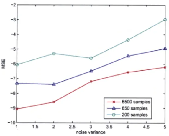
Fig. 4. MSE between the noiseless signal and output of the denoising filter for different SNR levels

does not yield any staircase type effects like total variation based methods.

Figure 4 presents the denoising results for the noiseless signal presented in Figure 2 (blue) for different SNR lev-els. We measure the performance MSE between the output of principal curve denoising and the underlying noiseless signal. Here we also compare the number of samples used in the principal curve estimation. The principal curve pro-jection depends on the accuracy of the underlying density estimate. As the statistical variance of the density estimate increases in low sampling rates, and the performance of the principal curve denoising decreases.

For the same signals ofdifferent SNR and sampling rates, which are compared in Figure 4, Figure 5 presents the noisy and denoised time signal pairs. For all above experiments, we use the maximum likelihood kernel size for each signal. So, we learn the kernel bandwidth from the signal directly, and use a different kernel bandwidth for each realization of the signal. Maximum likelihood training automatically adapts the kernel bandwidth according to the noise level of the data, and evaluating the maximum likelihood ker-nel bandwidth is a well-known topic and details are omitted here [12].

As a final remark, note that we are not presenting any comparisons with the other principal curve approaches in the literature. Since, by definition, they are looking for smooth curves, earlier principal curve algorithms are not suitable for piecewise smooth signals, and oversmoothing on the discontinuities would be unavoidable.

6. REFERENCES

denoising filter can successfully preserve the sharp discon-tinuities in the data under the additive unimodal noise as-sumption, without introducing any smoothing, high frequency Gibbs effect like artifacts or staircase type effects.

The proposed scheme allows one to translate common problems in piecewise smooth signal denoising into selec-tion of the kernel funcselec-tion. For example, as opposed to ear-lier methods in the piecewise-smooth signal denoising that are based on total variation or discrete wavelet transform, principal curve based denoising is much easier to build an online counterpart just by selecting a finite support kernel function. For a KDE built using a kernel function of online support, the subset of signal samples that affect the pdf on a particular point of interest are clearly given, yielding an online version of the algorithm directly. Adapting the prin-cipal curve denoising for nonstationary or data-dependent noise distributions is also straightfolWard. With the current implementation, it is computationally more expensive than earlier methods in the literature. At this point, KDE with finite support kernel will save a lot of computational effort, which can bring the computational cost up to linear time complexity. All these are left as future prospects to investi-gate.

[6] David L. Donoho, "De-noising by soft-thresholding,"

IEEE Transactions on Information Theory,vol. 41, no. 3,pp.613-627, 1995.

[4] C.R.Vogel andM. E. Oman, "Iterative methods for total variation denoising,"SIAM Journal on Scientific Computing,vol. 17, no. 1, pp. 227-238,1996. [5] Albert Cohen and Jean-Pierre D'Ales, "Nonlinear

ap-proximation of random functions," SIAM Journal on

Applied Mathematics, vol. 57, no. 2, pp. 518-540,

1997.

[2] Leonid I. Rudin, Stanley Osher, and Emad Fatemi, "Nonlinear total variation based noise removal algo-rithms," Phys. D,vol. 60, no. 1-4, pp. 259-268, 1992. [3] David C. Dobson and Fadil Santosa, "Recovery of

blocky images from noisy and blurred data," SIAM Journal on Applied Mathematics, vol. 56, no. 4, pp. 1181-1198, 1996.

[1] Simon Haykin, Adaptive filter theory (3rd ed.), Prentice-Hall, Inc., Upper Saddle River, NJ, USA, 1996. 4.5 3.5 noise variance 2.5 -2 -3 -4 -5 w en -::; -7 -8 -9 -10 1 1.5 5. CONCLUSIONS

In this paper, we propose to use principal curves for artifact-free denoising of piecewise smooth signals. The proposed

[7] Sylvain Durand and Jacques Froment, "Reconstruc-tion of wavelet coefficients using total varia"Reconstruc-tion min-imization," SIAMJ. Sci. Comput., vol. 24, no. 5, pp. 1754-1767,2002.

(a) (f) (b) (g) (c) (h) (d) (i) (e) (j) (k) (I) (m) (n) (0)

Fig. 5. Two realizations of the same piecewise smooth signal for two different SNR levels are shown in (a) and (b), along with their time difference histograms in (c) and (d).

[8] T. Hastie and W. Stuetzle, "Principal curves," Jour. Am. Statistical Assoc., vol. 84, pp. 502-516, 1989.

[9] Deniz Erdogmus and Umut Ozertem, "Self-consistent locally defined principal surfaces," inProceedings of International Conference on Acoustics, Speech, and Signal Processing, 2007, pp. 11549-11552.

[10] Dmut Ozertem and Deniz Erdogmus, "Local condi-tions for critical and principal manifolds," in Pro-ceedings of International Conference on Acoustics, Speech, and Signal Processing, 2008.

[11] Y. Cheng, "Mean shift, mode seeking, and clustering,"

IEEE Trans. on Pattern Analysis and Machine Intelli-gence, vol. 17, no. 8,pp. 790-799,1995.

[12] Richard

o.

Duda, Peter E. Hart, and David G. Stork, Pattern Classification (2nd Edition),

Wiley-Interscience, November 2000.

[13] B. W. Silverman,Density Estimationfor Statistics and Data Analysis, Chapman& Hall/CRC, April 1986.

[14] Emanuel Parzen, "On estimation of a probability den-sity function and mode," The Annals ofMathematical Statistics, vol. 33,no.3,pp. 1065-1076,1962.

[15] Dorin Comaniciu, "An algorithm for data-driven bandwidth selection," IEEE Trans. Pattern Anal. Mach. Intell., vol. 25, no. 2, pp. 281-288, 2003. [16] Lihi Zelnik-Manor and Pietro Perona, "Self-tuning