Başlık: Primary production estimation of Çankırı province’s rangelands using light use efficiency (LUE) model with satellite data and agrometshell moduleYazar(lar):ÜNAL, Ediz; BAYRAMİN, İlhamiCilt: 22 Sayı: 4 Sayfa: 555-565 DOI: 10.1501/Tarimbil_000000141

(1)

Dergi web sayfası:

www.agri.ankara.edu.tr/dergi www.agri.ankara.edu.tr/journalJournal homepage:

TARIM BİLİMLERİ DERGİSİ

—

JOURNAL OF AGRICUL

TURAL SCIENCES

22 (2016) 555-565

Primary Production Estimation of Çankırı Province’s Rangelands

Using Light Use Efficiency (LUE) Model with Satellite Data and

AgrometShell Module

Ediz ÜNALa_{, İlhami BAYRAMİN}b

a_{Field Crops Central Research Institute, Şehit Cem Ersever Street, No: 9-11, Ankara, TURKEY}

b_{Ankara University, Faculty of Agriculture, Department of Soil Science and Plant Nutrition, 06110, Ankara, TURKEY} ARTICLE INFO

Research Article

Corresponding Author: Ediz ÜNAL, E-mail: eunal@tagem.gov.tr, Tel: +90 (312) 343 10 50 Received: 25 February 2014, Received in Revised Form: 14 August 2015, Accepted: 14 August 2015

ABSTRACT

In this study, monthly and annual gross primary production (GPP) of rangelands in Çankırı province for the period of 2000-2009 was calculated using light use efficiency (LUE) model with the inputs of satellite data and AgrometShell module. The average production of rangelands varied seasonally and annually (from 12630 to 37701 tons) and was approximately 17800 tons for the last ten years. The amount of rainfall and changing number of animal grazing in the region probably led to the variation. Model performance was tested with integrated normalized difference vegetation index (INDVI) approach which produced a moderate significant correlation (R2_{= 0.69, P<0.05) between LUE model} gross primary productivity (GPP) output and INDVI values. On the other hand, comparison of modelled results of annual gross primary production (GPP) with above ground measurements, indicated that correlation between the variables were insignificant (r = 0.60, P>0.05 for 2008, r= 0.41, P>0.05 for 2009) due to some factors such as sampled plant type, scale differences between satellite data and ground sample size, and subjective sampling errors. This study indicates that LUE Model together with the inputs of AgrometShell module is suitable tool for estimation of rangeland primary production. Keywords: Biomass; Çankırı; Range; Remote sensing; Vegetation

Uydu Verisi ve AgrometShell Modülü ile Işık Kullanım Etkinliği (LUE)

Modeli Kullanarak Çankırı İli Meralarının Birincil Üretim Tahmini

ESER BİLGİSİ

Araştırma Makalesi

Sorumlu Yazar: Ediz ÜNAL, E-posta: eunal@tagem.gov.tr, Tel: +90 (312) 343 10 50 Geliş Tarihi: 25 Şubat 2014, Düzeltmelerin Gelişi: 14 Ağustos 2015, Kabul: 14 Ağustos 2015

ÖZET

Bu çalışmada, Çankırı meralarının 2000-2009 arasındaki aylık ve yıllık toplam birincil üretimleri ışık kullanım etkinliği modeli ile hesaplanmıştır. Elde edilen bulgulara göre il sınırları içinde kalan meraların son on yıllık ortalama birincil üretimi yaklaşık 17877 tondur ve bu üretim hem mevsimsel hem de yıllık olarak (12630-37701 ton arası) değişkenlik

(2)

Primary Production Estimation of Çankırı Province’s Rangelands Using Light Use Efficiency (LUE) Model..., Ünal & Bayramin

556

Ta r ı m B i l i m l e r i D e r g i s i – J o u r n a l o f A g r i c u l t u r a l S c i e n c e s 22 (2016) 555-565

1. Introduction

Rangelands are important natural resources for livestock feeding and providing habitats for biological diversity. Being a challenging issue, assessing productivity and gross primary production (GPP) of rangelands is important for their efficient management. The employment of remote sensing which has been the most frequently used method utilizes two approaches; a) establishing relationships between spectral reflectance and biomass (Tucker et al 1983) and b) modelling GPP from remotely sensed spectral reflectance to estimate the amount of absorbed photosynthetically active radiation (APAR) (Brogaard et al 2004). A light use efficiency (LUE) approach is widely applied concept for modelling the GPP (Goetz et al 1999; Hilker et al 2008), and expresses the GPP as a product of the APAR. This approach is the main component of the current study based on the idea that biological production is directly proportional to the photosynthetically active radiation (PAR) absorbed by the green vegetation (Monteith 1972).

The revised model of Seaquist et al (2003) presented in Equation 1 was used in this study, because it includes environmental effects (drought, temperature, pollution, nutrient deficiency, illness etc.) as stress factors which play an important role in biological activities of the plant and hence in the GPP.

2 1. Introduction

Rangelands are important natural resources for livestock feeding and providing habitats for biological diversity. Being a challenging issue, assessing productivity and gross primary production (GPP) of rangelands is important for their efficient management. The employment of remote sensing that could be the most frequently used method utilizes two approaches; a) establishing relationships between spectral reflectance and biomass (Tucker et al 1983) and b) modelling GPP from remotely sensed spectral reflectance to estimate the amount of absorbed photosynthetically active radiation (APAR) (Brogaard et al 2004). A light use efficiency (LUE) approach is widely applied concept for modelling the GPP (Goetz et al 1999; Hilker et al 2008), and expresses the GPP as a product of the APAR. This approach is the main component of the current study based on the idea that biological production is directly proportional to the photosynthetically active radiation (PAR) absorbed by the green vegetation (Monteith 1972).

The revised model of Seaquist et al (2003) presented in Equation 1 was used in this study, because it includes environmental effects (drought, temperature, pollution, nutrient deficiency, illness etc.) as stress factors which play an important role in biological activities of the plant and hence in the GPP.

n 1

i

εp

ε

FPAR

PAR

GPP

(1)

Where; GPP, gross primary production (g m-2_{) converted to dry plant matter (DM) through}

photosynthesis; Ɛp, LUE factor (g DM MJ-2_{) expressing conversion of light energy into dry mass; Ɛ,}

unitless environmental stress factor; PAR, photosynthetic active radiation (MJ m-2_{) of sun light in the}

spectral range of 400-700 nm and FPAR, fraction of absorbed light by vegetation.

The main objective of this study was to estimate and map annual and monthly GPPs of rangelands in Çankırı province using a light use efficiency model. The following steps were also achieved by reaching the main objective; 1) a validation of calculated GPP by ground data and 2) performing a sensitivity analysis of the model variables.

2. Material and Methods

2.1. Study area

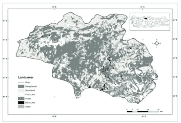
The study area is Çankırı province located in the Central Anatolia, Turkey (Figure 1). The landscape of Çankırı is mostly mountainous with hilly topography covering approximately 60% of the province. The average elevation is 723 m with hills and plateaus interrupted by Ilgaz Mountain ranges. Continental climate dominates the region with long term average rainfall of 500 mm. The land is mostly bare on the hills and plateaus, while the mountains are covered with coniferous trees. Foot lands are generally used for grain cultivation. Soil erosion is prevalent across the province, which explains why the non-cropped lands are used mostly as rangelands. These rangelands have some characteristics of desert plant species, resulting from low rainfall of 300-500 mm and over grazing (Ketenoğlu et al 1983). The botanical composition of rangelands generally consists of short grass (Festuca sp, Poa sp.), broad leaves (Medicago sp.) and various thorny species (Astragalus sp.) (Kurt et al 2006).

In this study, the GPP was calculated both monthly and annually for 10 years (2000-2009) for the active vegetation period of a growing season that starts with first leaf appearance and ends with senescence. The growing season was divided into 10-day periods (dekad) totaling to 14 dekads for each year. The first dekad starts on March 20th_{and ends on March 31}st_{. The last dekad spans from August 1}st_{to August 10}th_.

(1)

Where; GPP, gross primary production (g m-2_{) converted to dry plant matter (DM) through}

photosynthesis; Ɛp, LUE factor (g DM MJ-2₎

expressing conversion of light energy into dry mass; Ɛ, unitless environmental stress factor; PAR, photosynthetic active radiation (MJ m-2_{) of sun light}

in the spectral range of 400-700 nm and FPAR, fraction of absorbed light by vegetation.

The main objective of this study was to estimate and map annual and monthly GPPs of rangelands in Çankırı province using a light use efficiency model. The following steps were also achieved by reaching the main objective; 1) a validation of calculated GPP by ground data and 2) performing a sensitivity analysis of the model variables.

2. Material and Methods

2.1. Study area

The study area is Çankırı province located in the Central Anatolia, Turkey (Figure 1). The landscape of Çankırı is mostly mountainous with hilly topography covering approximately 60% of the province. The average elevation is 723 m with hills and plateaus interrupted by Ilgaz Mountain ranges. Continental climate dominates the region with long term average rainfall of 500 mm. The land is mostly bare on the hills and plateaus, while the mountains are covered with coniferous trees. Foot lands are generally used for grain cultivation. Soil erosion is prevalent across the province, which explains why the non-cropped lands are used mostly as rangelands.

göstermektedir. Bu değişkenliğin ana sebepleri içinde bölgeye düşen yağış miktarı ve otlayan hayvan sayısındaki değişimler gösterilebilir. Model performansı, toplanmış normalize edilmiş farklılık indeksi (INDVI) ile test edilmiştir. Test sonucuna göre, INDVI ve toplam birincil üretim arasında orta seviyede bir ilişki (R2_{= 0.69, P<0.05) bulunmuştur.} Uygulanan hassaslık analizi sonuçları, orantılı fotosentetik aktif radyasyonun (FPAR) en hassas değişken olduğunu göstermiştir. Diğer taraftan, modelden hesaplanan yıllık birincil üretim (GPP) değerleri ve arazi çalışmaları ile hesaplanan biyokütle arasında önemsiz ilişki bulunmuştur (r = 0.60, P>0.05, 2008; r= 0.41, P>0.05, 2009). Örneklenen bitki türleri, kişisel örnekleme hataları ve uydu verileri ile örnekleme alanı arasındaki ölçek farklılığı ilişki çıkmamasının ana sebepleri olarak gösterilebilir. Bu çalışma, AgrometShell girdilerini kullanan LUE modelinin meralarda birincil üretim miktarının tahmin edilmesinde iyi bir araç olduğunu ortaya koymaktadır.

Anahtar Kelimeler: Biyokütle; Çankırı; Mera; Uzaktan algılama; Vejetasyon

(3)

557

Ta r ı m B i l i m l e r i D e r g i s i – J o u r n a l o f A g r i c u l t u r a l S c i e n c e s 22 (2016) 555-565 These rangelands have some characteristics of desert

plant species, resulting from low rainfall of 300-500 mm and over grazing (Ketenoğlu et al 1983). The botanical composition of rangelands generally consists of short grass (Festuca sp, Poa sp.), broad leaves (Medicago sp.) and various thorny species (Astragalus sp.) (Kurt et al 2006).

In this study, the GPP was calculated both monthly and annually for 10 years (2000-2009) for the active vegetation period of a growing season that starts with first leaf appearance and ends with senescence. The growing season was divided into 10-day periods (dekad) totaling to 14 dekads for each year. The first dekad starts on March 20th_and

ends on March 31st_{. The last dekad spans from}

August 1st_{to August 10}th_.

Figure 1- Location of study area and land cover classes

Şekil 1- Çalışma alanı ve arazi örtüsü sınıfları

2.2. Used data

The meteorological data stored in AgrometShell module retrieved from 36 automatic weather stations (AWS) distributed over the province of Çankırı and neighboring provinces (Figure 2). The AWSs measured many weather parameters some of which were the inputs in database of AgrometShell module developed by FAO Environment and Natural Resources Service (SDRN). The module provides a toolbox for agro-meteorological crop monitoring and forecasting (Mukhala & Hoefsloot

2004) and includes a database of weather data as 10-day average of temperature (°C), solar radiation (Cal m-2_{), wind speed (m s}-1_{) and 10-day sum of}

rainfall (mm) as well as crop specific information such as crop type, crop cycle length, irrigation, etc. AgrometShell module runs a water balance model to produce actual evapotranspiration (AET) and potential evapotranspiration (PET) which were used later for water stress calculation in LUE model. Calculated PET and AET values were then converted into grid format by the inverse distance weighting (IDW) kriging interpolation method (Ha et al 2011) to generate surfaces with same cell size of 1 km of NDVI data.

Figure 2- Meteorological stations and survey points

Şekil 2- Meteoroloji istasyonları ve sörvey noktaları

NDVI images were used as satellite data, which is widely regarded as measurements of surface vegetation condition and dynamics and indicates the greenness of live vegetation (Huete et al 2002). NDVI is numerically calculated from (NIR-RED/NIR+RED). RED and NIR stand for the spectral reflectance measurements acquired in red and near-infrared regions of the spectrum, respectively. SPOT-Vegetation (SPOT-Veg) 10-days maximum value composite (MVC) NDVI images (S-10 product) were used in the model. S10 data were derived from physical products, which were surface reflectance’s corrected for molecular and aerosol scattering, water vapor, ozone and other gas absorption (Holben 1986). A total of 140 composited

(4)

558

Ta r ı m B i l i m l e r i D e r g i s i – J o u r n a l o f A g r i c u l t u r a l S c i e n c e s 22 (2016) 555-565 SPOT 10-day MVC NDVI images, hereafter called

NDVI, covering a 10 year (2000-2009) time period was obtained from ARTEMIS Project of Food and Agricultural Organization (FAO) of United Nations. The NDVI images coincided with growing season dekads.

Vector dataset (shapefile polygon) of rangeland borders produced earlier throughout the National Rangeland Project (Mermer et al 2012) was used as a mask file to exclude the areas other than rangelands for which the GPP was calculated.

Reference data were obtained from the field surveys in both July of 2008 and 2009. Stratified random sampling method was applied to determine field visit locations. 1/25000 scaled topographic map grids were used as sampling frame laid over the rangeland polygons as upper layer in a geographic information software (GIS). Automatically generated random points intersecting both rangeland polygons and map grids were selected as sampling points. The number of sampling points was determined by the approach that each map grid had at least two survey locations representing rangelands in the grid (Anonymous 2012). A total of 41 points were identified (Figure 2) for field measurements which included registering botanical composition of 1 m2_{quadrats and cutting the live}

vegetation in each quadrat. Clipped vegetation was dried at sun for 7-10 days and then weighed as a dry mass (g m-2_).

2.3. Model application

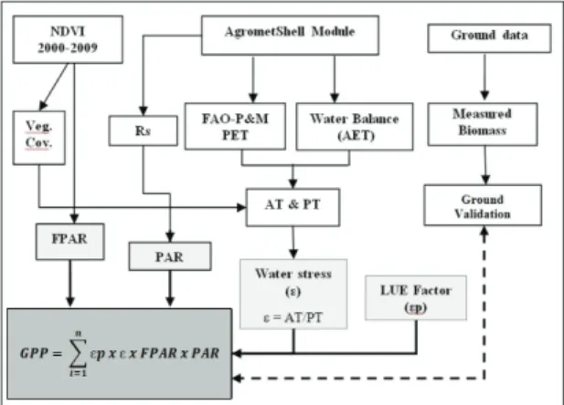
Primary production considers biomass accumulation in vegetation as the results of succession stages during which sun light energy is intercepted (Monteith 1972). Primary production is deduced as the product of radiation energy (PAR), fraction of PAR by the plant (FPAR), conversion efficiency of absorbed radiation into biomass (LUE factor) and environmental factor (stress factor). Therefore, the primary production is assumed to be proportional to these variables (Equation 1).

Methodology used similar to the one that Seaquist et al (2003) and Brogaard et al (2004) employed was

revised for potential evapotranspiration (PET) and actual evapotranspiration (AET) calculations. For the PET calculations, the FAO Penman-Monteith (Allen et al 1998) method was used, while AET was calculated by FAO AgrometShell water balance model. 10-day average PAR, FPAR and stress factors rasterized as grid format with the same spatial size of NDVI data (1 km2_{) were used in the model, while LUE}

factor was used as constant. Graphical representation of the LUE model is shown in Figure 3.

Figure 3- Graphical representation of LUE model

Şekil 3- LUE Modelinin grafiksel gösterimi

2.3.1. Photosynthetic active radiation (PAR)

PAR is a part of total incoming solar radiation in the visible spectrum (400-700 nm), which shows distinct temporal and spatial patterns due to varying atmospheric conditions (Uzun & Demir 2012). Only the PAR of total solar radiation can be used by green vegetation to produce organic matter through photosynthesis. The common and simple method to calculate the PAR is to proportionate solar radiation by total radiation received at the surface. The PAR was calculated from the solar radiation (MJ m-2₎

which was measured at meteorological station. The solar radiation incident on canopies tends to contain a relatively constant fraction of PAR varying from 45% to 50% depending on location and sky conditions (Le Roux et al 1997). On average, 48% of PAR ratio was used in calculations.

(5)

559

2.3.2. Fractioned photosynthetic active radiation (FPAR)

FPAR is the fraction of the absorbed PAR by the plant canopy and can generally be calculated by either physical models (Los et al 2005) or empirical methods (Huete et al 2002) taking into account of spectral vegetation indexes. The most known index is NDVI which relates to the FPAR given in Equation 2 (Goetz et al 1999).

NDVI b

a

FPAR= ± × (2)

Where; a and b, correlation coefficients. For the FPAR calculation, empirical method was used in this study as used by Seaquist et al (2003) and Brogaard et al (2004). The only difference was the use of additional coefficients. Background and dead materials play a substantial role on the FPAR, especially during senescence period of the plant. The FPAR absorbed by dead material reaches by 20% (Le Roux et al 1997) and thus, the FPAR value decreases gradually after development stage. We therefore added the coefficient of 0.80 to the FPAR equation to compensate dead material effects for the period of senescence which corresponds to between July 1st_{and August 10}th_{(Equation 3). During the}

initial and development stage (March 20th_-July

31st_{), no additional coefficient was added to FPAR}

equation (Equation 4).

FPAR = (1.67x(NDVI) - 0.07) x 0.80 (3)

FPAR = 1.67x(NDVI) - 0.07 (4)

2.3.3. LUE factor (ɛp)

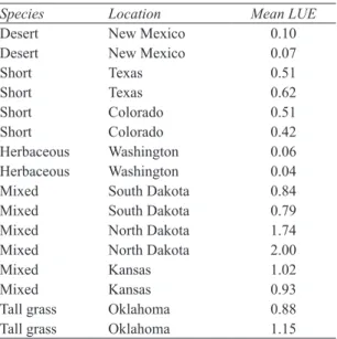
LUE factor, regarded as empirical constant, represents the actual efficiency of a absorbed radiation energy used by plants to produce biomass. Seasonal changes in LUE factor are closely related to soil water content and phenological stage of the plant (Prince 1991). In the case that available water in the soil is adequate, the value of LUE factor in early stage is higher than the one in development stage of the plant (Le Roux et al 1997). The available water is assumed to be adequate in the early stages of rangeland plants in the study area. According to Sims & Singh (1978), mean LUE values measured

for short grass species ranged between 0.42 and 0.62. Therefore a higher LUE value of 0.62 for early stage corresponding the period of March 20-May 10 was used, while the lower LUE value of 0.42 was used for the remaining stages of May 10-August 10. These values (Table 1) were used in the model, because there were not any measured LUE values for our study area where the botanical compositions consisted of mostly short grass steppe.

Table 1- Measured mean LUE values (Sims & Singh 1978)

Çizelge 1- Ölçülmüş ortalama LUE değerleri

Species Location Mean LUE

Desert New Mexico 0.10 Desert New Mexico 0.07

Short Texas 0.51 Short Texas 0.62 Short Colorado 0.51 Short Colorado 0.42 Herbaceous Washington 0.06 Herbaceous Washington 0.04 Mixed South Dakota 0.84 Mixed South Dakota 0.79 Mixed North Dakota 1.74 Mixed North Dakota 2.00 Mixed Kansas 1.02 Mixed Kansas 0.93 Tall grass Oklahoma 0.88 Tall grass Oklahoma 1.15 2.3.4. Stress factor (ɛ)

The stress component of the model is presented by lack of adequate soil moisture which plays an important role in biological activities of the plant. A stress factor was used in the LUE models as a part of a scalar environment factor (ε) in which drought, temperature, pollution, nutrient deficiency, illness and other elements were covered (Prince 1991). The stress factor was calculated by the ratio of actual transpiration (AT) to potential transpiration (PT) (Equation 5).

6

2.3.4. Stress factor (ɛ)

PT

AT ₍₅₎

Where; epsilon, ɛ, stress factor in the model; AT (mm), term emphasizes evaporated water during respiration process of plant, and PT, transpiration (mm) when there is no soil water deficit. The AT was calculated by multiplying actual evapotranspiration (AET) with fraction of vegetation cover (FVC) (Equation 6).

FVC AET

AT (6) Where; AET (actual evapotranspiration, mm), total water loss from both soil and plant during respiration. It was calculated based on the water balance model that FAO AgrometShell module performs (Mukhala & Hoefsloot 2004). The FVC was calculated from NDVI data (Equation 7).

2 s v s - NDVI NDVI I NDVI - NDV FVC (7)

Where; FVC, values range between 0 and 1 corresponding non vegetation and full vegetation cover, respectively; NDVIs, pixel value of NDVI corresponding non vegetation; NDVIv, full vegetation cover of

the NDVI and NDVI, cell-specific NDVI value in the vegetation map.

The PT is the rate of transpiration that occurs in a large area completely covered with vegetation with access to unlimited water supply and calculated by multiplying the FVC with the potential evapotranspiration (PET) and crop coefficient (Kc) (Equation 8).

FVC PET Kc

PT (8) Kc incorporates crop characteristics and effects of evaporation from the soil. A value of 0.85 was used for the development stage of vegetation, during which the Kc corresponds to amount of ground cover and plant development (Wight & Hanks 1981). For the calculation of PET, FAO’s Penman-Monteith method was used, which considers many parameters related to the evapotranspiration process such as solar radiation, air temperature, vapor pressure deficit and wind speed (Allen et al 1998). All these parameters were composited as 10-day average to coincidence with NDVI data.

3. Results and Discussion

3.1. Monthly and annual production

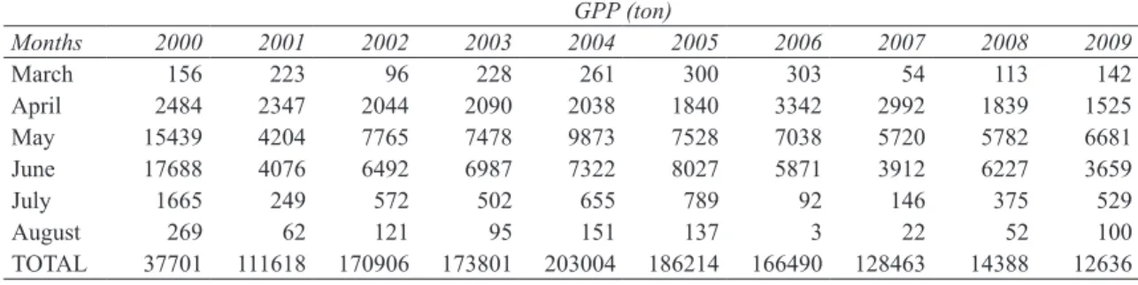
Monthly and annual primary production calculations with LUE model were presented in Table 2. The rangelands were estimated to produce 17877 tons of 10 year mean annual production in approximately 301939 hectares of range area.

(6)

560

Ta r ı m B i l i m l e r i D e r g i s i – J o u r n a l o f A g r i c u l t u r a l S c i e n c e s 22 (2016) 555-565 Where; epsilon, ɛ, stress factor in the model; AT

(mm), term emphasizes evaporated water during respiration process of plant, and PT, potential transpiration (mm) when there is no soil water deficit. The AT was calculated by multiplying actual evapotranspiration (AET) with fraction of vegetation cover (FVC) (Equation 6).

6

PT

AT ₍₅₎

FVC AET

FVC PET Kc

3. Results and Discussion

(6) Where; AET (actual evapotranspiration, mm), total water loss from both soil and plant during respiration. It was calculated based on the water balance model that FAO AgrometShell module performs (Mukhala & Hoefsloot 2004). The FVC was calculated from NDVI data (Equation 7).

6

PT

AT ₍₅₎

FVC AET

FVC PET Kc

3. Results and Discussion

(7) Where; FVC, values range between 0 and 1 corresponding non vegetation and full vegetation cover, respectively; NDVI_s, pixel value of NDVI corresponding non vegetation; NDVI_v, full vegetation cover of the NDVI and NDVI, cell-specific NDVI value in the vegetation map.

6

PT

AT ₍₅₎

FVC AET

AT (6)

Where; AET (actual evapotranspiration, mm), total water loss from both soil and plant during respiration. It was calculated based on the water balance model that FAO AgrometShell module performs (Mukhala & Hoefsloot 2004). The FVC was calculated from NDVI data (Equation 7).

FVC PET Kc

3. Results and Discussion

(8)

Kc incorporates crop characteristics and effects of evaporation from the soil. A value of 0.85 was used for the development stage of vegetation, during which the Kc corresponds to amount of ground cover and plant development (Wight & Hanks 1981). For the calculation of PET, FAO’s Penman-Monteith method was used, which considers many parameters related to the evapotranspiration process such as solar radiation, air temperature, vapor pressure deficit and wind speed (Allen et al 1998). All these parameters were composited as 10-day average to coincidence with NDVI data.

3. Results and Discussion

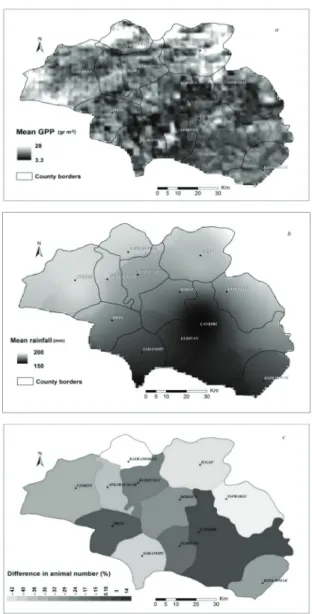
The 10 year figures illustrated the least production was observed in both central and southern region of the province (Figure 4a). Field surveys showed that the rangelands were mostly covered by stones and the plants were of a steppe character resulting in very low canopy cover. On the other hand, in the northern part and northwest regions of Çerkeş and Ilgaz counties, the rangelands produced greater biomasses than the rest of the region (Figure 4a). Ranges in these regions were calculated to have higher canopy covers and Table 2- Modelled monthly and annual summed GPP

Çizelge 2- Aylık ve yıllık toplam GPP

GPP (ton) Months 2000 2001 2002 2003 2004 2005 2006 2007 2008 2009 March 156 223 96 228 261 300 303 54 113 142 April 2484 2347 2044 2090 2038 1840 3342 2992 1839 1525 May 15439 4204 7765 7478 9873 7528 7038 5720 5782 6681 June 17688 4076 6492 6987 7322 8027 5871 3912 6227 3659 July 1665 249 572 502 655 789 92 146 375 529 August 269 62 121 95 151 137 3 22 52 100 TOTAL 37701 111618 170906 173801 203004 186214 166490 128463 14388 12636

(7)

561

Ta r ı m B i l i m l e r i D e r g i s i – J o u r n a l o f A g r i c u l t u r a l S c i e n c e s 22 (2016) 555-565 dry yields which was confirmed with the field survey

results. The differences in 10 year average production may be resulted from the changes in the amount of rainfall and the frequency of animal grazing. The average rainfall during growing season (throughout 2000-2009) was 156 mm, which explains the low yield in the southern and eastern regions. However in the northern parts of the province, where the yield was relatively higher, average rainfall was 200 mm. This situation supported the general conclusion that the higher rainfall is, the more biomass the plant produce (Figure 4a and 4b).

The number of grazing animals can be another factor effecting variation in biomass production. There was a gradual decrease in the animal number for 9 year-period of 2000-2008 (Figure 5). Unfortunately, there weren’t any statistical records of number of grazing animals for the 2009. In the 9 years, the total number of ruminants has been decreased by 21.347% totaling to 90539 in 2008 (Table 3). Figure 4c shows percentage change of the animal number with respect to the province’s counties. Positive variations in the period explained the increases in animal number, while negatives indicated the decreases. The animal numbers decreased in 9 out of 12 counties, but increased in 3 counties (Figure 4c).

It was seen that average GPP was higher in the counties which had negative variations in the number of animal than those which had positive variations. Besides, the northern counties (Çerkes, Bayramören, Ilgaz, Kurşunlu and Atkaracalar) had higher GPP values as a result of higher amount of precipitation (Figure 4b) compared to the southern counties and lower number of grazing animals resulting in lower grazing pressures on the live vegetation. The results showed both rainfall and animal number exhibited an interactive role in rangelands’ production.

3.2. Evaluation of model performance

Model performance was tested to determine how well the LUE model estimated the GPP of rangelands. Two approaches were used for performance evaluation; a) comparison of field biomass measurements with the LUE model’s GPPs and b) regression analysis between integrated

normalized difference vegetation index (INDVI) and LUE model’s GPPs.

Relationships between field measurements of biomass and LUE model GPPs were tested by Figure 4- a, average GPP; b, average rainfall; c, animal number variation for 10 years (2000-2009) by counties

Şekil 4- a, 10 yıllık ortalama GPP üretimi; b, ortalama yağış; c, ilçelere göre hayvan sayısındaki 10 yıllık varyasyon

(8)

562

Ta r ı m B i l i m l e r i D e r g i s i – J o u r n a l o f A g r i c u l t u r a l S c i e n c e s 22 (2016) 555-565 correlation analysis for both years. There were

moderate correlations between variables (r= 0.60 and r= 0.41 for 2008 and 2009, respectively). The relationships were insignificant for both years (P>0.05). Unfortunately the correlations were not very high because of the various factors such as sampled plant types, scale differences between sampling area

and pixel size of satellite image, and measurement errors. The sampled plant type was the most important factor making the biomass measurements inconsistent. For instance, herbaceous plants (Festuca sp., Poa sp.,

Bromus sp.) had high ground coverage due to their

extensive spread habit causing high NDVI values which drove the model to calculate higher GPPs than the that of woody plants such as thyme (Thymus sp.), and astragalus (Astragalus sp.). Scale differences caused location errors between ground observations and satellite data (NDVI) and thus low correlations, because biomass measurements were taken from very small site (1 m2_{) which was approximately}

1/1.000.000 of one pixel size of NDVI data.

The second method for model evaluation was the use of INDVI accounting for the summed NDVI of during growing stage. The INDVI was regressed with the GPPs calculated from the LUE model (LUE-GPPs). The correlation was significantly high (r= 0.83) by giving the regression coefficient of 0.69 which means that approximately 69% of total variation in the LUE-GPPs can be explained by the linear relationship between these variables (Figure 6). Significance test of regression explained that there was a relationship between the variables in the linear regression model (t= 7.4, P<0.05). According to ANOVA test, the INDVI and the LUE-GPP were statistically significant (Table 4).

LUE model GPP

s (

g m

-2)

INDVI

Figure 6- Correlation between INDVI and LUE model GPPs

Şekil 6- INDVI ve LUE modeli GPP arasındaki korelasyon

9

Figure 5- The number of animal between 2000-2008 in Çankırı province (TUIK 2009)

Şekil 5- 2000-2008 yılları arası Çankırı ilindeki hayvan sayısı (TUIK 2009)

Table 3- The number of animals based on counties in 2000 and 2008 (TUIK 2009)

Çizelge 3- 2000 ve 2008 yıllarındaki ilçelere göre hayvan sayısı (TUIK 2009) Counties The number of animal ₂₀₀₀ ₂₀₀₈ Difference _(%)*

Atkaracalar Bayramören Çerkeş Eldivan Ilgaz Kızılırmak Korgun Kurşunlu Merkez Orta Şabanözü Yapraklı Total 4438 3609 24808 3218 11572 9759 5265 9425 14337 9439 9900 9340 115110 3011 2092 17463 3224 7095 7350 4335 7986 16360 9766 6324 5533 90539 -32.15 -42.03 -29.60 0.18 -38.68 -24.68 -17.66 -15.26 14.11 3.46 -36.12 -40.76 -21.34

*_{, positive variations in the period explained the increases in animal number, while negatives indicated the decreases.} 3.2. Evaluation of model performance

Model performance was tested to determine how well the LUE model estimated the GPP of rangelands. Two approaches were used for performance evaluation; a) comparison of field biomass measurements with the LUE model’s GPPs and b) regression analysis between integrated normalized difference vegetation index (INDVI) and LUE model’s GPPs.

Relationships between field measurements of biomass and LUE model GPPs were tested by correlation analysis for both years. There were moderate correlations between variables (r= 0.60 and r= 0.41 for 2008 and 2009 respectively), the relationships were insignificant for both years (P>0.05). The correlations weren’t very high because of the various factors such as sampled plant types, scale differences between sampling area and pixel size of satellite image, and measurement errors. The sampled plant type was the most important factor making the biomass measurements inconsistent. For instance, herbaceous plants (Festuca sp., Poa sp., Bromus sp.) had high ground coverage due to their extensive spread habit causing high NDVI values which drove the model to calculate higher GPPs than the that of woody plants such as thyme (Thymus sp.), and astragalus (Astragalus sp.). Scale differences caused location errors between

80000 85000 90000 95000 100000 105000 110000 115000 120000 2000 2001 2002 2003 2004 2005 2006 2007 2008 Th e Nu mb er o f A nimal Years

The Number of Animal

Years

Figure 5- The number of animal between 2000-2008 in Çankırı province (TUIK 2009)

Şekil 5- 2000-2008 yılları arası Çankırı ilindeki hayvan sayısı (TUIK 2009)

Table 3- The number of animals by counties in 2000 and 2008 (TUIK 2009)

Çizelge 3- 2000 ve 2008 yıllarında ilçelere göre hayvan sayısı (TUIK 2009)

Counties The number of animal₂₀₀₀ ₂₀₀₈ Difference _(%)*

Atkaracalar Bayramören Çerkeş Eldivan Ilgaz Kızılırmak Korgun Kurşunlu Merkez Orta Şabanözü Yapraklı Total 4438 3609 24808 3218 11572 9759 5265 9425 14337 9439 9900 9340 115110 3011 2092 17463 3224 7095 7350 4335 7986 16360 9766 6324 5533 90539 -32.15 -42.03 -29.60 0.18 -38.68 -24.68 -17.66 -15.26 14.11 3.46 -36.12 -40.76 -21.34

*_{, positive variations in the period explained the increases in} animal number, while negatives indicated the decreases.

(9)

Uydu Verisi ve AgrometShell Modülü ile Işık Kullanım Etkinliği (LUE) Modeli Kullanarak Çankırı İli Meralarının..., Ünal & Bayramin

563

3.3. Sensitivity analysis of the model

Sensitivity analysis was performed to determine to what extent the choice of variables affected the model output. There is a large body of scientific literature on various methods of sensitivity analysis (Morgan & Henrion 1990; Shevenell & Hoffman 1993). Of the approaches for sensitivity analysis, no single method serves as the best analysis for all modelling efforts. The sensitivity ratio, also known as elasticity equation, is used for the analysis in this study (Anonymous 2001). The sensitivity ratio (SR) shown in Equation 9 is the percentage change in output divided by the percentage change in input for a specific input variable. When the sensitivity ratio is higher, the more sensitive the model output is.

10

data.

The second method for model evaluation was the use of INDVI accounting for the summed NDVI of during growing stage. The INDVI was regressed with the GPPs calculated from the LUE model (LUE-GPPs). The correlation was significantly high (r= 0.83) by giving the regression coefficient of 0.69 which means that approximately 69% of total variation in the LUE-GPPs can be explained by the linear relationship between these variables (Figure 6). Significance test of regression explained that there was a relationship between the variables in the linear regression model (t= 7.4, P<0.05). According to ANOVA test, the INDVI and the LUE-GPP were statistically significant (Table 4).

Figure 6- Correlation between INDVI and LUE model GPPs

Şekil 6- INDVI ve LUE modeli GPP arasındaki korelasyon

Table 4- Significance test statistics for linear regression of INDVI and model GPP

Çizelge 4- INDVI ve model GPP arasındaki doğrusal regresyonun anlamlılık testi

df SS MS F Significance F

Regression 1 371.75 371.75 55.40 0.00 Residual 25 167.73 6.70

Total 26 539.49

Coefficients Standard error t Stat P-value

Intercept -2.39 1.57 -1.52 0.14 INDVI 3.74 0.50 7.44 0.00

3.3. Sensitivity analysis of the model

Sensitivity analysis was performed to determine to what extent the choice of variables affected the model output. There is a large body of scientific literature on various methods of sensitivity analysis (Morgan & Henrion 1990; Shevenell & Hoffman 1993). Of the approaches for sensitivity analysis, no single method serves as the best analysis for all modelling efforts. The sensitivity ratio, also known as elasticity equation, is used for the analysis in this study (Anonymous 2001). The sensitivity ratio (SR) shown in Equation 9 is the percentage change in output divided by the percentage change in input for a specific input variable. When the sensitivity ratio is higher, the more sensitive the model output is.

1 1 2 1 1 2 x x x y y y SR (9)

Where; SR, sensitivity ratio; x1, average value calculated from the 10 year data of model variables (FPAR, PAR and ɛ); x1 value for the LUE variable was taken as 0.500 approximating the average of highest and lowest values for the short grass steppe (Table 1); x2, can take values of x1 variable’s minimum and maximum values for the “worst” and “best” case scenarios, respectively; y1, represents the average GPP

(9) Where; SR, sensitivity ratio; x1, average value calculated from the 10 year data of model variables (FPAR, PAR and ɛ); x1 value for the LUE variable was taken as 0.500 approximating the average of highest and lowest values for the short grass steppe (Table 1); x2, can take values of x1 variable’s

minimum and maximum values for the “worst” and “best” case scenarios, respectively; y1, represents the average GPP calculated from variables’ means;

y2, represents the GPP calculated from the variables

one of whose value is changed in accordance with scenarios. The minimum and maximum values of the stated variables were used to build “Best Case” and “Worst Case” scenarios for calculation of sensitivity ratios (Table 5). Best and worst case scenarios respectively denote minimum and maximum GPP to be produced, which is directly proportional to degree of variables in GPP equation. The minimum and maximum values of FPAR, PAR and ɛ variables were derived from 10 year grid data used, while the minimum and maximum LUE values were directly taken from empirical measurements given in the Table 1 (Sims & Singh 1978).

For the worst case scenario, all variables have the SR value of around 1.00, which means that biomass produced is dominated by all variables almost equally (Table 5). As for the best case scenario, similar results were obtained that SR values are smaller than 1.00 but around it. The most sensitive variable is FPAR (SR= 0.99). It is because the FPAR Table 4- Significance test statistics for linear regression of INDVI and model GPP

Çizelge 4- INDVI ve modelin ürettiği GPP arasındaki doğrusal regresyonun anlamlılık testi

df SS MS F Significance F

Regression 1 371.75 371.75 55.40 0.00 Residual 25 167.73 6.70

Total 26 539.49

Coefficients Standard error t Stat P-value

Intercept -2.39 1.57 -1.52 0.14 INDVI 3.74 0.50 7.44 0.00

Table 5- Sensitivity ratios (SR) for LUE model variables for the best case and the worst case scenarios

Çizelge 5- En iyi ve en kötü senaryolara göre LUE modeli değişkenlerinin hassasiyet oranı (SR)

Worst case scenario Best case scenario

Variables X1 X2 Y1 Y2 SR X1 X2 Y1 Y2 SR FPAR 0.261 0.003 0.592 0.0043 1.00 0.261 0.588 0.592 1.330 0.99 PAR 8.660 6.050 0.592 0.4101 1.02 8.660 10.915 0.592 0.741 0.96 ɛ 0.529 0.061 0.592 0.0666 1.00 0.529 0.979 0.592 1.082 0.97 LUE 0.500 0.420 0.592 0.4883 1.01 0.505 0.620 0.592 0.720 0.94

(10)

564

Ta r ı m B i l i m l e r i D e r g i s i – J o u r n a l o f A g r i c u l t u r a l S c i e n c e s 22 (2016) 555-565 is positively related to the vegetation index which is

an estimate of how much photosynthetically active vegetation is present. As a general conclusion for sensitivity analysis, the variables are each important factors affecting biomass production and this conclusion is supported by high SR values.

4. Conclusions

This study combines the outputs of AgrometShell module and satellite NDVI data using the LUE model approach to estimate annual GPP of Çankırı rangelands. The 10-year average modelled GPPs point out that annual production was approximately 17880 tons which corresponds to 11.4 g m-2_{of dry}

yield. The GPP production of the region varied seasonally and annually. The main reasons of this variability were rainfall and the number of animals grazed.

Comparison of model results of annual primary production (GPP) with ground truthing showed that the model unfortunately did not produce significant correlations (P>0.05) due to several sources of uncertainty and inconsistencies such as sampled plant types, erratic LUE values, residues’ background effect, estimation of incident PAR and scale differences between satellite data and ground sample size. On the other hand, integrated NDVI approach produced higher correlation (r= 0.83, P<0.05) between the LUE model GPP output and the INDV values. According to sensitivity analysis, the model variables almost equally affect the GPP production in the worst case scenario. On the other hand the FPAR variable was the most significant factor affecting the biomass production in the best case.

The main advantage of the model used in this study was that it simulates primary production by considering the water used by plants (actual transpiration), which was difficult parameter to measure needing extensive ground based measurement equipment. However, AgrometShell module used here easily calculated this parameter through the weather data.

The results are encouraging that the LUE model could be applied in any rangeland region where conventional weather and satellite NDVI data exist. On the other hand, accurate estimation of GPP over large areas as rangelands, pastures, and forest does still have some drawbacks such as the effects of varying environmental conditions on vegetation canopy reflectance issues and the estimation of empirical LUE factor and other stress factors. It is apparent that GPP modelling studies will be active research area in future to overcome those handicaps.

Acknowledgements

This research study was supported by the project (No: 106G017) of “National Rangeland Management” funds of the Scientific and Technological Research Council of Turkey (TUBITAK). We express our gratitude to all staff for helping during the field visit and office work.

References

Allen R G, Pereira L S, Raes D & Smith M (1998). Crop Evapotranspiration: Guidelines for Computing Crop Water Requirements. United Nations Food and Agriculture Organization (FAO), Irrigation and Drainage Paper 56, Rome, Italy

Anonymous (2001). Risk assessment guidance for superfund (RAGS). In: Volume III-Part A. Process for Conducting Probabilistic Risk Assessment. U.S. Environmental Protection Agency Washington, DC, pp. 385-387

Anonymous (2012). Ulusal Mera Kullanım ve Yönetim Projesi sonuç raporu. Proje No: 106G017. TÜBİTAK Kamu Kurumları Araştırma ve Geliştirme Projelerini Destekleme Programı (1007 Programı)

Brogaard S, Runnström M & Seaquist J A (2004). Primary production of inner Mongolia, China between 1982 and 1999 estimated by a satellite-driven light use efficiency model. Global and Planetary Change 45:

313-332

Goetz S J, Prince S D, Goward S N, Thawley M M & Small J (1999). Satellite remote sensing of primary production: an improved production efficiency modelling approach. Ecological Modelling 122:

(11)

565

Ha W, Gowda P, Oommen T, Marek T, Porter D & Howell T (2011). Spatial interpolation of daily reference evapotranspiration in the Texas High Plains. In: World Environmental and Water Resources Congress, May 22-26, Palm Springs, CA, pp. 2796-2804

Hilker T, Nicholas C C, Wulder M A, Black T A & Guy R D (2008). The use of remote sensing in light use efficiency based models of gross primary production: A review of current status and future requirements.

Science of the Total Environment 404: 411-423

Holben B N (1986). Characteristics of maximum-value composite images from temporal AVHRR data.

International Journal of Remote Sensing 7:

1417-1434

Huete A, Didan K, Miura T & Rodriguez E (2002). Overview of the radiometric and biophysical performance of the MODIS vegetation indices.

Remote Sensing of Environment 83: 195-213

Ketenoğlu O, Quezel P, Akman Y & Aydoğdu M (1983). New syntaxa on the gypsaceous formation in the Central Anatolia. Ecologia Mediterranea 9(3-4):

211-221

Kurt L, Tuğ G N & Ketenoğlu O (2006). Synoptic view of the steppe vegetation of Central Anatolia (Turkey).

Asian Journal of Plant Sciences 5(4): 733-739

Le Roux H X, Gauthier A, Begue H & Sinoquet H (1997). Radiation absorption and use by humid savannah grassland: assessment using remote sensing and modelling. Agricultural and Forest Meteorology 85:

117-132

Los S O, North P R J, Grey W M F & Barnsley M J (2005). A method to convert AVHRR normalized difference vegetation index time series to a standard viewing and illumination geometry. Remote Sensing

of Environment 99(4): 400-411

Mermer A, Ünal E, Aydoğdu M, Urla Ö, Yıldız H & Torunlar H (2012). Determining rangeland areas by satellite images. TABAD-Research Journal of

Agricultural Sciences 5: 107-110

Monteith J L (1972). Solar radiation and productivity in tropical ecosystems. Journal of Applied Ecology 9:

747-766

Morgan G M & Henrion M (1990). Uncertainty: A Guide to Dealing with Uncertainty in Quantitative Risk and Policy Analysis. Cambridge University Press, NY Mukhala E & Hoefsloot P (2004). AgrometShell

Manual. Agrometeorology Group, Environment and Natural Resources Service, Food and Agricultural Organization Rome, Italy

Prince S D (1991). Satellite remote sensing of primary production: comparison of results for Sahelian grasslands 1981-1988. International Journal of

Remote Sensing 12: 1301-1311

Seaquist J W, Olsson L & Ardö J (2003). A remote sensing based primary production model for grassland biomes.

Ecological Modelling 169: 131-155

Shevenell L & Hoffman F O (1993). Necessity of uncertainty analyses in risk assessment. Journal of

Hazardous Materials 35: 369-385

Sims P L & Singh J S (1978). The structure and function of ten western North America grasslands. II. Intra-seasonal dynamics in primary producer compartments.

Journal of Ecology 66: 251-285

Tucker C J, Vanpraet C, Boerwinkel E & Gaston A (1983). Satellite remote sensing of total dry matter production in the Senegalese Sahel. Remote Sensing

of Environment 13: 461-474

TUIK (2009). Livestock statistics. Retrieved in July, 18 2009 from http://www.tuik.gov.tr

Uzun B & Demir V (2012). Fotosentetik aktif radyasyon (FAR) ölçümlerinde LED ve foto diyotların hassas tarım açısından kullanılabilirliği üzerine bir araştırma. Tarım Bilimleri Dergisi-Journal of Agricultural

Sciences 18 (3): 214-225

Wight J R & Hanks R J (1981). A water-balance, climate model for range herbage production. Journal of Range