Artificial Neural Network Approaches For Inflow Estimation At Adiguzel Dam, Turkey

©BEYKENT UNIVERSITY

ARTIFICIAL NEURAL NETWORK

APPROACHES FOR INFLOW ESTIMATION AT

ADIGÜZEL DAM, TURKEY

Mahmut FIRAT

Pamukkale University, Civil Engineering Department, 20017, Denizli, Türkiye,

mfirat@pau.edu.tr

Received: 02 May 2008, Accepted: 09 May 2008

ABSTRACT

Accurate modeling and forecasting of hydrological processes such as rainfall, rainfall-run off relationship, runoff, is important for management and planning of water resources. In this study, applicability of Artificial Neural Network (ANN) methods for inflow forecasting at Adıgüzel dam on the Büyük Menderes River catchment was investigated. For this purpose, daily river flow data points were obtained from two river flow gauge stations on the Büyük Menderes river, Çıtak Köprü (713), Dört Değirmen (735), over 12 years, 1988 - 2000, and models having various input structures were constructed. The two different types of ANN, Feed Forward Neural Networks and Radial Basis Neural Networks, have been used to forecast daily river flow. The models were trained and tested by FFNN and RBNN and the results of models were compared with field observation data. Criteria for performance evaluation were identified in order to evaluate and compare the performances of FFNN and RBNN models. Then the best fit model and network structure were determined according to these criteria.

Keywords: Inflow, ANN, Feed Forward Neural Networks, Radial Basis Neural Networks, Adıgüzel Dam, Büyük Menderes Catchment.

ADIGÜZEL BARAJINDA GİREN AKIM

TAHMİNİ İÇİN YAPAY SİNİR AĞ

YAKLAŞIMLARI

ÖZET

Yağış, yağış-akış ilişkisi ve akış gibi hidrolojik olayların doğru ve güvenilir bir şekilde modellenmesi ve tahmin edilmesi su kaynaklarının planlanması ve yönetilmesinde oldukça önemlidir. Bu çalışmada, Yapay Sinir Ağlarının

(YSA) Büyük Menderes havzasında yer alan Adıgüzel barajına giren akımların tahmin edilmesinde uygulanabilirliliği araştırılmaktadır. Bu amaçla, Adıgüzel barajı menbasında yer alan B. Menderes Çıtak Köprü (713), Dört Değirmen (735) istasyonlarında 1988-2000 yılları arasında ölçülmüş günlük akış verileri alınmış ve farklı giriş yapısına sahip modeller kurulmuştur. Baraja giren akımların tahmin edilmesinde İleri Beslemeli Sinir (İBYSA) ve Radial Tabanlı Sinir Ağları (RTSA) kullanılmaktadır. Kurulan modeller İBYSA ve RTSA ile eğitilerek denenmiş ve sonuçları gözlem sonuçları ile karşılaştırılmıştır. Modellerin başarımlarını değerlendirmek amacıyla çeşitli performans değerlendirme ölçütleri hesaplanmıştır. Daha sonra bu sonuçlara göre en uygun model yapılarına karar verilmiştir.

Anahtar Kelimeler: Giren Akım, YSA, İleri Beslemeli Sinir Ağları, Radial Tabanlı Sinir Ağları, Adıgüzel Barajı, Büyük Menderes havzası.

1. INTRODUCTION

In modeling hydrological processes, the measurement of natural phenomena is firstly necessary. In order to estimate the hydrological processes such as precipitation, runoff, and fluctuation of water level by using existing methods, some parameters such as physical properties of the watershed or region and observed detailed data are necessary. The Büyük Menderes River catchment, located in the west of Turkey, is one of the most important fresh water resource in Turkey. In this region, the Büyük Menderes River has a quite significant impact on drinking water, irrigation and hydroelectric energy supplies. River water level fluctuations depend on the main several impacts as climatic and hydro-meteorological variables of the lake basin, anthropogenic effects of human activities, water usage for agricultural and hydroelectric energy. In the face of these impacts, forecasts of future river flow can be helpful in making efficient operating decisions of water demand, for the wise and sustainable use of river. In last decades, new methods called artificial intelligence techniques are used for modeling of the nonlinear and complex systems. ANN are used in the estimation of the values of variables in hydrologic and hydro mechanical modeling such as daily and monthly flow volume, flow rate, temperature and snow melting, suspended materials. Some specific applications of ANN to hydrology include modeling rainfall-runoff process [1, 2, 3, 4], river flow forecasting [5, 6], hydrologic time series modeling [7], sediment transport prediction [8, 9, 10, 11], reservoir operation

[12], sediment concentration estimation [13], and ground water modeling [14]. In addition, in the literature many studies were carried out by RBNN methods for modeling and forecasting of hydrological processes. These are rainfall -runoff modeling [15], sediment transport prediction [16]. Moreover, The ASCE Task Committee reports (2000) have realized a comprehensive review of the applications of ANN in the hydrological forecasting context [17].

In this study, the applicability of ANN for inflow forecasting at Adıgüzel dam on the Büyük Menderes River catchment was investigated. For this aim, two

stations, B. Menderes Çıtak Köprü (713) and Dört Değirmen (735), located upstream of the dam are selected and daily river flow data was obtained from flow gauging stations at period 1988-2000 years. The models having various input variables were constructed and trained by Feed Forward Neural Network (FFNN) and Radial Basis Neural Networks (RBNN). The results of FFNN and RBNN methods were compared with field observation data and the best-fit model structure is determined according to some statistical criteria.

2. ARTIFICIAL NEURAL NETWORKS

Artificial Neural Networks (ANN) is a method developed and based on the biological neural system. An ANN consists of many elements called neurons that are joined parallel and having a non-linear structure [18]. In literature, there are various types of artificial neural networks. These are Feed Forward Neural Networks (FFNN), Feed Back Neural Networks and Radial Basis Neural Network (RBNN) [11, 19]. In this study, FFNN and RBNN methods were used for inflow forecasting at Adıgüzel dam.

Feed Forward Neural Networks (FFNN)

A FFNN consists of at least three layers: input layer, output layer and hidden layer. The numbers of input and output neurons in input and output layers are determined according to the conditions of the evaluated problem. On the other hand, the numbers of hidden neurons and hidden layers are selected by trial and error method during training process [2, 19]. Figure 1 shows the mathematical model of a neuron. The output of network is calculated by passing the summation function from the activation function of the neuron.

N Ynet = 2 Xi w + w0 (1) i=1 N Yout = f (Ynet) = f ( £ Xi w + w0) (2) i=1

Where, Yout is the result of neural network, J net is the activation function, Ynet is summation function, Yi is the input variable, wi is the weight coefficient of each input neuron and w0 is the bias.

•Y Y

Input Layer Hidden Layer Output Layer Figure 1. Mathematical Model of Neuron

As the neural networks are ultimately based on biologic neural networks, they are trained by means of real world samples. In general, learning may be grouped into two parts: as supervised learning and unsupervised learning. In the supervised learning, input and output data is fed to the neural network and the network is asked to generate weight coefficients according to these data and solve the problem. In unsupervised learning, only input variables are given to the neural network and weight coefficients are determined according to this [11]. In this study, the back propagation-learning algorithm, supervised learning, and tangent activation function have been used for training of FFNN models.

The summation function obtained by Equation 1 is applied to the chosen non-linear transfer function and the output of the network is determined. Then the results of the network are compared with the real results and the network error is calculated with Equation 4,

where: Jr is the error between observed value and network result, Yobs is observation output value. The training process continues until this error reaches an acceptable value.

Radial Basis Neural Networks (RBNN)

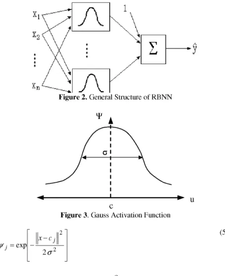
A RBNN has the structure of a feed forward network, which is trained by supervised learning. Several published studies describe the use of RBNN for pattern recognition and modeling of time series etc. Figure 2 shows a RBNN model having an input layer, an output layer and one hidden layer [15, 16]. The input data are presented to the network in an input layer and these data are

1

Yout = f (Ynet) = —

1 + e

transferred to a hidden layer by a non-linear activation function. The response of the network is obtained in the output layer.

The performance of RBNN depends on the center values. The various types of non-linear activation functions can be used for transferring of the input data to hidden layer. In this study, Gaussian activation function (the most commonly used) is selected as an activation function for training the data set [19]. The Gauss activation function is shown in Figure 3 and mathematical structure of this function is demonstrated in equation (5)

Figure 2. General Structure of RBNN

¥

u

Y j = exp x - c. 2a2

(5)

Where, x is the input sets of training, j is center values, and & is variance. The variance and center determine the properties of each function during the training process. The response of each hidden unit is scaled by its connecting

c

weights to the output units and then summed to produce the overall network output [19]. The response of the network is calculated by equation (6).

N (6)

yk = w0 +

X

V • (x) w jk

where, 1 is response of the jth hidden neuron, 1 is the weight coefficient between (j) the hidden unit and (k)th output unit, and W o is the bias. RBNN has just one hidden layer and the numbers of hidden neurons in this layer is determined by input data set length. The location of the first center may be chosen from the training data set, and the standard deviation (i.e. width) of the jth neuron is;

a = " m a x ( 7 ) i +1 ! k (8) 1 ^ 2 J r = " 2 ' ^ ( yobs - y net) 2 M

d y

where, m a x is maximum distance between training data set, net is response of the network, yobs is observation value. The training process continues until this error reaches an acceptable value.

3. STUDY AREA AND AVAILABLE DATA

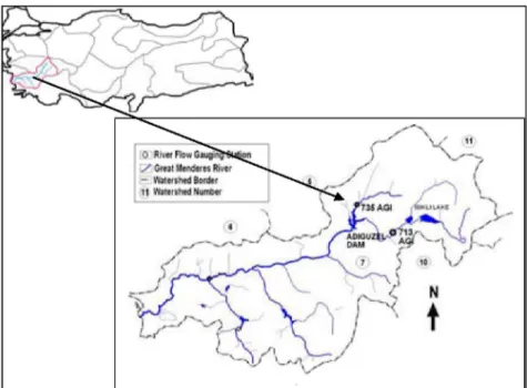
To illustrate the applicability and capability of the ANN method for inflow forecasting, the Büyük Menderes River, located in the west of Turkey, was chosen as a case study area. It has been operated for irrigation, hydropower generation, domestic use and recreation facilities. Figure 4 shows the study area and the locations of two river flow gauging stations, B. Menderes Çıtak Köprü (713) and Dört Değirmen (735), which are located upstream of Adıgüzel dam.

Figure 4. Büyük Menderes River and its drainage area

4. MODELING OF INFLOW BY ANN

A sufficient number of values in a data set is required at the training phase because the artificial neural networks are also trained with examples, as in the training of people. In total, 4383 daily river flow data points were obtained from river flow stations, B. Menderes Çıtak Köprü (713), Dört Değirmen (735) over 12 years, period 1988 - 2000. The statistical parameters, minimum value;

— —

s

m i n , maximum value; m a x , mean; x , standard deviation; x , variation

c c

coefficient v—, skewness coefficient; s— for the total observed daily data sets are given in Table 1.

Table 1: Statistical parameters for data sets

Variable x min xm a x x ¿x c

ß ( i )7 1 3 (m3/s) 0.056 32.800 6.623 7.846 1.381

0(0735 (m3/s) 1.61 69.90 5.35 4.65 3.82

One of the most important steps in developing a satisfactory forecasting model is the selection of the input variables. Hence, Pearson and Spearman correlation coefficients between input and output variables were calculated in order to establish the models. Different combinations of the antecedent flows

were used to construct the appropriate input structure in the forecasting models. The general structures of the forecasting models for two stations are given in Equation (9) and (10), respectively. The structures of the models are shown in Table 2 and Table 3.

R-713 M Model: _{ß(0713 = f (Q(t-1)713, Q(t - n)713)} (9)

R-735 M Model: Q(t)735 = f(Q(t-1)735 Q(t-n)713) (10)

Table 2. The models for river flow station of Çıtak Köprü (713)

Model Input structure Output

R-713 M1 Q(t -1)713

Q(t

Q(t - 1)713 Q(t -

Q(t

Q(t - 1)713 Q(t -

Q(t

Q(t

Q(t

Q(t - 1)713 Q(t -

Q(t

Q(t - 1)713 Q(t -

Q(t

Table 3. The models for river flow station of Dört Değirmen (735)

Model Input structure Output

R-735 M1 Q(t -1)735 Q(t)735 R-735 M2 Q(t -1)735 Q(t - 2 )735 Q(t)735 R-735 M3 Q(t -1)735 Q(t - 2)735 Q(t - 3 )7 3 5 _Q(t)735 R-735 M4 Q(t -1)735 Q(t - 2)735 Q(t -3)735 Q(t - 4 ) 735 _Q(t)735 R-735 M5 Q(t -1)735 Q(t - 2)735 Q(t -3)735 Q(t -4)735 Q(t -5)735 Q(t)735 R-735 M6 Q(t -1)735 Q(t - 2)735 Q(t -3)735 Q(t -4)735 Q(t -5)735 Q(t - 6 )735 Q(t)735

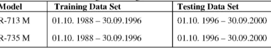
Where; Q t represents the river flow at time (t), Q ( ), . . . Q ( t n are the river flow respectively at times (t-1) ... (t-n). The river flow data of 713 and 735 stations were divided into two subgroups, training and testing set, for training and testing of R-713 M and R-735 M ANN models. The training data set includes total 2922 daily data at period 1988-1996 and testing data set has total 1461 daily data (at period 1996-2000 year). The structures of data sets of R-713 M and R-735 M models are given in Table 4.

Table 4: Structure of training and testing data sets

Model Training Data Set Testing Data Set

R-713 M R-735 M 01.10. 1988 - 30.09.1996 01.10. 1988 - 30.09.1996 01.10. 1996 - 30.09.2000 01.10. 1996 - 30.09.2000

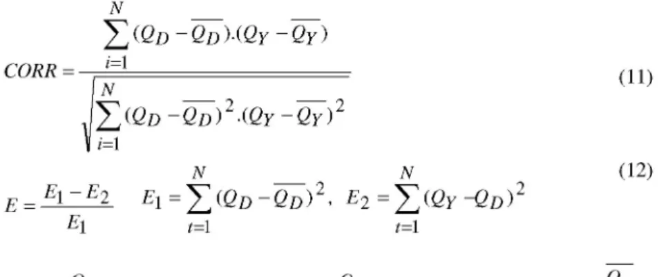
The numbers of hidden neurons in hidden layer, learning rate, momentum coefficient, and epoch are determined by trial and error method during the training processes. The performances of the models used in both the training and the testing of data are evaluated and the best training/testing data set is selected according to Correlation Coefficient (CORR), Efficiency (E) and Root Mean Square Error (RMSE).

N CORR = 2 (QD - QD ).(QY - QY ) i=1

il

2 (Qd - QD )

.(QY - QY )

= 2

)

,

= 2 (Qy

)

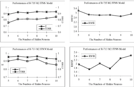
Where, Q y is the estimated river flow, Q d is the observed river flow, Q y is the average of the estimated flows, Q d is the average of the observed flows. Figure 5 shows the performances of R-713 M and R-735 M models. The best-fit input structures of R-713 M and R-735 M FFNN models are determined according to these criteria.

Comparing of the performances of the R-713 M FFNN models, the lowest value of RMSE and the highest values of the E and CORR are obtained from R-713 M2 FFNN model having two input variables. On the other hand, comparing the results of R-735 M FFNN models, the performance of R-735 M2 FFNN, which has also two input variables, is better than other models. As a result, R-713 M2 and R-735 M2 FFNN models are selected as the best-fit models for inflow forecasting at Adiguzel dam according to the statistical criteria presented in Figure 5. The number of hidden layers, the hidden neurons in these layers and training parameters of these models were determined by trial and error method. The performances of the best fit R-713 M2 and R-735 M2 FNN models are shown in Figure 6.

Performances of R-735 M2 FFNN Model Performances of R-735 M2 FFNN Model

6 7 8 9 The Numbers of Hidden Neurons

6 7 8 9 T he Numbers of Hidden Neurons

Performances of R-713 M2 FFNN Model

5 6 7 8 9 10 The Numbers of Hidden Neurons

Performances of R-713 M2 FFNN Model 2.6 2.4 q 2.2 -; 2 " 1.8 1.6 -1.4 5 6 7 8 9 The Numbers of Hidden Neurons

Figure 6: Performances of R-713 M2 and R-735 M FFNN models

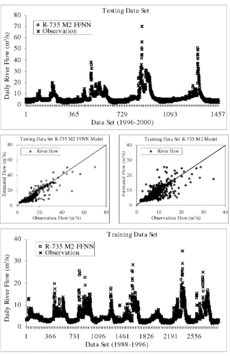
As can be seen in Figure 6, the best-fit training parameters of the R-713 M2 FFNN model were obtained as the numbers of hidden neurons (6), learning rate (0.01), momentum coefficient (0.5) and epoch (1000). On the other hand, the training parameters of R-735 M2 FFNN models are numbers of hidden neurons (10), learning rate (0.05), momentum coefficient (0.6) and epoch (1500). The training and testing performances of the R-713 M2 and R-735 M2 FFNN models are given in Figure 7 and Figure 8, respectively.

1.4

0.9 0.9

0.8 0.8

Testing Data Set

365 729 1093 Data Set (1996-2000)

1457

Testing Data Set R-713 M2 FFNN Model

0 10 20 30 Observation Flow (m3/s)

40

Training Data Set R-713 M2 Model

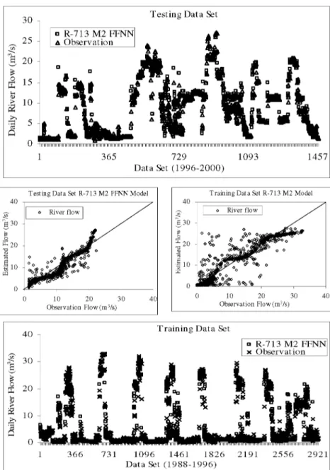
10 20 30 Observation Flow (m3/s) 4 0 T r a i n i n g D a t a Set • R - 7 1 3 M 2 F F N N x O b s e r v a t i o n 1 3 6 6 7 3 1 1 0 9 6 1 4 6 1 1 8 2 6 2 1 9 1 2 5 5 6 2 9 2 1 D a t a Set ( 1 9 8 8 - 1 9 9 6 )

Figure 7 : Comparison of the results R-713 M 2 F F N N and Observation

Testing Data Set R-735 M2 FFNN Model

0 20 40 60 80 Observation Flow (m3/s)

Training Data Set R-735 M2 Model

0 10 20 30 40 Observation Flow (m3/s)

Training Data Set • R-735 M2 FFNN

x Observation

1 366 731 1096 1461 1826 2191 2556 Data Set (1988-1996)

Figure 8 : Comparison of the results R-735 M2 FFNN and Observation

In order to get more reliable and accurate comparison, the best-fit models are also trained and tested by RBNN method. Comparison of performances of FFNN and RBNN models are shown in Table 5.

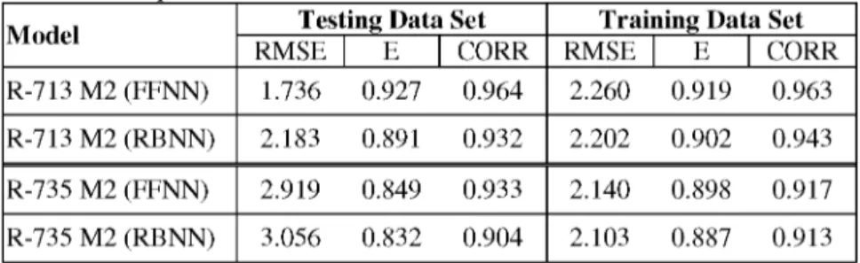
Table 5: Comparison of Performances of FFNN and RBNN Models

Model Testing Data Set Training Data Set

Model

RMSE E CORR RMSE E CORR

R-713 M2 (FFNN) 1.736 0.927 0.964 2.260 0.919 0.963

R-713 M2 (RBNN) 2.183 0.891 0.932 2.202 0.902 0.943

R-735 M2 (FFNN) 2.919 0.849 0.933 2.140 0.898 0.917

R-735 M2 (RBNN) 3.056 0.832 0.904 2.103 0.887 0.913

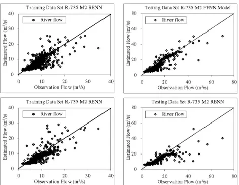
As can be seen in Table 5, the ANN models have been evaluated using their performance in training and testing sets. It appears that the ANN models are accurate, with all the values of RMSE are small, and all CORR and E values are also very close to unity. Comparing the results of the FFNN and RBNN models, it can be seen that the values of the RMSE of the FFNN model are lower than those of the RBNN model. In addition, the values of the E and CORR of the FNN model are higher than the RBNN model values. These results suggest that the FFNN and RBNN methods can be successfully applied to river flow estimation and modeling. The comparison of the results of the FFNN, RBNN models and observation are given in Figures 9 and 10.

Training Data Set R-735 M2 RBNN

0 10 20 30 40 Observation Flow (m3/s)

Training Data Set R-735 M2 RBNN

0 10 20 30 40 Observation Flow (m3/s)

Testing Data Set R-735 M2 FFNN Model

0 20 40 60 80 Observation Flow (m3/s)

Testing Data Set R-735 M2 RBNN

0 20 40 60 80 Observation Flow (m3/s)

Figure 10: Comparison of Results of RBNN Model and Observations

CONCLUSION

In this study, the applicability of ANN methods, FFNN and RBNN, for inflow forecasting at the Adıgüzel Dam on the Büyük Menderes River was investigated. Daily river flow data extended period 12 years were obtained from flow gauge stations B. Menderes Çıtak Köprü (713) and Dört Değirmen (735). Models with a range of input variables were developed for each station. These models were trained and tested by FFNN and RBNN methods and some statistical criteria to evaluate model performances evaluation were determined. It is concluded that the ANN model, in general, performs well for river flow estimation according to these statistical criteria. On the other hand, comparing the two forecasting models, it can be seen that the value of the RMSE of the FFNN model is lower than that of RBNN model. In addition, the values of the efficiency (E) and correlation coefficients (CORR) of the FNN model are higher than those of the RBNN model. The results have shown that ANN method can be successfully applied for inflow forecasting at the Adıgüzel Dam in the upper part of the Büyük Menderes catchment.

ACKNOWLEDGEMENT

The author is grateful for Editor and Anonymous Reviewers for their helpful and constructive comments on an earlier draft of this paper.

REFERENCES

Jeong, D., Kim, Y.O.; Rainfall-runoff models using artificial neural Networks for ensemble streamflow prediction, Hydrol. Process. 19, (2005), 3819-3835.

Kumar, A.R. Sudheer, K.P. Jain, S.K.Agarwal, P.K; Rainfall-runoff modelling using artificial neural Networks; comparison of network types, Hydrol. Process.19,(2005), 1277-1291.

Rajurkar, M.P., Kothyari, U.C. Chaube, U.C.; Modeling of the daily rainfall-runoff relationship with artificial neural network, Journal of Hydrology. 285, (2004), 96-113. Riad, S., Mania, J., Bouchaou, L., Nayyar, Y.; Rainfall-runoff model using an artificial neural network approach, Mathematical and Computer Modelling. 40, (2004), 839-846. Chang, F.J., Chang, L.C., Huang, H.L.; Real-time recurrent learning neural network for stream-flow forecasting, Hydrological Process. 16, (2002), 2577-2588.

Sudheer, K.P., Jain, A.; Explaining the internal behavior of artificial neural network river flow models, Hydrological Process. 18, (2004), 833-844.

Jain, A., Kumar, A.M.; Hybrid neural network models for hydrologic time series forecasting. Applied Soft Computing. 7, (2007), 585-592.

Agarwal, A., Mishra, S.K., Ram, S., ve Singh, J.K.; Simulation of runoff and sediment yield using artificial neural networks, Biosystems Engi. 94 (4), (1958), 597-613. Alp, M., Cigizoglu, H.K.; Suspended sediment load simulation by feed forward backpropagation method using hydrometeorological data, Environmental Modeling & Software. 22(1), (2007), 2-13.

Cigizoglu, H.K.; Estimation and forecasting of daily suspended sediment data by multi-layer perceptrons, Advances in Water Resources. 27, (2004), 185-195.

Fırat, M., Güngör, M.; Askı Maddesi Konsantrasyonu ve Miktarının Yapay Sinir Ağları ile Belirlenmesi, ÎMO Teknik Dergi, 15:(3), (2004), 3267- 3282.

Chang, Y.T., Chang, L.C., and Chang, F.J.; Intelligent control for modeling of real-time reservoir operation, part II: artificial neural network with operating rule curves, Hydrological Process. 19, (2005), 1431-1444.

Nagy H.M, Watanabe K, Hirano M.; Prediction of sediment load concentration in rivers using artificial neural network model, Journal of Hydr. Eng. 128, (2002), 588-595. Daliakopoulosa, I.N., Coulibalya, P., Tsanis, I.K.; Groundwater level forecasting using artificial neural networks, Journal of Hydrology. 309, (2005), 229-240.

Lin, G.F., Chen, L.H.; A non-linear rainfall-runoff model using radial basis function network, Journal of Hydrology. 289, (2004), 1-8.

Fırat, M., Güngör, M.; Radial tabanlı sinir ağları ile katı madde miktarının tahmini. II. Su Mühendisliği Sempozyumu, İzmir, (2005), 682-693.

ASCE Task Committee; Artificial neural networks in hydrology-II: Hydrologic applications. Journal of Hydrologic Engineering, ASCE 5 (2), (2000), 124-137.

Jang, J.S.R., Sun, C.T., Mizutani, E.; Neuro-Fuzzy and Soft Computing, Prentice Hall, ISBN 0-13-261066-3, 607 p., United States of America.(1997).