P O G L ilh ^ G
S £ S IE S A | ; p G S :O S S -S £ C T iG & ^ ^ iL · D
^ ^ ¿ A F P l I C A T I G ^ ^ . W ^ r l VACL l. i^... Z:-^· — rvi. i% r- >r\ ;vV G-> T'^ . - *» W’ <S wCJ o
A T H £ S :S
S U 3 M IT T S D TO 7 H E
A I^D G E A D U A T S S O r’iO w ^ u
'. i ri 5· r».i· r k>> T I” rU S I A i S S AOMmiSTEATfOiN^
0~ SSIOCE^T UK^^VEOSiTV
^ IN P A E T lA L F U L f lL L M S ^ T O ? T H E E£GUtaE(^;IEsMTS
F O E “O i E D S G E 2 E C 5
M A S T E R O F B U S f M E S S A D ?
l.
; S T P A T i
A . S w re y y « U r a l
E & b r u a r y 1 S 8 9
POOLING TIME SERIES AND CROSS-SECTIONAL DATA:
AN APPLICATION TO TURKISH EXPORT DEMAND ANALYSIS
A THESIS
SUBMITTED TO THE DEPARTMENT OF MANAGEMENT And graduate school of business a d m in is t r a t io n
OF BILKENT u n iv e r s it y
IN p a r t ia l fu lfillm e n t of the requirements
FOR THE degree OF
MASTER OF BUSINESS ADMINISTRATION
By
A. Süreyya Ural February 1989
^ o l \ΛΐτΊ
I certify that I have read this thesis and that in my opinion it is fully adequate, in scope and in quality, as a thesis for the degree of Master of Business Adminis tration.
Assistant Prof.Dr.Kiir§at Aydogan(Principal Advisor)
I certify that I have read this thesis and that in my opinion it is fully adequate, in scope and in quality, as a thesis for the degree of Master of Business Adminis tration,
Assistant Prof.Dr.Fatma Taşkın
I certify that I have read this thesis and that in my opinion it is fully adequate, in scope and in quality, as a thesis for the degree of Master of Business Adminis tration .
Assistant Prof.Dr. Erol Çakmak
Approved for the Graduate School of Business Administration :
a
£
^ _______________________Prof. Dr. Siibidey logan, Director of Graduate School of Business Administration
ABSTRACT
POOLING TIME SERIES AND CROSS SECTIONAL DATA:
AN APPLICATION TO TURKISH EXPORT DEMAND ANALYSIS
A. Sureyya Ural
Master of Business Administration in Management Supervisor : Assistant Prof. Dr. Kursat Aydogan
February 1983
In this study. Pooling of time series and cross sectional data is used for constructing a demand model for the Turkish Exports. Two regression models are employed and compared by their fitness to the proposed pooling arrangements and demand relations. 25 Year time series (1963-1985) and cross sectional data covering top 10 exporters from Turkey are used for this purpose. Multiple
regression analysis is conducted over different pooling
arrangements and properness of pooling and fitness of model is tested by means of a series of F tests.
Keywords: Pooling Time Series and Cross Sectional data, Multiple Regression, Covariance Model, Least Squares, Dummy Variables, F tests.
ÖZET
Zaman Serileri ve Kesitsel V e r il e r i n B i r l e ş t i r il m e s i :
Türk İhracatina Taleb Analizi Üzerine Bir Uygulama
A. Süreyya Ural
işletme Yönetimi Yüksek Lisans Tez Yöneticisi : Yard. Prof. Dr. Kıirsat Aydogan
Şubat 1989
Bu çalisma zaman serisi ve kesitsel verilerin birleştirilmesi ve Türk ihracatina talep modellerinin mukayesesi ve birleştirme şekilleri incelenmiştir. Bu amaç için iki regresyon modeli kurulmuş ve bunlarin değişik birleştirme gruplar! için
uygunlukları bir birleri ile mukayese edilmiş ve birleştirmenin geçerlliligi test edilmiştir. Bu analizler için 25 senelik bir zaman serisi (1953-1986) ve Türkiyeden en çok İhracat yapan ülke kesiti incelenmiştir. Çok değişkenli regresyon analizi
uygulanarak ve elde edilen sonuçlar dir dizi F testi ile denenerek hem birleştirmenin hemde modelin uygunluğu arastlrllmlstlr.
10
Anahtar Kelimeler: Zaman Serisi ve Kesitsel Verilerin
Birleştirilmesi, Cok Değişkenli Regresyon, Kovaryans Modeli, En Kucuk Kareler, Dummy Değişkenler, F testleri.
ACKNO WLED CEMENTS
This Thesis study could have never been completed without the very valuable contributions, support, advice, goodwill, and most precious patience of our professors in the Faculty of Social and Administrative Sciences. In that context I would like to thank to Prof. Dr. Limit Berkman for his continuous support, to my thesis advisors Mr. B. Fatih Yavas who could not see the f in a l of this study and Mr. Kursat
Aydogan who with his never ending patience made this study possible, and to the distinguished members of the thesis jury Asst. Prof. Dr. Fatma Taskin, and Asst Prof. Dr. Erol Çakmak
I owe great deal of thanks to my parents for their continuous support.
I would also thank to my colleague Mrs. Cihan Erkul who shared the stresses of the whole master and thesis studies.
And many thanks to my dear wife Cigdem who has always encouraged me during this study.
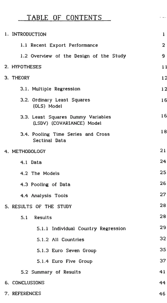
TABLE OF CONTENTS
1. INTRODUCTION
1.1 Recent Export Performance
1.2 Overview of the Design of the Study 2. HYPOTHESES
3. THEORY
3.1. Multiple Regression 3.2. Ordinary Least Squares
(OLS) Model
3.3. Least Squares Dummy Variables (LSDV) (COVARIANCE) Model 3.4. Pooling Time Series and Cross
Sectinal Data 4. METHODOLOGY 4.1 Data 4.2 The Models 4.3 Pooling of Data 4.4 Analysis Tools 5. RESULTS OF THE STUDY
5.1 Results
5.1.1 Individual Country Regression 5.1.2 All Countries
5.1.3 Euro Seven Croup 5.1.4 Euro Five Group 5.2 Summary of Results 6. CONCLUSIONS 7. REFERENCES 2 9 11
12
12 16 16 18 21 24 25 26 27 28 28 29 32 35 37 41 44 461
LIST OF FIGURES
1.1 World Foreign Trade
4 1.2 Foreign Trade of Developing Countries
4 1.3 Foreign Trade of European Economic
Community
5 1.4 Foreign Trade of OPEC Countries
5
1.5 Turkish Export and Import Values 8
5.1 Individual Country Results vs
Actual Export Values (All Countries] 31
5.2 Individual Country Results vs
Actual Export Values (Euro 5 Countries) 31
5.3 Results of All Countries Pooled
Against Actual Data Points (LSDV) 34
5.4 Results of All Countries Pooled
Against Actual Data Points (OLS) 34
5.5 Results of Euro 5 Group Against
Actual Data Points (OLS] 40
5.6 Results of Euro 5 Group Against
Actual Data Points (LSDV) 40
5.7 Results of Euro 5 group vs Actual
LIS T OF TABLES
1.1 World Foreign Trade
1.2 Turkish Export and Import Values 5.1 Individual Countries Regression Results 5.2 Regression Results For All Countries Pooled 5.3 Anova Table For All Countries Pooled
5.4 Regression Results For Euro 7 Group 5.5 Anova Table For Euro 7 Group
5.6 Regression Results for Euro 5 Group 5.7 Anova Table For Euro 5 Group
5.8 Summary of Regression Results
3 7 30 32 33 35 36 38 38 42
1.0 INTRODUCTION:
This study aims to construct a linear demand model for the Turkish export on the pooled time series and cross sectional data. Two regression models are utilized for this purpose in determining properness of pooling and the models are compared in terms of their fitness to the proposed application and their possible advantages in each different pooling arrangement. This study in essence does not aim to come to conclusions on the very complex mechanisms of Foreign Trade but attempts to make use of such data to show advantages and possibilities of pooling data and model selection for that pupose. Export data is used in this study on the basis of suitability of the characteristics of export data and export demand function for the above mentioned analysis.
This study is composed two phases, first phase was studying Turkish export characteristics and possible variables to be used to construct the export demand model. In that part of the study possible variables are included to the demand function however only the basic and theoretically most significant ones are kept for the analysis in order to simplify the model for the main purpose of this study.
At later phases the data is grouped in different arrangements in a progressive manner untill a sound and justified pooling arrangement is
achieved. Comparison of the models used is made at every step where a new pooling arrangement is examined.
A brief overview of the Turkish export trends and recent changes in foreign trade policies are presented in the following sections, in order to
familiarize ourselves with the environment where the data is actually generated and for reaching correct reasoning for the model required for the puroses of this study.
1.1 Recent Export Performance :
Export income is one of the most important sources of Income of the economy. It is even a more critical matter for the countries with large foreign trade deficits and therefore, it is essential that new markets be found to ensure its increase, that new undertakings be made, and that new incentives be provided. The importance of the export revenue has been well understood and aggressive actions toward expanding the export Income have been taken in the recent years.
Turkey's export income hcis showed a tendency to increase. The graph 1.5 depicts the changes in Turkish foreign trade trends. It can be observed that after 1980 a major change in the export trend takes place.
The factors that have effected demand to Turkish exports were
numerous. These variables that have impact on the export performance of a country, compose of wide spread factors from domestic politi- ical and economic decisions, to international trade and economic affairs. Changes on these factors will effect export performance of that country. Changes in the economic policy after 1980 had positive influence on the export performance of Turkish exporters. (I.T.O. 1986]
Among the various newly set regulations to activate foreign trade and to develop higher export performances, the industrialist groups find that incentives given to the export sector were the most fruitful in terms of progress achieved in that area (150,1987].
The Trade and Industry Associations shared the view that Turkish export performance showed a successful pattern in comparison to the world
conjuncture. The government estimate of 8.700 million dollar worth of 1986 exports have been actualized as 7.456 million dollar, which Is
Increased 61 In US dollars In 1981, 22 /. In 1982, 0.3 t decreased In 1983, and increased 24.5 7. in 1984, and 11,5 7 in 1985, contrary to the world trends. In table 1.1 a list of export and import constant dollar values are given for the last 25 year period.
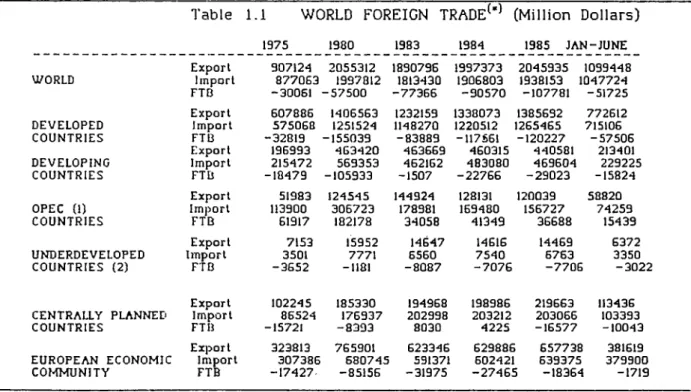
The world foreign trade values in different country groups are presented in table 1.1 . Comparing the export trends in those country groups' to Turkish export performance (table 1.2) it may be observed that between the period 1980 and 1983 the developed countries had 13 7 less exports, developing countries had approximately no change while Turkish exports had a 16 7 increase. Similarly increasing treads are observed between the 1984 and 1986 period. * (*)
Table 1.1 WORLD FOREIGN TRADE^'^ (Million Dollars)
1975 1980 1983 1984 1985 JAN-JUNE Export 907124 2055312 1890796 1997373 2045935 1099448 WORLD Import 877063 1997812 1813430 1906803 1938153 1047724 FTB -30061 -57500 -77366 -90570 -107781 -51725 Export 607886 1406563 1232159 1338073 1385692 772612 DEVELOPED Import 575068 1251524 1148270 1220512 ]1265465 715106 COUNTRIES FTB -32819 -155039 -83889 -117S61 -120227 -57506 Export 196993 463420 463669 460315 440581 213401 DEVELOPING Import 215472 569353 462162 483080 469604 229225 COUNTRIES FTB -18479 -105933 -1507 -22766 -29023 -15824 Export 51983 124545 144924 128131 120039 58820 OPEC (1) Import 113900 306723 178981 159480 156727 74259 COUNTRIES FTB 61917 182178 34058 41349 36688 15439 Export 7153 15952 14647 14616 14469 6372 UNDERDEVELOPED Import 3501 7771 6560 7540 6763 3350 COUNTRIES (2) FTB -3652 -1181 -8087 -7076 -7706 -3022 Export 102245 185330 194968 198986 219663 113436
CENTRALLY PLANNED Import 86524 176937 202998 203212 203066 103393
COUNTRIES FTB -15721 -8393 8030 4225 -16577 -10043
Export 323813 765901 623346 629886 657738 381619
EUROPEAN ECONOMIC Import 307386 680745 591371 602421 639375 379900
COf^MUNITY FTB -17427 -85156 -31975 -27465; -18364 -1719
(1) Algeria, Equator, Gabon, Indonesia, Iran, Irak, Kuwait, Libya, Nigeria,
Qatar, Saudi A rab ia, United Arab Em irates, V e n e z u e la
(2) Afghanistan, Bangladesh, Benin, Botswana, Burundi, Central Arab Republic,
Chad. Democratic Yemen, H abeshlstan, Gambia, Guinea H aiti, Lesotho, M a la w i Sudan, Som ali, Uganda, Tanzania, N ig e r, Upper V o lta
(*) Monthly S ta lls tic a l B u lle tin January 1987, United Nations.
GRAPH 1.3 EUROPEAN ECONOMIC COMMUNITY
if) •O onV-EXPORTS
WM^
BALANCE OF
1'RADE
1 9 7 5 1 9 8 0 1 9 8 3 1 9 8 4 1 9 8 5 1 9 8 5 (/) <n ^ h (55 D O sz-8
4 0 0 3 0 0 -200 -100-EXPORTS
GRAPH 1.4OPEC
(M illio n d o lla rs )
IMPORTS
M
BALANCE OFTRADE
W 1 9 7 5 1 9 0 0 1 9 8 3 1 9 8 4 1 9 8 5 1986(/)
O
8
2GRAPH 1.1 WORLD FOREIGN TRADE
(M illio n d o lla rs )
EXPORTS
IMPORTS
BALANCE OF
TRADE
1 9 7 5 1 9 8 0 1 9 8 3 1 9 8 4 1 9 8 5 1 9 8 5
GRAPH 1.2
WORLD
FOREIGN TRADE OF
DEVELOPING COUNTIES TO..
DEVLPED
D E V L P IN G R ^ OPEC
V777A
EUROPA
7 0 0 (/) I?) g o I-1 9 8 2 1 9 8 3 1 9 8 4 1 9 8 5
The decrease in export earnings in 1986 may be accounted for the decrease in raw petroleum prices, forcing especially Iran and Irak to lower their exports from Turkey. However this decrease is compensated, and in 1987, between the period January november Turkish exports reached to US $ 8,985.925, value which was a 20.5 % increase.
In the table 1.1, the trends in foreign trade for various
significant groups of countries are depicted. Also in the graphs 1.1 to 1.4 the changes in world trade are shown. In 1986 world trade has increased 13 /. and the world imports have a growth rate of over 10 Examining movements within the world trade, it is observed that majority of this activity is on the developed countries and not within the under developed or developing country groups. The OPEC countries had increased their imports only 2.6 7. while their exports have decreased 3.4 7.. Turkish exports, on the other hand, have been following the increasing trend recently. In the table 1.2 and from the graph 1.5 the changes in the
Turkish Exports and Imports are presented. A change in the rate of growth after the year 1980 is noticeable.
A brief survey of international trade is sufficient to see the
complexity of the issue. The increases and decreases are effected by many factors of which some are quite complex and some are not easy to identify.
Tablo 1.2
TURKISH EXPORT AND IHPORT VALUES
(1000 DOLLAR)
FOREIGN TRADE
YEARS
IMPORT
EXPORT
BALANCE
1963
687616
368086
319530
1964
537396
410771
126625
1965
571952
463738
108214
1966
718269
490507
227762
1967
684668
522334
162334
1968
763663
496419
267244
1969
801235
536833
264402
1970
947605
588476
359129
1971
1170841
676601
494240
1972
1562553
884968
677585
1973
2086214
1317082
769132
1974
3777558
1532181
2245377
1975
4738558
1401075
3337483
1976
5128646
1960214
3168432
1977
5796277
1753026
4043251
1978
4599024
2288162
2310862
1979
5069431
2261195
2808236
1980
7909364
2910121
4999243
1981
8933373
4702934
4230439
1982
8842481
5745973
3096508
1983
9235001
5727833
3507168
1984
10756922
7133603
3623319
1985
11343375
7958009
3385366
1986
11104770
7456724
3648046
T U R K IS H EXPO R T A N D IM PO R T V A LU E S
00 IMPORT VALUES YEARS Graph 1-5 EXPORT VALUES1,2 Overview to tlie Design o f the Study
:
The export demand function is a function where apart from the possible general variables like exchange rate, gross national product (GNP) etc, variations due to differences specific to each country and/or each period may become a statistically significant factor Influencing the demand function. Similarly, demand to the Turkish exports may be assumed to be governed by the factors common to all those general variables but at a rate significantly different for each country. The same argument is true for
time vise variances which may be quite complex for capturing by simple general variables. These changes among different countries and periods may
limit pooling of time series and cross sectional data unless proper model selection is achieved. Two independent variables are used in the analysis. These explanatory variables are the Gross National Product of countries studied and rate of Exchange between Turkish lira and the currency of the importing country. These variables are shortly referred as GNP and EXCH, in the following sections. In order to satisfy linearity these variables are used in the logarithmic form.
For this study a data set that had both time series and cross sectional variances, together with theoretically sound but reasonably simple
function were required. In that order, a 25 year time series and 10 country cross sectional data set for export values are utilized on two linear
regression models namely ordinary least squares COLS) and least squares dummy variables (LSDV) models .
The countries that are used in the analysis have been selected
according to their past import performance from Turkey. The data set contains the ten countries that have ranked as the top ten importers of Turkish goods. on'l V / M*-·' c i)i ^ S’' ·■ ■ s. i e. I. i Vi: V3 i ;“0 i: ■; t ·■': ;S • ^ : C i v y c o , ‘ i i i . . f c ' · : V . , I ' l U ' i ^'r· -Vi.'tr<VK’ViV’S' o!' crosr:: 10
2. HYPOTHESES:
The following hypotheses} have been defined for this study. In the following sections the validity of these hypotheses will be analyzed.
Hj! There exists a positive relationship between the Exports
from Turkey in the year t and GNP (Gross National Product) of the importing country in the year t.
In formulating this hypothesis, it is assumed that demand for exports from country P will increase by the growth of gross national
product of the importing country.
Hj: There is a positive relationship between the demand for Exports from Turkey in year t, and the Exchange rate between Turkish lira and the currency of the importing country in year t.
This hypothesis simply takes in to account the fact that cheaper the Exported goods get, higher quantity to be demanded. The export goods get more attractive as their price for the importer reduces.
H3: The LSDV model is a better estimator of the actual demand pattern to Turkish exports.
H4: The pooling of cross sectional and time series data is
appropriate method for the analysis of Export demand to Turkish goods.
3.0. THE THEORY;
This study makes use of a multiple regression analysis on pooled cross-section and time series data. The Study employs C ovariance
(LSDV) and OLS models. In the following sections, description and basics of multiple regression, models used and pooling of time series and cross section data, are presented.
3.1. Multiple Regression:
When the examined dependent variable has the posibility of dependence on more than one Independent variable, a multiple regression methodology is employed to estimate the model in order to offer explanations on partial effects of each variable in the equation. The use of the methodol
ogy enables the researcher to see the effect of changes in one variable while all others are held constant. A typical regression may take the fo l lowing form.
E (Y )u Oir
where;
Y : is the dependent variable
E(Y] ; is the expected value of the dependent variable ; is the constant term (the intercept)
: is the slope coefficient of independent variable Xj Xj : is the independent variable
£ : is the error tenn
This equation indicates that observed values differ from this equation by the error term e . The coefficients Pj are the partial
derivatives of the E(Y) with respect to Xj. Due to this property these coefficient are sometimes refered as partial regression
coefficients. The dependent variable Y is often called regressand and the right hand side variables are called regressors.
Multiple regression analysis measures the effect of a small
change in the independent variable Xj on Y while keeping effects of other variables constant. By this capability, the methodology differs from regressing Y on each Xj, and ignoring the effects of the other variables .
o o
The basic assumptions of the Least Squares analysis are,
the error terms have a mean of zero, the error terms have the same variance,
different error terms are statisticaly independent the error terms are normally distributed
and finally the right hand side variables are statistically independent of the error terms
The coefficients Pj and qj, are obtained by setting up
the equation to minimize the sum of squared error term. Taking par tial derivatives of this equation and equating them to zero yield the "normal equations". The procedure requires the means of all variables Xj, Y, the sum of squares and sum of products, in order to use
them in the calculations of the results of the above mentioned normal equations.
and
S ,j»2 X„.Y,ip‘ p n XjY
S yy P Y ^ - n ^ P .-.2
where,
i j = {1,2,3,...K> and K is total number of independent variables p - { 1 ,2,....n> and n is the total number of observations
then solving the simultaneous equations given by,
^ I*
for all i-{l,2,...K>
then the intercept term is obtained by simple arithmetics.
The residual sum of squares, which is reffered to as the unexplained part of the regression, is expressed as:
RSS . - Z P, S „ For all i
In search of a relation between the dependent and the Independent variables, basic test statistics are to be conducted. These basic statistics are t-statistics, F statistics . R“ value is also ob tained to see the power of regression. Briefly, by the use of t statistics the existence of a systematic relationship or in other words, test of whether a coefficient of a variable is statistically different from zero may be checked.
The F statistics on the other hand, Is advantageous in multiple regression where there are several independent variables, obviously testing R “ 0 cannot be justified with a tests on single coefficients since one would not know which coefficient to look at. The practical way to test R^=0 against R^>0 in the multiple regression model is the F test. F test checks the significance of all independent vari ables as a group. F test is a one tail test where the large values of' the computed F statistic would favor R^>0 against R^=0.
Coefflclant of multiple determination, measures the ex
planatory power of the regression equation the fraction of the varia tion in the observed values of Y that the estimated regression equation can account for. Simply:
RSS RGSS
TSS
2
- Y.)2 (Yt - T i where;
RSS: Residual Sum of Squares, RGSS: Regression Sum of Squares, TSS: Total Sum of squares.
The computer program employed In this study calculate the test statistics automatically.
3.2. OLS Model:
Both models used in this study are least squares models. The Ordinary Least Squares model, which the basic formulation is explained in the previous section, is the most simple and general form of the least squares model where the pooled cross section and time series data are analyized in the form given in the multiple regression section. It will provide a common intercept term, and partial regression coeffi cients for the independent variables. This model may be inadequate in cases where homogeneity of partial regression coefficient or in short slope homogeneity and/or Intercept homogeneity are in doubt. The above mentioned assumptions are valid for this model.
3.3. LSDV [Covariance] Model;
The Least Squares Dummy Variable model which is also called as covariance model, takes into consideration the class effects, that may result due to the factors specific to each class that are ignored
during formulation by any reason. This model may be used for the cases where the classes have common slopes, and different intercepts, or for classes that have different slopes but common intercept, and finally for classes which have different intercepts, different slopes. The
case where both slopes and intercepts are common will mean that OLS and LSDV are practically identical and both will yield the same result.
In this study the case where slopes are common and intercepts are different will be utilized since it is the case fits to the purposes of our study. The common slopes assumption will show pooling success and the intercept difference will indicate class effect and this will be a credit for use of dummy variables to capture this class effect.
Establishing the ecjuation for the LSDV model one must consider
the F test he wishes to carry out to test structural changes. In our study we shall only look in to the case where the slopes are common and the intercepts are free to differ from class to class (in this study each country is considered as a different class). The equation for this model, when used with a computer program that generates the intercept term automatically, and for cross sectional dummy variables- only, will be constructed as:
a
where,
and.
where,
Cjj: dummy variable that takes the value 1 or 0 is the intercept coefficient for dummy variable i, X: is the explanatory (Independent) variable,
p.· is the slope coefficient for variable X^, is the error term
i= {i,2 ,....P), t - { l , 2 .... M>, k-{2,3,....K}
P is the total number of cross sectional units, M is the total number of series units,
K is the number of Independent variables +1
An obvious question with regards to covariance model is whether the inclusion of the dummy variables and the consequent loss of the number of degrees of freedom is really necessary. The reasoning un derlying the covariance model is that in specifying the regression model we have failed to include relevant explanatory variables that do not change over time (and perhaps others that do change over time but have the same value for all cross-sectional units), and that the in
elusion of dummy variables Is a cover up of our Ignorance. If in
doubt, the need for the inclusion of the dummy variables may be Jus tified by means of F tests CKmenta.l 986]. To do this we need to es timate the regression equation with and without the dummy variables and compare the resulting error sums of squares by means of an F test. Similarly we are also cautious about the appropriateness of pooling of observations under the assumption of all cross-sectional units have common (same) slopes, again In that case we will estimate the regression coefficients for each cross-sectional unit and compare the error sums of squares with that obtained from the application of Least Square Dummy variables (LSDV) model, by the help of another F test.
3.4. P o o lin g o f Time se rie s and Cross Section Data
One major application of analysis of variance and covariance is in the problem of pooling cross-sectional and time-series data to decide on questions like whether or not to estimate the pooled regression with different degrees of pooling.
By pooling one may obtain a larger set of data and with a proper model will be able to estimate a single function instead of a number of
single equations.
In search of an answer to the questions mentioned above, hypothesis for each case are tested by means of a series of F tests.
For these tests Residual Sum of Squared errors, from OLS model RSSj, LSDV model RSS2 and finally the individual regression
RSSj's sum for the RSS3 are needed. These residuals and their con sequent degrees of freedoms are summarized below.
d.o.f
OLS MODEL RSS, mp-k LSDV MODEL Individual RSS2 mp-p-k+1 2 RSS,-s RSS3 2 (M,-KP) - p(m-k) Where;m; is the number of observations,
p: is the number of different classes and,
k; is the number of independent variables plus one.
A simple yet important indication of the above formulation of degrees of freedom is the fact that there is a limit to the number of dummy variables that can be introduced to the regression equation, for a given number of time series observations, variables and cross sectional units. Otherwise, the degrees of freedom may become negative, and calculations of F values will not be possible.
Basicaly there are three F tests to be conducted; 1. The F test for the hypothesis
differences of slopes between classes, will be as;
_ (RSS2-RSS3V(pk-p-k-H 1 ) "" CRSS3)/(ptin-k))
if the null hypothesis is rejected, this will Indicate that there is no slope homogeneity. This result will be accounted for poor pooling arrangement.
2. The F test for differences in intercepts Cconditional on slope homogeneity)
(RSSj-RSS^J/Cp-l) ~ CRSS2)/(pm -p-k+U)
Accepting the will be another evidence for propemess of pooling, However, rejecting H/.o may indicate that pooling is good, under LSDV model which will be the prefered model for this case.
3. the hypothesis for overall homogeneity of the relation as one regression Is,
and the related F test will be,
Fo =_ (RSS,-RSS3)/(kCp-D)(RSS3)/(p(m-k))
Rejecting alone may mean rejection of pooling. However, If Inter cept homogeneity is rejected while the slope homogeneity is accepted, the interpretation may be in favor of pooling provided that LSDV model is used to estimate the regression equation. Furthermore rejecting Hg will indicate denial of appropriateness of OLS model too.
To summarize, the F tests are used to test the properness of pooling and fitness of model. If the slope homogeneity is rejected the pooling arrangement is also rejected and intercept homogeneity will need not to be checked. One cannot credit any of the model in such case.
If slope homogeneity is satisfied then one need to check intercept homogeneity. If the Intercept homogeneity is also satisfied this will mean pooling was properly done and OLS is sufficient as a model. However if intercept homogeneity is rejected then pooling may or may
not be appropriate depending on the overall homogeneity. In that case one shall look to the overall homogeneity. If overall homogeneity is satisfied the pooling will be still appropriate and OLS will be
prefered against LSDV. However, if the overall homogeneity is rejected while slope homogeneity is satisfied this will be a result in favor of LSDV model and pooling will still be appropriate.
4. METHODOLOGY;
The hypotheses that have been established are tested
by using multiple regression analysis for 25 year time period and across ten countries. The ten countries, composed of USA, European and Middle East countries, which are listed below. These ten countries
accounted for the 63.13 X of the foreign trade volume and more significantly they were recipients of 68.41 X of our exports, in the year 1986 (Treasury and under secretary of Foreign Trade 1987 Summary output). These top Importers in the order according to their 1986
imports from Turkey, are:
o W. GERMANY o ITALY o IRAN o IRAK o U.S.A. o SAUDI ARABIA o ENGLAND o FRANCE o HOLLAND o BELGIUM-LUXEMBOURG
These ten countries are combined in different arrangements in order to obtain best pooling group.
In the initial stage of the study, the explanatory variables were tested for significance and each was considered as a potential for improvement of the regression equation. Some of these variables such as the Raw oil Prices, proved to be insignificant, whereas some were insufficient in data, and some had weak theoretical backing. An
evaluation process took place in the course of selecting the proper variables for the regression analysis. Variables that have been tried
in the equation during the initial stage were :
о DGNP Change in Gnp between t-^1 and period.
□ ВОТ The balance of country's exports and imports. □ PETR Petroleum prices (constant for all countries)
□ IMP Imports that Turkey has made to the-. P^^ country. □ PREVEX Previous exports tp the P^^ country
□ GNP Gross -National· Product of importing country
□ EXCH rate of Exchange between Turkhlsh lira and the currency of the importing country.
The GNP variable is introduced to the equation assuming that countries having higher GNP values may have more resources (money) to spend on imported goods and that they would prefer to import from other countries. Therefore a positive, relation is assumed for this variable. Similarly the DGNP variable is introduced to see if the change in GNP value better express the demand to Exports than the simple GNP value. However this variable during the study came out to be less significant and no additional improvement achieved by intro ducing this variable in to the equation.
The ВОТ the balance of trade variable was introduced assuming that countries that import more goods to Turkey would tent to export more from Turkey. However this variable did not improved the equation as expected.
Petroleum prices v/ere considered as a variable since especially for the petroleum producing Arab countries its increase would suggest
more resources to import goods from other countries on of which was Turkey. However, its increase and decrease also meant increase and decrease of GNP of those countries. This raised the problem of multlcollinearity, which is the problem encountered with variables that one of which is a linear combinations of the other.
The variable PREX was considered on the assumtion that a ”Leaming by Doing" mechanism exists and improves export performance. Although
this assumption would come out to be significant. Its quite high correlation with the export values, caused its elimination from the function.
In aggregate studies as this study, certain level of correlation among the explanatory variables is inevitable. Keeping many variables that are correlated with each other would only complicate the matter rather than to explain it better. Finally, lesser but useful right
hand side variables are utilized considering the main purpose of this study.
Discarding these variables but the Gnp and Exch, of course
in no way suggests that they may be meaningless in any other form under a different method of analysis, nor does it invalidate any
other study that have used such variables in the above mentioned form.
To summarize, the selected variables are the variable GNP which
is the Gross National Product of importing country, and the EXCH which is the Exchange rate between Turkish lira and currency of the import ing country.
4.1. Data:
Data on the Export values in dollars have been obtained from the Prime Ministry, Treasury and Foreign Trade Under Secretary.
Data Collection and Processing Department. The documents (the computer outputs of Turkish foreign trade values sorted country wise, in terms of country groups like OPEC, EEC etc.) contained the export figures for all countries, country groups, continents etc. together with the import figures, percentages and performance orders.
The data on the Gross National Product and Exchange rate, are obtained from the International Financial Statistics of the International Monetary Found. The GNP values are Indexed values of the US dollar amounts, and the Exchange rates are calculated by converting exchange rates In currency per Turkish Lira (e.l. 1 DM=12 TL). The exchange rates are the period averages of each year.
4.2. The Model:
There are two different models In this study. The first Is the
Ordinary Least Squares model. Given P countries and M observations on the variables, the OLS model for the ten country is set up as :
log(EXP)j = OfQ+Pjlog(GNP)jj+P^Log(EXCH)jj+e,^
where 1={1,2,3,..,.P>: and t= { 1,2,3... M), for P countries and M years
are the regression parameters, is the error term.
Since a linear multiple regression analysis Is adopted In this study the independent variables and the dependent variables are arranged in logarithmic form. By this the linearity assumption Is satisfied.
F tests are conducted In order to test the overall significance of the
regression equation exhibited above. In order to test the significance of individual regression coefficients t tests are carried out. All t tests are one-tall tests with the null hypotheses of, ^^=0 for all 1= {1 ,2 }; and the alternative hypotheses of ^^>0, since the expected relationship between the variables on the right side of equation and the left are
positive. This model is employed for the three pooling groups to be defined in the next section.
The second model is the Least Squares Dummy variable model (LSDV)
which is also called Covariance model. The model utilizes P-1 dummy vari ables for the P countries pooled, in order to better estimate the effect arising from country differences. The LSDV model by definition has no com mon intercept term, this characteristic of the model may arise problems if
the computer program utilized calculates Intercept term automatically.
Having P-1 dummies enables one to overcome the problem of automatic inter cept calculation of the statistical program. Then the term in the
equation is the first country’s intercept term.
The LSDV model is then take the form,
I
obCEXP), . a„*a,C„,,*..*Oi(p_„C„,(p.„*ptog(GNP)„*p^Log(EXCH)„.£
where;
is the country dummy variable (1 or 0) the intercept term for country i
P: is the slope coefficent is the error term
In the most general form, including dummy variables to capture both time variance and cross sectional variance is possible however includ ing these dummy variables induce loss of degrees of freedom. In this study although initially dummy variables were included for both time and cross sectional variance, time dummy variables are dropped due to calculation limitations for F tests with reduced degrees of freedom. Therefore only country dummy variables are used in this study.
4.3. P o o lin g o f data:
As it was referred to in previous sections this study utilizes
pooled time series-cross sectional data. The virtue of this approach comes from the enlargement of the sample size considerably. As a result, a single pooled regression that has the superiority of
accommodating higher precision than a number of different regression. However the pooling, if done inappropriately, has the risk of intro ducing aggregation bias which may result in erroneous estimates. In
our study the tests mentioned on the Theory section are conducted to test the appropriateness of pooling T/avas and Vardlabasls.l 987).
In order to test the appropriateness of pooling, first the usual t and the F tests are conducted. Secondly, covariance analysis is employed to test the structural changes over the different pooling groups. The study contains three different pooling arrangements. First arrangement is the pool composed of all ten countries, second, is the seven European countries (including USA) of the initial set excluding Iran, Irak, Saudi Arabia, third is the five countries selected after examining results of the above two and the individual country
regressions. F tests that have been formulated in the theory section are employed in conjunction with the analysis of variance procedures.
4.4
A n a ly sis T o o ls :
In this study the Statistical Package for Social Sciences, (SPSS) Personal Computer version has been utilized to analyze the data. For data preparation and calculations computer prograins such as Lotus and Eureka have been employed to assist the analysis.
The SPSS program is utilized for selection of significant variables at the first stage. The program it self tests and selects each variable proposed according to their T values. The variables that do not con tribute to the equation are eliminated from the equation. Forward and
Backward selection routines are used for this purpose.
5. RESULTS OF THE STUDY:
The results of the multiple regression analysis, on different pooling arrangements for the cross sectional units are presented in this section. The order of presentation of results are as follows.
First, the results of multiple regression of individual countries which will be needed for the calculation of F values are presented. Following the individual regressions, the results of the pooled regression of time series and cross sectional data for all ten countries are given. Thirdly depicted are the findings of the pooling arrangement of seven countries excluding Iran, Irak, Saudla Arabia. This arrangement is named as EURO 7 however, this group
contained USA data. The last results belong to the arrangement which is the subset of previous group Euro 7, and it consists of Germany, Italy, England, France, Holland, this grouping is constructed after
observing the results of the other regression and F tests as well as individual regression results. This last group have been labled as
EURO 5.
The form of the regression equation is same for all pooling
arrangements with only difference in the number of cross section dummy variables. The number of country dummy variables are one less of the number of countries involved In that arrangement for each run. The number of time series observations (m), nuber of counries included for that trial (p) and finally number of Independent variables plus 1 (k)
is given on the Anova tables together with the residual sum of squares, degress of freedom and mean square values.
The results of each different pooling arrangement Is also presented in a grafical presentation. For the construction of these graphs
actual export values used In the study are plotted against each other on both axis. This, as expected formed the 45° line representing the actualization level. The values obtained from the estimated demand function of each trial, corresponding to the actual export values are ploted against to these. Closer the model estimated values positioned against the 45° line the better the regression shall be.
5.1,1. Individual Country R e g re ssio n :
Each country that has been used for this study is initially studied individually. Multiple regression results are obtained for each
country alone. These results were required for evaluating validity of the proposed relations for each country used in the study and for obtaining the individual residual sum of squares to be used in the calculations of F tests summarized in previous sections. The
results of these regression runs are depicted in the table 5.1.. As these results will be common to all other analysis they will not appear on the regression results of above mentioned pooling arrangements.
All of the individual regression have high adjusted R" and
significant F values. The estimated coefficients are comparable in their magnitudes and exhibited signs are in agreement with the hypotheses . Having these results provided necessary conditions for continuing with the analysis and use the results of individual
regressions in the analysis for the pooled cases.
The coefficient pj Indicate that one unit Increase in log
GNP would increase Log of Export value by 2.915 for Germany while keeping the variable log EXCH constant. Similarly a 0.3415 unit in crease in log export value will be expected for a unit increase in log exchange rate.
Graphs 5.1 and 5.2 depicts the values obtained from individual regression equation for each country against the actual export values for that country. In the graph 5.1 values obtained from all ten counrtry are plotted. In the graph 5.2 only the values from EURO 5 arrangement are plotted in order to be able to compared the results with the results of EURO 5 when the data is pooled (graphs 5.5 and 5.6) The distribution of points along the solid line (which is a 45 degree line) indicates how well the regression has explained the actual varia tion of the data in a different way.
Table 5.1, Individual Regression Results
Individual R e gre ssio n A n a ly sis
Country ''o Const Pi Log Gnp ^2 Log Exch Adj. R^ F GERMANY -0.4627 (0.618) 2.9151 (0.341) 0.3109 (0.041) 0.974 458.17 ITALY 1.1921 (0.960) (0.453)2.3850 0.4870 (0.087) 0.911 123.73 IRAN -2.2784 (1.641) (0.809)3.5271 (0.235)0.9557 0.802 49.75 IRAK -4.8093 (1.218) 4.6165 (0.892) 0.4422 (0.254) 0.850 69.01 U.S.A. 2.6915 (0.933) 1.0179 (0.529) 0.3197 (0.070) 0.855 71.99 SAUDI A. -1.7852 (0.333) 2.6839 (0.226) 0.9532 (0.086) 0.965 677.89 ENGLAND -0.4756 (1.315) (0.729)2.4113 0.3882(0.076) 0.867 79.27 FRANCE 0.2379 (0.4 1 5) 2.3164 (0.232) (0.043)0.2897 0.968 362.87 HOLLAND -0.9977 (1.441) (0.303)2.8107 0.2767(0.052) 0.979 563.69 BELG-LUX. 1.6139 (0.823) 1.6254 (0.614) 0.3536 (0.078) 0.886 94.48
Standarl Errors in Parenthesis
? l·-< Q _) < D o <
g
a: u. a X m O) oINDIVIDUAL COUNTRY RESULTS
AGAINST THE ACTUAL EXPORT VA1..UES
_L .U: -1 1:,. 4--f-/■^+1- +i - b Y ^ - i '- i' 1 + + + 1 2 3 4 5 6
Log EXP (FROM REGRESSION) The regression line has the form y=0.97A(x)+0.108
+ ALL COUNTRIES < I-< Q 3 1 -u <
o
n: LL o> OINDIVIDUAL COUNTRY RESULTS
AGAINST THE ACTUAL EXPORT VALUE
3.80 4.32 4.84 5.36 5.88
Log EXP (FROM REGRESSION) The regression line has the form y=0.999(x)+0.0005
-I- EURO 5 COUNTRIES
5.1.2. A ll Countries :
The first pooling arrangement has the combination of all ten countries where 25 by 10 data points are Included in the analysis.
The regression results obtained are presented in table 5.2..
Table 5.2, Regression Results for All Countries
A ll
Countries
Model “ c Const Log Gnp h Log Exch Adj r2 F OLS -4.1159 (0.377) (0.20 1)4.6327 (0.026)0.1050 0.720 321.95 LSDV 3.8107 (0.215) 0.3282(0.047) 0.863 144.16Standard errors are in the parenthesis
The coefficients Pj and ^^e the marginal contributions of
the Independent variables Log Gnp and Log Exch. When the data for all ten countries are pooled the values came out to be 0.72 for OLS and
0.86 for LSDV which Is rather an Indication of a weak regression.
The regression results for both OLS and LSDV (Covariance) model find the Exchange variable and the Gnp as significant. At the same time, one might note the improvement in the adjusted values, going from OLS to LSDV model. However, a slight reduction in the significance level for
2 the beta coefficients is observed in return for this increase in R .
Constructing the analysis of variance table 5.3, we get the following residual sums of squares:
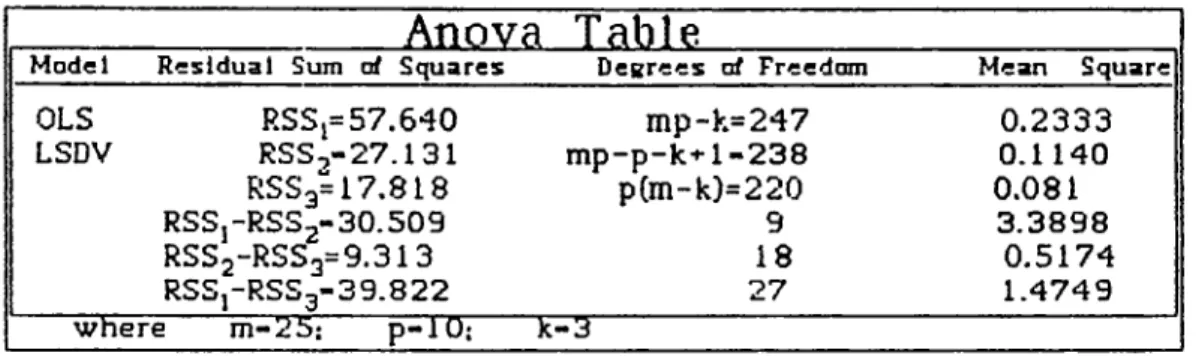
Table 5.3, Analysis of Variance table for All Coiantries Pooled
Anova T able
Model Residual Sum erf Squares Degrees of Freedom Mean Square
OLS RSSp57.640 mp-k=247 0.2333 LSDV RSS,-27.131 mp-p-k·*· 1-238 0.1140 RSSg=17,818 p(m-k)=220 0.081 RSSj-RSS2“ 30.509 RSS2-RSSg=9.313 9 3.3898 18 0.5174 RSS,-RSS3-39.822 27 1.4749 where m-25; p-10; k-3
The F tests conducted by utilizing the calculated values are: a) For slope homogeneity,
F*2 - (0.5174/0.08U - 6.387 and the F critical value from the F distribution tables is, Qggd 8,220) - 2.03, since the F
critical value is less than F calculated, we reject the hypothesis
that the slopes are common for all countries at the 99 7, level. This result suggests that pooling is not so appropriate when all ten countries are pooled together.
It is trivial to calculate the Fj value after rejecting the slope
homogeneity since the Fj test is a conditional test that requires common regression slopes.
b) The test for overall homogeneity is,
F*3=18-21 and the F^ ogg(27,220) = 1.79
Since, F*g is larger than F^ the overall homogeneity hypothesis is
also rejected. Therefore proposed pooling arrangement is not appropriate.
RESULTS OF ALL COUNTRIES POOLED
ACTUAL DATA AGAINST MODEL
I— q: o Q. X Id H q: o Cl y bJ Di 0
RESULTS OF ALL COUNTRIES POOLED
ACTUAL DATA AGAINST MODEL
Log laPOkT
The regression coefficients obtained from both models are used to
build the regression equations for OLS and LSDV models. The actual data points against the model results are depicted for two models in graphs (5.3) and (5.4).
The 45° line in the graphs formed by entering actual Export (log) values for both axis and ploting the model values against them. The closer the points to the line the better the model fitts to the actual data (a dif ferent presentation of the value). As observed from the graphs,
although the pooling in the analysis found out to be poor, still the LSDV model has a better fit to the actual data than the OLS model.
5.1,3. Euro Seven :
Pooling the data in different country groups is as discussed in the pre vious sections, is a progressive procedure. One need to try many different combinations in order to justify pooling of time series and cross sectional data. At this stage the analysis will be carried out on the seven European countries, that were explained in the methodology section. The results of the regression analysis are summarized below.
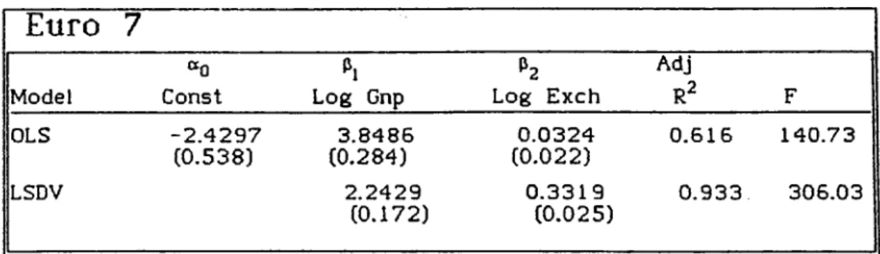
Table 5.4, Regression results of Euro 7 group.
Euro
7
Model
«0
Const Log Gnp Log Exch
Adj r2 F OLS -2.4297 (0.538) 3.8486 (0.284) 0.0324 (0.0 22) 0.516 140.73 LSDV 2.2429 (0.172) 0.3319 (0.025) 0.933 305.03
Standard errors are in the p aren th esis
The regression analysis for the OLS model calculated t values for Ex change rate variable as 1.437 and found it to be significant only at 15 % level. Whereas, the Gnp variable had 13.535 as t value and found out to be quite significant. On the other hand for the LSDV model calculated t value for the Exchange variable as 13.1 and found it as significant also together with the Gnp variable.
It is also important to note that there has been a substantial in crease in the adjusted value for LSDV as 0.933 compared to the value obtained in the previous case of 0.853 and a decrease in the of the OLS model from 0.72 of previous case's to 0.615. This result is in favor of the LSDV model over the OLS.
From the residual sum of squares obtained and presented in the table 5.5, relevant F values are calculated for each homogeneity verification.
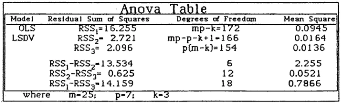
Table 5.5, Analysis of Variance table for EURO 7 group.
Anova T able
Model R esidual Sum of Squares D eg re e s of Freedom Mean Square
OES“ RSSj= 16.255 RSSj- 2.721 mp-k= 172 0.0945 LSDV m p-p-k+1-165 0.0164 RSS3= 2.095 p(m-k]=154 0.0136 RSSj-RSSj-13.534 RSS2~RSS3= 0.625 5 2.255 12 0.0521 RSSJ-RSS3- I 4 . I 59 18 0.7855 where m-25; p-7; k- 3
The F values calculated are compared with the table F^. Ccritlcal F values] values.
F*2 = 3.83 > ggg(12,154) = 2.3 and therefore
the hypothesis of common slopes are again rejected. Rejection of the common slopes hypothesis indicate that each country in the pooling group have significantly different trends in terms of the Independent variables gnp and exch. Therefore proposed pooling arrangement is inappropriate and a new grouping is necessary. Although this pooling combination have not
yielded the desired outcome, a significant improvement on the Fj value is achieved. This improved Fj value is an encouragment for further trials.
Finally, the F’ g = 60.51 value is obtained for the required test of overall homogeneity and compared with the F^ QggCl8,154J =1.87. The overall homogeneity is therefore rejected. Rejection of overall homogeneity suggests that pooling was indeed inappropriate.
5.2.4 Euro five Croup:
Another arrangement is made for the pooling of time series and
cross sectional data. The five European countries, have been selected out of the Euro 7 group with respect to their slope coefficients and
R^ values estimated from individual regression analysis. The countries Included in this group are Germany, Italy. England, France, and Holland. On the basis of these and studying the results of the previous pooling arrangements the Euro five group is established as the third arran gement.
The table 5.6 exhibits the regression results for this run.
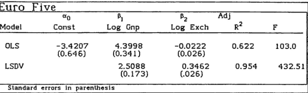
Table 5.6, Regression results of Euro 5 group.Euro Five
Model“0
ConstPi
Log Gnp h Log Exch Adj R^ F OLS -3.4207 4.3998 - 0.0222 0.622 103.0 (0.646) (0.341) (0.026) LSDV 2.5088 0.3462 0.954 432.51 (0.173) (.026)Standard errors In paren th esis
The regression results suggest that LSDV model Is a better fitting model than OLS . Obviously the has increased from 0.6 to 0.95 in LSDV model, and secondly the Exchange variable that had been insignificant in the OLS model with a negative slope coefficient of - 0.022 and t sig nificance at 40 X level, had also become significant and had positive
slope coefficient of 0.346, in the LSDV model. These findings provided support to the LSDV model as It also agreed with the theoretical expectations.
Table 5.7, Analysis of variance table for Euro 5 group.
Anova T able
Model R esidual Sum of Squares D e g re e s of Freedom Mean Square
OLS RSS,-12.972 RSS,= 1.452 m p-k=l22 0.1018 LSDV m p -p -k + l= l18 0.0123 RSS“3= 1.245 p(m-k)=l 10 0.0113 RSSj-RSS2= 11.52 RSS2-RSS3- 0.207 4 2.88 8 0.0258 RSS,-RSSa= 11.727 12 0.9772 where m=25; p=5; =3
38
The F values are then calculated to test related homogeneity hypothesis
f 2 — 2.28 < o_gg(8,110) =2.59
thus the hypothesis of common slopes is accepted. Accepting the hypothesis of homogeneous slopes brings the question of intercept homogeneity which is a conditional test on slope homogeneity. Fj value will be calculated to see if the intercepts are sig nificantly different from each other for different countries.
F*j =234.1 > F*Qgg(4,118) = 3.51 hence the common
Intercepts hypothesis is rejected. Rejecting homogeneous Intercepts hypothesis will indicate that there are indeed significant differences
b e t w e e n t h e i n t e r c e p t s o f e a c h c o u n t r y r e g r e s s i o n w h i l e t h e i r s l o p e c o e f
ficients are significantly homogeneous.
Last test for overall homogeneity will be done by calculating the
f *3 value,
Fg = 86.47 > F^Q9g(12.110) = 2.36,
this result rejects overall homogeneity hypothesis, indicating that there is no overall homogeneity. This result was actually an expected result since we already know that there is no intercept homogeneity. However, since we could established common slopes and see that there is indeed significant Intercept (class) effect, it is possible to talk about Just ness of pooling and make comparison between the two models.
ORDINARY LEAST SQUARES RESULTS
ACTUAL DATA AGAUJST MODEL
LEAST SQUARES DUMMY VARIABLES RESULTS
ACTUAL DATA AGAINST MODEL
The graph (5.4) and (5.5) given, presents the results in a graphical format. The graphical presentation may also be used to compare the results obtained from OLS and LSDV models. The distribution of estimated values around the 45° line indicate the closeness of the regression function to the actual demand. The closer the calculated values are the better their estimation power thus the better the model fitness.
The above results suggest that a LSDV is a better model for the pooled time series and cross sectional data and furthermore pooling in this form used with the LSDV model, is an appropriate arrangement.
5-3 Summary o f Results t
The individual regression runs depicted in the table 5.1 showed that, the hypothesized relationship is valid. The coefficients obtained from different regressions are comparable in their mag
nitudes and signs of coefficients were in agreement with the
hypothesized relation. The proposed positive relations seem to hold for individual cases as well as pooled cases.
A fter trying different pooling groups and variables, the above ex hibited results have been obtained. In short we have conducted regres sion analysis over three different arrangements for pooling time
series and cross section data. In the final grouping a desired and proper pooling arrangement have been achieved.
Results obtained for different pooling groups for the OLS and LSDV models are summarized in the table 5.8 It must be noted that for the LSDV model no constant term is depicted. This model utilizes different in tercept terms for each country to accomodate the country effects in con trast to the OLS model. F values obtained (the smallest F value being 26 for 25 observations and 2 degrees of freedom) are quite larger than the critical values thus this also indicate that the independent variables taken as a set are significant.
The export values obtained in the section 5.1.1 from the individual regres
S i o n equations of the 5 countries were plotted against actual data points
(actual export values) on graph 5.2., and the values obtained from the
single regression equation of the LSDV model for the EURO 5 countries are also plotted in graph 5.7. against actual data point and printed for
comparison on the next page. The solid line in these two graphs are fitted by an other regression and the coefficients calculated are shown on these graphs. Examining these equations, one would see that both are the equation of the 45 degree line. In simple terms, by utilizing pooled data and LSDV model it is possible to obtain a higher precision in a single equation then what one may obtain from a set of equations regressed for that same group
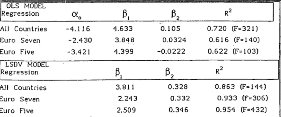
Table 5.8., Stunmary of Regression Results
OLS MODEL Regression «0 p, Pz R^ All Countries -4.116 4.633 0.105 0.720 (F=321) Euro Seven -2.430 3.848 0.0324 0.G16 (F-140) Euro Five -3.421 4.399 -0.0222 0.622 (F=103) LSDV MODEL Regression p. p. R^ All Countries 3.811 0.328 0.863 (F=144) Euro Seven 2.243 0.332 0.933 (F=306) Euro Five 2.509 0.346 0.954 (F=432) k l
< < O D f-Ü < 0 1 Q. X IJJ 6
Analyzing the overall picture, one would see that for the OLS
model the explanatory power of the regression expressed by the
decreases as the of the LSDV model increases when better pooling arrangements are utilized. Secondly, the F values for both models are far above the critical values thus the set of variables used together are significant.
EURO 5 LSDV MODEL RESULTS
AGAINST TI--IE ACTUAL EXPORT VA1..UES
6.^0 5.B8 5.35 4 . 8 4 4 .32 -1- :l* -K -1; 7 1 -+ . -1-fX-|i ___ ■·* L - -H-_______ ?m O 5 LSDV MODEL 3 .8 0 4.32 4.84 5.36 5.88 6.40
Log EXP (FROM REGRESSION)
The regression line has the form y=0.9995(x)+0.002A .
G r a p h 5 , 7
Obviously the pooled case has the advantage of explaining the relation with a single equation whereas the results of individual regressions are obtained from different equations obtained for each country
individualy.