Frictional and vibrational properties of nanostructures

FRICTIONAL AND VIBRATIONAL

PROPERTIES OF NANOSTRUCTURES

a dissertation submitted to

materials science and nanotechnology program

of the Graduate School of engineering and science

of bilkent university

in partial fulfillment of the requirements

for the degree of

doctor of philosophy

By

Seymur Cahangirov

April, 2012

I certify that I have read this thesis and that in my opinion it is fully adequate, in scope and in quality, as a dissertation for the degree of doctor of philosophy.

Prof. Dr. Salim C¸ ıracı (Advisor)

I certify that I have read this thesis and that in my opinion it is fully adequate, in scope and in quality, as a dissertation for the degree of doctor of philosophy.

Prof. Dr. Atilla Er¸celebi

I certify that I have read this thesis and that in my opinion it is fully adequate, in scope and in quality, as a dissertation for the degree of doctor of philosophy.

Assoc. Prof. Dr. ¨Ozg¨ur Oktel

I certify that I have read this thesis and that in my opinion it is fully adequate, in scope and in quality, as a dissertation for the degree of doctor of philosophy.

Prof. Dr. Macit ¨Ozenba¸s

I certify that I have read this thesis and that in my opinion it is fully adequate, in scope and in quality, as a dissertation for the degree of doctor of philosophy.

Assoc. Prof. Dr. Mehmet Bayındır

Approved for the Graduate School of Engineering and Science:

Prof. Dr. Levent Onural Director of the Graduate School

ABSTRACT

FRICTIONAL AND VIBRATIONAL PROPERTIES OF

NANOSTRUCTURES

Seymur Cahangirov

Ph.D.in Materials Science and Nanotechnology Program Supervisor: Prof. Dr. Salim C¸ ıracı

April, 2012

Frictional and vibrational properties of low-dimensional nanostructures have been investigated using the state-of-the-art ab-initio calculations.

Stringent test of stability based on calculation of phonon dispersions have been performed for various materials having important potential applications in nanoscience and nanotechnology. Silicene, a counterpart of graphene composed of silicon atoms, is one of such materials with its suitability to well established sil-icon technology together with eccentric electronic structure due to its honeycomb symmetry. Vibrational spectrum of silicene is found to be exempt from imaginary frequencies upon the puckering of atoms in adjacent sublattices while preserving the symmetry necessary for occurrence of massless Dirac Fermions. Analyses of vibrational properties of silicene nanoribbons and carbon atomic chains revealed new interesting physics like fourth acoustical mode and long-ranged interactions due to Friedel oscillations.

Basic concepts of friction science like dissipation phenomena, adiabatic and sudden processes together with several simple models of friction have been sum-marized. A new method for calculation of corrugation potential between layered lubricants under constant loading pressure is introduced. Transition from stick-slip to continuous sliding regime is quantified through definition of frictional figure of merit for layered lubricants. Using this measure tungsten oxide is proposed as an oxidation resistant material which can outperform molybdenum disulfide as a superlubricant. It was found that, the corrugation strengths of graphene layers sandwiched between Ni slabs decrease as the number of layers increase.

Keywords: phonon, stability, silicene, friction, dissipation, sudden process.

¨

OZET

NANOMALZEMELER˙IN S ¨

URT ¨

UNME VE

T˙ITRES

¸ ˙IMSEL ¨

OZELL˙IKLER˙I

Seymur Cahangirov

Malzeme Bilimi ve Nanoteknoloji, Ph.D. Tez Y¨oneticisi: Prof. Dr. Salim C¸ ıracı

Nisan, 2012

D¨u¸s¨uk boyutlu nanomalzemelerin s¨urt¨unme ve titre¸simsel ¨ozellikleri ilk prensi-plere dayanan en geli¸smi¸s hesaplama y¨ontemleriyle incelendi.

Fonon eˇgrilerinin hesaplanmasıyla nanobilim ve nanoteknolojide ¨onemli uygulama potansiyeli ta¸sıyan malzemelerin kararlılıkları test edildi. Bunlardan birisi grafin’in silisyum atomlarından olu¸san analoˇgu olan silisen’dir. Silisen, g¨un¨um¨uz¨un silikon teknolojisine uyumunun yanında, sahip olduˇgu eksantrik elektronik yapısıyla da ¨onem ta¸sımaktadır. Silisen’deki atomlar yukarı ve a¸saˇgı hareket ederek titre¸simsel spektrumu sanal frekanslardan arındırmakta ve bununla birlikte k¨utlesiz Dirac Fermiyon’larının olu¸sumu i¸cin gerekli olan simetriyi korumaktadır. Silisen nano¸seritlerin ve atomik karbon zincirlerin titre¸simsel ¨ozelliklerinin incelenmesi sonucu d¨ord¨unc¨u akustik mod ve Friedel salınımlarından kaynaklı uzun mesafeli etkile¸sim gibi yeni fiziksel olgular ortaya konmu¸stur.

S¨urt¨unme biliminin temel kavramları olan enerji yayımı, adiyabatik ve ani olgularla birlikte s¨urt¨unmenin anla¸sılması i¸cin kullanılan birka¸c basit model ¨

ozetlenmi¸stir. Katmanlı yaˇglama malzemelerinin sabit basın¸c altında korugasyon potansiyelinin hesaplanması i¸cin yeni bir y¨ontem geli¸stirilmi¸stir. Bu malzemelerin yapı¸sma-kayma rejiminden d¨uzenli kayma rejimine ge¸ci¸si s¨urt¨unmesel ba¸sarım katsayısının tanımlanmasıyla kantitatif hale getirilmi¸stir. Bu ¨ol¸c¨ut kullanılarak, oksitlenmeye dayanıklı olan tungsten oksit malzemesinin s¨uperyaˇglama malzemesi olarak molibden disulfat malzemesinden daha y¨uksek performans g¨osterebileceˇgi ¨

one s¨ur¨ulm¨u¸st¨ur. Nikel y¨uzeyleri arasına konulan grafin tabakaların s¨urt¨unmeyi d¨u¸s¨urd¨uˇg¨u ve bu etkinin tabaka sayısıyla birlikte arttıˇgı g¨ozlemlenmi¸stir.

Anahtar s¨ozc¨ukler : fonon, kararlılık, silisen, s¨urt¨unme, enerji yayımı, ani olgular. v

Acknowledgement

I am inexpressibly grateful to my supervisor Prof. Salim C¸ ıracı for his guidance and support during my masters and doctorate studies. His foresighted vision always boosted the impact of our work by orders of magnitude. I feel proud for being a member of his condensed matter school which stands on a nearly half century experience of intensive research.

I would like to thank my instructors Prof. Cemal Yalabık, Assoc. Prof. ¨Ozg¨ur Oktel, Assoc. Prof. Mehmet Bayındır and Assoc. Prof. ¨Omer Ilday for their perfect teaching and for being outstanding examples as scientists. In particular I would like to acknowledge fruitful discussions with Prof. Cemal Yalabık and Assoc. Prof. ¨Ozg¨ur Oktel which were very helpful in development of this thesis. I would like to thank visiting instructors Prof. Chin-Yao Fong and Prof. Rolf Gerhardts for teaching us so much in a very short time.

I would like to thank Dr. Engin Durgun, Dr. Haldun Sevin¸cli, Dr. Ethem Akt¨urk and Dr. Hakan G¨urel for their close guidance during their presence in the group. I am sincerely grateful to my groupmates Mehmet Topsakal, Can Ataca, Hasan S¸ahin and Ongun ¨Oz¸celik for their friendship and outstanding collabora-tions. This thesis would certainly be lifeless without their colorful contribucollabora-tions.

I am grateful for the privilege of meeting Dr. Mecit Yaman who rejuvenated my mind. I would like to thank all members of UNAM family for providing a multidisciplinary research atmosphere and for joyful friendships.

I would like to thank my mother, father, sister, brother and my best friend Esat C¸ etin Musabeyli for always being there for me.

This thesis is dedicated to my beloved wife Naide. There is no way to thank her for the love and care she has provided all these years for me and our little bundle of joy, Alim.

Contents

1 Introduction 1

1.1 Density Functional Theory . . . 2

1.2 The Rise of Graphene . . . 6

1.3 The Renaissance of Friction . . . 8

1.4 Organization of the Thesis . . . 11

2 Phonons and Stability 12 2.1 Introduction . . . 12

2.2 Dynamical Matrix Formulation . . . 13

2.3 Small Displacement Method . . . 14

2.4 Stability of Silicene . . . 15

2.5 Fourth Acoustic Mode in Nanoribbons . . . 23

2.6 Friedel Oscillations in Carbon Chains . . . 28

3 Dissipation Phenomena 35 3.1 Introduction . . . 35

CONTENTS viii

3.2 Phononic Dissipation . . . 36

3.3 Electronic Dissipation . . . 38

3.4 Adiabatic and Sudden Processes . . . 40

4 Simple Models of Friction 42 4.1 Prandtl-Tomlinson Model . . . 42

4.2 Frenkel-Kontorova-Tomlinson Model . . . 46

4.3 Multichain Frenkel-Kontorova Model . . . 48

5 Frictional Figure of Merit 51 5.1 Motivation . . . 51

5.2 Layered Superlubricants . . . 53

5.3 Methods . . . 54

5.4 Critical Curvature . . . 55

5.5 Intrinsic Stiffness . . . 59

5.6 Frictional Figure of Merit . . . 61

5.7 Stick-Slip in Silicane: A Counter Example . . . 61

5.8 Discussions . . . 62

6 Superlubricant Graphene Layers 64 6.1 Motivation . . . 64

CONTENTS ix

6.3 Methods . . . 68

6.4 Adhesion Hysteresis . . . 68

6.5 Trends and Discussions . . . 70

List of Figures

1.1 Born-Oppenheimer and Self-Consistent Field Approximations. . . 3

1.2 The scheme for self-consistent DFT calculation. . . 4

1.3 General dependence of friction regimes on sliding velocity and ratio of stiffness to the corrugation potential. In the drag regime, friction force is proportional to velocity while in the superkinetic regime it is inversely proportional. In the stick-slip regime friction force has weak dependence on sliding velocity. For each regime, a sketch of surface asperities is presented. . . 9

2.1 Diatom chain with harmonic interactions. . . 13

2.2 Energy band and density of states (DOS) diagrams of low-buckled (LB) 2D honeycomb structures Si and Ge. The crossing of the π and π∗ bands at K- and K′-points of BZ is amplified to show that they are linear near the cross section point. Zero of energy is set at the Fermi level, EF. Orbital character of bands are indicated. . 16

LIST OF FIGURES xi

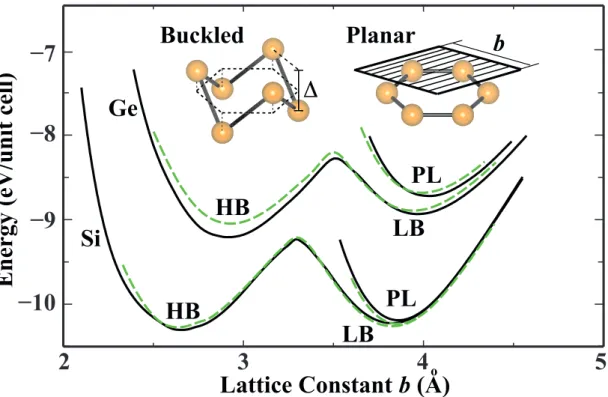
2.3 Energy versus hexagonal lattice constant of 2D Si and Ge are calcu-lated for various honeycomb structures. Black (dark) and dashed green (dashed light) curves of energy are calculated by LDA using PAW potential and ultrasoft pseudopotentials, respectively. Pla-nar and buckled geometries together with buckling distance ∆ and lattice constant of the hexagonal primitive unit cell, b are shown by inset. . . 17

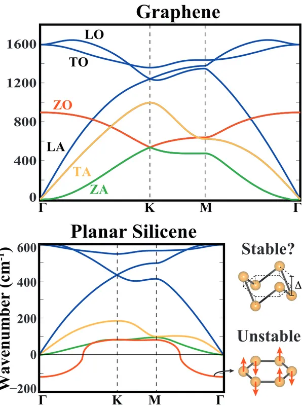
2.4 Phonon dispersion curves of graphene and planar silicene. The lon-gitudinal, transverse and out-of-plane optical and acoustical modes are abbreviated as LO, TO, ZO, LA, TA and ZA, respectively. Eigenvectors corresponding to the out-of-plane optical mode of pla-nar silicene is shown by arrows. . . 19

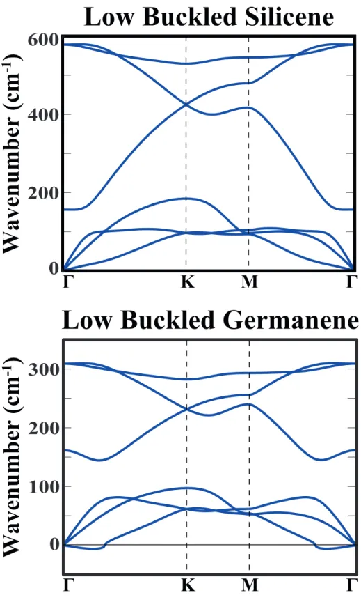
2.5 Phonon dispersion curves for low buckled silicene and germanene structures. . . 21

2.6 Calculated (a) energy gap and (b) effective mass versus ribbon width, n, for hydrogen saturated Si and Ge armchair nanoribbons. Filled circles indicate the ab initio results while empty circles stand for the results of the tight binding fitting. The fitting is performed using only the energy gap data. Parameters found from this fitting was used to generate the tight binding effective mass data. In each panel three branches are observed and named in increasing order of band gaps and effective masses as family I, II, and III. . . 24

2.7 (a) Atomic structure and bond length distribution of hydrogen sat-urated ASiNR-9. (b) Phonon dispersions calculated for hydrogen saturated ASiNR-9. States that appear above 600 cm−1are related to Si-H bonds of hydrogen saturated ASiNR-9 and were not shown. (c) Phonon DOS of the hydrogen saturated ASiNR-9 projected to Si atoms at the center and at the edges and also to H atoms at the edges. DOS of 2D honeycomb structure of Si is also presented for comparison. . . 26

LIST OF FIGURES xii

2.8 Phonon dispersion profiles of cumulene and polyene structures. The number of carbon atoms in the unitcell is given as a subscript. 30

2.9 Forces and difference charge density perturbations formed in finite C100, B50N50 and Al100 atomic chains due to a small longitudinal

displacement, δz, of the 50th atom near the center of the chain. The upper panel is a schematic representation of the geometry of the system. The middle panel presents force distribution for three nearest neighbors (left) and extensions up to 35th neighbor. In the similar manner the bottom panel presents the difference charge density perturbations. Atomic magnetic moments (which are not shown in the figure) also behave similarly, and have long-ranged oscillations in CAC. . . 31

2.10 Energy band structures of AlAl, BB, BN and polyyne chain struc-tures. A closer view of π-bands together with the dispersion pro-file of one-dimensional free electron gas system is presented in the right panel. Zero of energy is set to the minima of π-bands for each structure. For the sake of clarity, the bands of the chain structures beyond the first Brillouin zone in the extended scheme are not shown. 33

3.1 Simple model of electronic friction. (a) Electrons of a metallic block move with velocity v and produce a current density J under the influence of applied electric field E. (b) Atoms are adsorbed on the block and the electrons feel a dissipative force due to interac-tions with adsorbates, as a result electric field has to be increased to produce the same current density J . This can be measured as an increase in the resistivity. (c) In the reference frame of electrons the adsorbates move with velocity v and feel a dissipative force in the opposite direction. . . 39

LIST OF FIGURES xiii

4.1 Simple models of friction. Schematic representation of (a) Prandt-Tomlinson (b) Frenkel-Kontorova and (c) Frenkel-Kontorova-Tomlinson models. (d) Model of two interacting Frenkel-Kontorova chains. The interaction potential is given below the model. . . 43

4.2 Friction force felt by the tip during forward and backward sliding. The model parameters in each case are; (a) ˜γ=4, ˜k=2, ˜v0=0.15

(b) ˜γ=4, ˜k=2, ˜v0=0.05 (c) ˜γ=2, ˜k=2, ˜v0=0.05 (d) ˜γ=0.5, ˜k=0.2,

˜

v0=0.05 (e) ˜γ=0.1, ˜k=0.2, ˜v0=0.05 . . . 45

4.3 Variation of average friction force in (a) Prandtl-Tomlinson and (b) Multichain Frenkel-Kontorova models. . . 47

5.1 Schematic representation of stick-slip regime (left), critical tran-sition (middle) and continuous sliding regime (right) in Prandtl-Tomlinson model. Upper part: the potential energy curves of the surface (green lines) and of the tip(+cantilever) (red lines) ; lower part: force variation of the surface (green lines) and of the tip (red lines). Blue lines represent the potential energy of the tip and sur-face. The magenta dot shows the position of the tip on the surface, while its other end is positioned at the minimum of the parabola shown with red lines in the upper part. The dotted, dashed and solid lines correspond to three different tip positions moving to the right. . . 52

5.2 (a) Ball and stick model showing the honeycomb structure of graphane CH (fluorographene CF) (top) and MoS2 (WO2)

(bot-tom). Calculated values of energy gaps Eg and in-plane stiffness

C are also given in units of eV and J/m2 respectively. (b) Two MoS2 layers sliding over each other have the distance z between

their outermost atomic planes. (c) Each layer is treated as a sepa-rate elastic block. Lateral FL and normal (loading) Fzo forces, the

shear of bottom atomic plane relative to top atomic plane in each layer ∆x(y), and the width of the layer w, are indicated. . . . 53

LIST OF FIGURES xiv

5.3 (a) The contour plot of interaction energy EI of two sliding layers

of MoS2. The zero of energy is set to EI[0, 0, zo(0, 0)]. The energy

profile is periodic and here we present the rectangular unitcell of it. The width of this unitcell in y-direction is equal to the lattice constant a of the hexagonal lattice. Forces in x- (y-) direction is zero along the red (green) dashed lines, respectively. There are several points at which the lateral force ⃗FL, is zero. The arrows

at these critical points indicate the directions where the energy decreases. (b) The energy profiles of EI (blue line) and EIo (red

line) along the horizontal line with Fy = 0 for MoS2. Loading

pressure in all cases is σN=15 GPa. . . 56

5.4 (a) Contour plots of interaction energy EI of two layers of CH, CF,

and WO2 executing sliding motion under constant loading pressure

are presented in their rectangular unit cells. The zero of energy is set to EI[0, 0, zo(0, 0)]. Loading pressure in all cases is σN=15

GPa. (b) Variation of interaction energy E0

I with applied loading

for MoS2 structure along the straight Fy = 0 line passing through

two wells, saddle point and one hill. . . 58

5.5 (a) The force versus shear values along x- and y-directions for each mesh point by red and green dots, respectively. (b) The variation of kc1 and kc2 with loading pressure. (c) The variation of the

frictional figures of merits ks/kc1 and ks/kc2, with loading pressure

calculated for CH, CF, MoS2 and WO2. . . 60

5.6 Calculated lateral force variation of two single layer SiH under two different σN. The top layer is moving to the right or to the left

between two wells. Atomic positions of two SiH layers in stick and slip stages are shown by inset. The movement of SiH layers under loading pressure of σN = 8 GPa is presented as a supplemental

LIST OF FIGURES xv

6.1 (a) Side view of the arrangement of the Ni-ABCBA-Ni structure. The outermost Ni(111) atomic planes are fixed at the separation s. (b) Top view of individual layers constructing the Ni-ABCBA-Ni structure. The primitive unitcell is shown by blue shaded area. Dotted circles represent optimized positions of Ni atoms below the graphene layers in configuration A. . . 66

6.2 Adhesion hysteresis curves for (a) Ni-Ni and (b) Ni-A-Ni structures and its stick-slip behavior shown by inset. (c) Normal force along

z axis as a function of separation s for Ni-graphene-Ni structures

with 2-5 graphene layers. . . 69

6.3 (a) Profiles (contour plots) of potential corrugation for Ni-AA-Ni and AA [without Ni(111) slabs] structures calculated for constant pressure of 7 GPa. The paths along which one slab moves in the course of sliding when pulled along x axis are shown by red dashed lines. The lattice constant of the unit cell is indicated by a. (b) Variation of lateral force Fx along x-axis during sliding of

Ni-AA-Ni structures over the path shown in (a). The sum of areas shaded in green is defined as the corrugation strength WD (see text). (c)

Same as (b) for sliding AA structures without Ni(111) slabs. . . . 71

6.4 (a) Variation of the corrugation strength with number of layers as a function of applied loading pressure for n number of graphene lay-ers (with and without Ni(111) substrates). (b) Perpendicular force

Fz versus the separation distance between outermost graphene

lay-ers for Ni-ABA-Ni and ABA structures (n=3). In the repulsive range, the perpendicular force and hence the potential corrugation is larger in the absence of Ni(111) slabs. . . 73

LIST OF FIGURES xvi

6.5 Isosurfaces and variation of linear density of charge density differ-ence along z-axis. The differdiffer-ence charge density is obtained by sub-tracting the charge densities of Ni slabs and ABA structures from the charge density of Ni-ABA-Ni structure at ∼ 6 GPa. Yellow (blue) isosurface plots correspond to the charge density accumula-tion (depleaccumula-tion). Specific regions of depleaccumula-tion and accumulaaccumula-tion is denoted by numerals on the linear density of charge density differ-ence plot. . . 75

List of Tables

2.1 Binding energy and structural parameters calculated for the bulk and 2D Si and Ge crystals. abulk [in ˚A], Ec,bulk [in eV per atom],

∆HB [in ˚A], ∆LB, bLB, dLB and Ec,LB [in eV per atom],

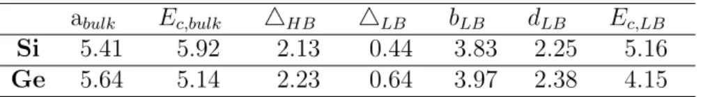
respec-tively, stand for bulk cubic lattice constant, bulk cohesive energy, high-buckling distance, low-buckling distance, hexagonal lattice constant of 2D LB honeycomb structure, corresponding nearest neighbor distance and corresponding cohesive energy. . . 22

Chapter 1

Introduction

This thesis is based on three breakthroughs in physics. The first one is the formulation of the Density Functional Theory (DFT) by pioneering works of Walter Kohn and his collaborators in 1965.[1, 2] This theory provides a rigorous framework for calculation of material properties from first-principles. In this thesis, most of the calculations are performed using DFT.

The second breakthrough is the synthesis of graphene, the first two-dimensional material, by Andre Geim and Konstantin Novoselov in 2004.[3] Be-sides eccentric properties of graphene, like its electrons behaving as massless Dirac Fermions,[4] this was the first realization of a truly two-dimensional mate-rial. This thesis is mainly investigating the frictional and vibrational properties of two-dimensional honeycomb structures like graphene.

The third breakthrough is the invention of the scanning tunnelling microscope by Gerd Binnig and Heinrich Rohrer in 1981,[5] which can be considered as the predecessor of the atomic and friction force microscopes.[6] Having a resolution on the atomic scale, these microscopes boosted the development of the emerging field of nanoscience and nanotechnology. It had impact in most fields of physics including the science of friction and dissipation which is the main topic of this thesis.

CHAPTER 1. INTRODUCTION 2

All these breakthroughs won the Nobel Prize and preserve their importance in the nowadays research. In the forthcoming sections we present a brief information about these breakthroughs and our contributions in the field based on them.

1.1

Density Functional Theory

In 1926, Schr¨odinger published his pioneering paper which included his famous equation marking the beginning of wave mechanics.[7] Shortly after Schr¨odinger‘s equation for electronic wave function, Dirac declared that chemistry had come to an end since all its content was entirely contained in that powerful equation. In principle, all information about the system can be extracted by solving the many-body Schr¨odinger equation;

HΨi(r, R) = EiΨi(r, R) (1.1)

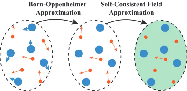
Unfortunately in almost all cases except for the simple systems like He or H, this equation was too complex to allow a solution. The first approximation to this kind of systems is to decouple the motion of electrons and nuclei. This can be done by considering the fact that mass of an ion is at least thousand times higher than mass of an electron while its velocity is thousand times lower. Due to this difference, electrons can arrange themselves according to ionic coordinates before they are changed. In Born-Oppenheimer approximation one can solve the elec-tronic problem by assuming fixed ionic coordinates and then move ions according to the forces due to electronic and ionic distribution, as shown in Fig. 1.1. This leaves us with an electronic problem which is still very hard to solve.

In 1928, first approximation method to solve the electronic problem was pro-posed by Hartree.[8] It postulates that many-electron wave function can be writ-ten as product of one-electron wave functions each of which satisfies one-particle Schr¨odinger equation in an effective potential. In Hartree method, the effective potential itself is determined by one-electron wave functions and one has to per-form iterative calculations until a self-consistent solution minimizing the total energy is reached. This method was then improved to include Pauli exclusion

CHAPTER 1. INTRODUCTION 3

Born-Oppenheimer

Approximation

Self-Consistent Field

Approximation

Figure 1.1: Born-Oppenheimer and Self-Consistent Field Approximations.

principle by writing the total wave function as Slater determinants.[9] The im-proved version is called the Hartree-Fock method and it includes the exchange terms in an exact manner while the many-body correlation terms are completely absent.[10] These kind of methods are in general called self-consistent field approx-imations where an electron is assumed to move under an external interaction field generated by other electrons and ions, as in Fig 1.1. Shortly after Schr¨odinger’s paper, another method was developed by Thomas and Fermi.[11, 12] In Thomas-Fermi approximation the full electron density was taken as the fundamental vari-able of the many-body problem without referring to one-electron orbitals. This approximation did not include exchange-correlation terms and failed to sustain bound states but it set up a basis for Density Functional Theory (DFT).

In 1964, Hohenberg and Kohn introduced the foundation of DFT.[1] In this work they have shown that the full ground state electron density determines all information about the ground state properties of an electronic system. They also state that the total energy of the system can be minimized according to the total electron density instead of electronic wave-functions. This was very impor-tant because it is much simpler to deal with total electron density rather than

CHAPTER 1. INTRODUCTION 4

Initial Guess

Calculate Effective Potential

Solve the Kohn-Sham Equation

Calculate Density

with

Self-Consistent?

YES

NO

Calculate Energy, Forces, Charge Density, etc.

CHAPTER 1. INTRODUCTION 5

full electronic wave-function. In 1965, Kohn and Sham proposed the idea of re-placing the kinetic energy of the interacting electrons with that of an equivalent non-interacting system.[2] This lead to construction of a mathematical object called Kohn-Sham orbitals which minimize the kinetic energy under fixed density constraint. The remaining exchange and correlation terms can be also expressed as a functional of the full electron density, but the exact representation is still not derived. There are two main approximation dealing with these terms. The local density approximation (LDA) and the generalized gradient approximation (GGA). The main idea of LDA is to consider the generally inhomogeneous elec-tronic systems as locally homogeneous and then use the exchange correlation corresponding to the homogeneous electron gas.[13] LDA favors more homoge-neous systems. It over-binds molecules and solids but the chemical trends are usually correct. GGA introduces the inhomogeneties of the density semi-locally, by expanding the exchange-correlation functional as a series in terms of the den-sity and its gradients.[14] GGA improves binding energies, atomic energies, bond lengths and bond angles when compared to the ones obtained by LDA.

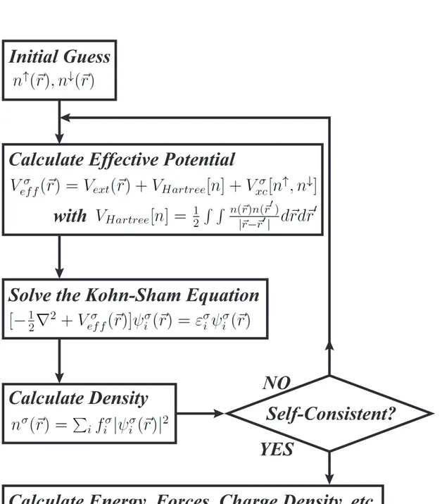
DFT calculations are performed self-consistently as shown in Fig 1.2. For a given configuration of ionic positions one starts with an initial guess of electron density. Then the effective potential corresponding to this density is calculated. The effective potential is then inserted into Kohn-Sham equations to calculate the Kohn-Sham orbitals. Sum of squares of these orbitals multiplied by the oc-cupations gives the new electron density. Obtained new electron density is then compared with the electron density that is used in calculation of effective poten-tial. According to Kohn-Sham ansatz the new and old electron densities should be equal. If their difference is below some acceptable value the self-consistency loop is stopped and one proceeds to the calculation of total energy, forces, charge densities and etc. If the difference is not in the acceptable range the loop is continued until the self-consistency is reached.

The most computationally expensive part of a self-consistent DFT calculation is solution of Kohn-Sham equations. Several numerical approximations are intro-duced here. To deal with the second order derivative in Kohn-Sham equations one can use the reciprocal space discretization.[15] To avoid the rapid oscillations of

CHAPTER 1. INTRODUCTION 6

wavefunction around the ionic singularities one can make use of pseudo-potentials or projector augmentized-wave approximations.[16, 17] Another approximation is expansion of wavefunctions in terms of basis sets which can be plane-waves, gaussians or atomic orbitals. In this thesis, we report DFT results obtained by VASP software which uses plane-waves as a basis set and requires use of periodic boundary condition.[18, 19]

1.2

The Rise of Graphene

Carbon is an element which has a central focus in both life and physical sci-ences. Due to its small core and four valence electrons it can form various types of bondings which result in materials with very different properties. By sp3 hy-bridization C atoms form tetrahedral bonds which build up the diamond struc-ture. In sp2 _{hybridization which is slightly more energetic than sp}3_{, C atoms}

form graphite, fullerene, nanotubes and most of the organic molecules. It can also form sp type hybridization which forms carbon atomic chains. Despite the presence of zero-dimensional (0D) fullerene, one-dimensional (1D) nanotubes and three-dimensional (3D) diamond structures two-dimensional (2D) counterpart of carbon structures were absent until 2004.[3] In fact there was no 2D material synthesized and there were serious doubts about their stability.[36, 37] Synthesis of graphene, the first 2D honeycomb structure of C atoms, revolutionized the physics of 2D materials.

Graphene is the most stiff material due to its strong sp2 _{bonds.[38] However,}

its most exciting properties like planar stability and dashing electronic structure is attained by its pz orbitals. Graphene structure has high carrier concentration

and low impurity scattering which makes it an excellent candidate for ballistic transport devices.[39] Due to the honeycomb symmetry of graphene, its pz

or-bitals have a linear band crossing at the Fermi level which makes electrons act as Massless Dirac Fermions.[4, 40] In the vicinity of the Fermi level carriers obey the relativistic Dirac equation and move with a velocity vF = c/300 ∼ 106 m/s.[41]

CHAPTER 1. INTRODUCTION 7

Paradox and half-integer Quantum Hall Effect.[4, 42, 43]

In our recent work we have shown that Si atoms arranged in a honeycomb lattice cannot remain in planar geometry like graphene but they gain stability via slight puckering.[44] However, this puckering does not break the symmetry re-quired for the linear crossing of π bands and the electronic structure shows similar behavior as that of graphene. The band structure of 2D honeycomb structures of silicon and germanium, now called silicene and germanene, is presented in Chapter 2, where we also discuss the stability of these structures obtained by calculation of their phonon dispersions. Much recently, silicene was synthesized on silver surface and the Fermi velocity of its Dirac electrons was measured.[45]

We have also shown that other Group IV and binary compounds of Group III-V elements can form a stable 2D honeycomb structure.[46] We have found that these structures remain planar as graphene if one of the binary compounds is a member of the first row (i.e. either B, C or N), while the structure attains stability through puckering otherwise, as in case of silicene.

Quasi-1D counterparts of graphene, called graphene nanoribbons, were also synthesized.[47] Their width can reach down to few nanometers. One can build a ballistic transistor using graphene nanoribbons.[48] They have interesting elec-tronic properties attributed to their edge structure. It was shown that graphene nanoribbons having zigzag shaped edges can behave as a half-metal upon applica-tion of an electric field.[49] Graphene nanoribbons having armchair shaped edged have an interesting family behavior in the variation of their band gap versus their width.[50]

We have shown that the family behavior is also present in armchair bons of silicene and germanium.[51] As in the case of armchair graphene nanorib-bons, one can model their band structure in a nearest-neighbor tight-binding scheme of pz orbitals. In Chapter 2, we also discuss the stability of armchair

CHAPTER 1. INTRODUCTION 8

1.3

The Renaissance of Friction

Friction is one of the oldest problems of physics.[20] Early works on the na-ture of frictional forces were done by giants of science widely known for their contributions in other fields like; the painter of Mona Lisa, Leonardo da Vinci; Charles-Augustin de Coulomb of the Coulomb’s law of electrostatics; Leonhard Euler of the Euler’s formula eix _{= cosx + isinx and others.[21, 22] It is no}

sur-prise that friction phenomena attracts so many polymaths from different fields, since here one has to engage complicated microscopic events in an elegant frame-work to account for generally simpler macroscopic behavior. The ultimate theory of friction involves quantum mechanical treatment of events in the atomic scale combined with statistical mechanics to account for the stochastic nature of the problem.

In early experimental works, the friction force was found to be nearly inde-pendent of the apparent area of contacts and sliding velocity. It was also found that, the friction force has a linear dependence on the applied loading force. Even though deviations from these results are rarely observed in everyday life the underlying physics is not at all obvious. In fact, there was no rigorous un-derstanding of them until 1940s. Friction force was also found to depend on the time the surfaces remained in stationary contact (history of sliding) and ambient conditions like temperature, humidity, etc. A detailed historical review of early works on friction can be found elsewhere.[23] Here we would like to point out some important aspects of these works.

Until the work by Prandtl (1928) and Tomlinson (1929) it was not clear why in certain cases friction force had weak dependence on sliding velocity.[24, 25] In the case of a rigid object moving in a viscous fluid, Stokes’ law dating back to 1851 established a drag force which was proportional to the velocity of the particle. Prandtl-Tomlinson model showed that when the sliding surfaces have high corrugation or low stiffness the relative motion enters in a stick-slip regime. Here the surfaces first cling to each other and when they reach some critical strain the stored elastic energy is released as rapid atomic movements. Their model shows that for a reasonable range of sliding velocities, friction force undergoes a

CHAPTER 1. INTRODUCTION 9

Sliding Velocity

S

ti

ffn

es

s/

C

or

ru

gati

on

Stick-Slip Regime

Superkinetic Regime

Drag Regime

Steady or Continuous

Sliding Regimes

Figure 1.3: General dependence of friction regimes on sliding velocity and ratio of stiffness to the corrugation potential. In the drag regime, friction force is pro-portional to velocity while in the superkinetic regime it is inversely propro-portional. In the stick-slip regime friction force has weak dependence on sliding velocity. For each regime, a sketch of surface asperities is presented.

minor change. The details of this model is discussed in Chapter 4.

Another issue was to resolve why the friction force had minor dependence on surface area and why it was proportional to applied loading. In 1940, Bowden and Tabor resolved these issues by introducing the concepts of apparent and real area of contact.[26] They have shown that the microscopic asperities of the surface that were actually in a contact made up much smaller area, called real area of contact, compared to the are that was measured macroscopically or apparent area. They have also shown that the real area of contact was proportional to applied loading force and the friction force was proportional with real are of contact. Here the effect of increasing the loading force was not to increase the area of already present junction (which would lead to a nonlinear dependence of real area on loading force) but to increase the number of junctions.[27] This explained why the friction force was independent of apparent area and why it

CHAPTER 1. INTRODUCTION 10

was proportional to applied loading force.

In his book,[20] Persson ironically points out an infertile period in friction science from 1960 to 1987 in which surface scientists were attracted by simpler phenomena like adsorption of atoms and molecules on single crystal surfaces. However, one of such debates was resolved with a tool that would revolutionize many fields including the friction science. This debate was the reconstruction nature of Si(111) surface. Experiments were pointing on a (7x7) reconstruction which was very hard to analyse in detail by experimental and computational tools of that time. In 1983, Binnig et al. resolved this issue using the scanning tunneling microscope introduced by themselves.[5, 28] In 1986, Binnig et al. in-troduced atomic force microscope which was used in a first atomic scale friction experiment.[6]

The renaissance of friction and emergence of nanotribology was kindled in 1987, by the first experiment on the atomic scale friction.[29] In their seminal paper, Mate et al. used an atomic force microscope with a tungsten tip which was slid over a graphite surface.[30] They have shown that the friction force detected by the microscope had atomic-scale features like stick-slip with a periodicity of graphite lattice. They also were able to detect double-slips occurred during sliding of the tip. Results of this experimental work was then investigated in the context of Prandtl-Tomlinson model.[31] These works were followed by vast amount of experimental and theoretical papers on atomic scale friction but here we would like to mention only some of them.

Transition from stick-slip to continuous sliding in atomic scale friction was investigated by Socoliuc et al., using friction force microscope.[32] They have shown that when the loading force is decreased below some critical value the stick-slip regime ends and the system enters in the ultralow friction regime. They give explanation to this transition using the Prandtl-Tomlinson model. Here the corrugation potential is proportional to applied loading and when the curvature of the corrugation potential falls below the stiffness of the tip, it starts to move without making any sudden jumps. Further details of this transition is presented in Chapter 4.

CHAPTER 1. INTRODUCTION 11

In our study, presented in Chapter 5, we have developed a method for calcu-lation of intrinsic stiffness and corrugation potential between layered structures under constant loading pressure. We have combined the stiffness and the criti-cal curvature derived from the corrugation potential in a single quantity criti-called frictional figure of merit.[33] Analysing this quantity, which is a material prop-erty under certain loading pressure, we have shown that the oxidation resistant tungsten oxide structure can be better lubricant than the well established molyb-denum disulfide structure.

Transition from stick-slip to steady sliding regime is also observed when sliding velocities exceed certain critical values. In this case the system enters in the super-kinetic regime where the friction force generally decreases when the sliding velocity is increased.[34] This kind of behavior is also observed in our simple model described in Chapter 4. Both of the mentioned transitions can be analysed by plotting a dynamical phase space of the system, as shown in Fig 1.3.[35] The nature of these transitions, like if they are continuous or discontinuous, is one of the fundamental problems of nowadays friction science.

1.4

Organization of the Thesis

This thesis is composed of two main parts. In the first part, stability and vibra-tional properties of various materials like 2D silicene, quasi-1D silicene nanorib-bons and carbon atomic chains are discussed. This part is presented in Chap-ter 2. In the second part, frictional properties of layered lubricants are presented. Chapters 3 and 4 summarize crucial aspects of friction science like phononic and electronic dissipation, adiabatic and sudden processes, Prandtl-Tomlinson model, and etc. Discussions provided in these chapters are critical for understanding of Chapter 5 which contains our main contribution in the field. In Chapter 5, we introduce the concept of frictional figure of merit and predict the performance potential of new lubricant materials. In Chapter 6, we discuss potential corruga-tion of multilayer graphene structures. The concluding remarks are presented as an outlook in Chapter 7.

Chapter 2

Phonons and Stability

In this chapter, the basic concept of phonons and the methods for calculation of phonon dispersions is introduced. We also present our recent works, in which we use phonon spectra as stringent test of stability and predict the possibility of materials having interesting electronic properties. Phonon calculation presented here also reveal some interesting physics like fourth acoustical mode in quasi-1D nanoribbons and Friedel oscillations which give rise to long-ranged interactions in 1D atomic chains.

2.1

Introduction

Matter is composed of atoms vibrating around a certain equilibrium position determined by positions of neighboring atoms. This vibrations are resulted by restoring forces that atoms feel when they are displaced from their equilibrium position. This collective motion of atoms can be quantized into an entity which behaves as a particle called phonon. Phonons possess energy and momentum which can be measured, for example, by neutron scattering. Phonons behave as bosonic particles which obey the Bose-Einstein statistics. Observation of a single phonon is very challenging and was achieved only very recently.[52]

CHAPTER 2. PHONONS AND STABILITY 13

m

m

m

m

m

m

u

u

u

u

u

u

C

a

Figure 2.1: Diatom chain with harmonic interactions.

To determine phonon dispersion and phonon-phonon interaction cross-sections one has to know the variation of restoring force with displacement of each atom in a unitcell of a crystal.[53] In the following section we present a formalism for calculation of phonon dispersion in harmonic approximation where the magni-tude of the restoring force is assumed to be proportional to the magnimagni-tude of displacement.

2.2

Dynamical Matrix Formulation

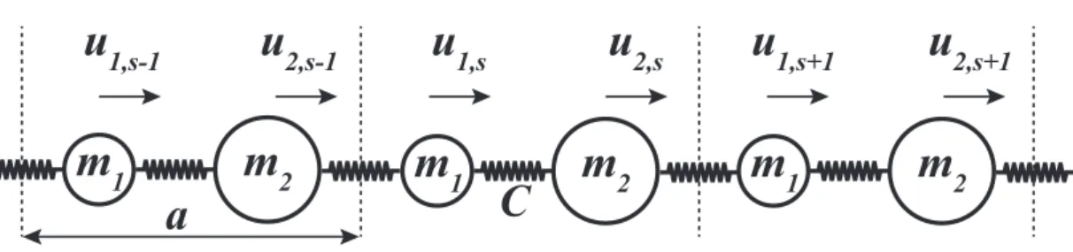
We start by a simple example of one-dimensional diatomic crystal with harmonic nearest neighbor interactions, as shown in Fig. 2.1.[54] Equations of motion for this system can be written as;

m1u¨1,s= C(u2,s−1− u1,s) + C(u2,s− u1,s) m2u¨2,s= C(u1,s+1− u2,s) + C(u1,s− u2,s)

(2.1)

these coupled differential equations have solutions of the form;

ui,s = vi eiωt+iska with i ={1, 2} (2.2)

where vi is the amplitude of vibration of ith atom and k is the wave-vector.

Inserting (2.2) into (2.1) leads to a matrix eigenvalue problem;   2C/m1 C(1 + e−ika)/m1 C(1 + eika)/m2 2C/m2     v1 v2  _{= ω}2   v1 v2   _(2.3)

CHAPTER 2. PHONONS AND STABILITY 14

which can be rewritten in a more symmetric way as;   2C/ √ m1m1 C(1 + e−ika)/√m1m2 C(1 + eika_)/√_m 2m1 2C/√m2m2     √ m1v1 √ m2v2  = ω2   √ m1v1 √ m2v2  . (2.4) Here the two by two matrix in the left hand side is called the Dynamical Matrix. Eigenvalues of Dynamical Matrix give dispersions of phonon branches in terms of ω(k)2_{. The number of phonon branches is equal to the degrees of freedom}

which is also the size of the Dynamical Matrix. In this simple case there are two phonon branches. One of these branches is acoustical and one is optical. In general, the number of acoustical branches equals to the number of possible invariant transformation. In the case of diatomic chain the system can be shifted along the axis and stay invariant. Frequencies of acoustical modes are zero at the center of the Brillouin zone, since there is no restoring force acting against an invariant transformation. In the light of equation (2.4), one can generalize the Dynamical Matrix to a 3D crystal with interaction which are not necessarily confined to nearest neighbors, as following;

Dsα,tβ = 1 √ msmt ∑ n,l Φnsα,ltβ ei⃗k·( ⃗Rltβ− ⃗Rnsα) (2.5)

where Dsα,tβ is dynamical matrix element due to the force in cartesian coordinate

α felt by sth atoms in the unitcells resulting from the movement of tth atoms in the unitcells in cartesian coordinate β. In similar fashion, Φnsα,ltβ is the force

constant which corresponds to the ratio of the felt force to the magnitude of the displacement, where indices n and l denote the unitcells. ⃗Rnsα and ⃗Rltβ are

position vectors while ⃗k is the wave-vector. The summation should be performed over all unitcells which possess finite interaction. Derivation of (2.4) from (2.5), which is left to the reader, can be very usefull for understanding the Dynamical Matrix formalism.

2.3

Small Displacement Method

In the following sections we present a recipe for performing phonon dispersion calculation using DFT combined with Dynamical Matrix formalism introduced

CHAPTER 2. PHONONS AND STABILITY 15

in the previous section. The idea is to derive the force constant matrix by dis-placing atoms in sufficiently large unitcells which include all interacting neighbors and calculate the resulting Hellmann-Feynman forces due to these displacements. Using the symmetry of the system one can reduce the number of displacements needed for this derivation. Throughout the work presented in this thesis we have used the freely available PHON program[55] for calculation of phononic properties from forces calculated by the widely used DFT software VASP.[56]

To obtain a reliable phonon spectra one needs to tune the calculation pa-rameters accordingly. In this respect, we present phonon calculations of several important materials. Besides their interesting electronic properties, phonon anal-ysis of these materials helps to explore interesting phenomena like stability of 2D silicene through puckering, forth acoustical mode in quasi-1D nanoribbons and long-ranged interaction in 1D carbon atomic chains.

2.4

Stability of Silicene

The unusual electronic properties of graphene, which is derived from its pla-nar honeycomb structure leads to charge carriers resembling massless Dirac fermions.[4, 40] Recent synthesis of graphene has demonstrated that this truly two dimensional (2D) structure is stable and has introduced novel concepts.[3, 43, 57, 58, 59] Not only the fundamental properties of 2D graphene, but also interesting size and geometry dependent electronic and magnetic properties of their quasi 1D nanoribbons have been revealed.[47, 48, 49, 50] While the research interest on graphene and its ribbons is growing rapidly, one has started to ques-tion whether the other Group IV elements in Periodic Table, such as Si and Ge, have stable honeycomb structure. Even before the synthesis of isolated graphene, ab-initio studies based on the minimization of the total energy has revealed that a buckled honeycomb structure of Si can exists.[60, 61, 62]

In this section, based on the atomic structure optimization and phonon dis-persion calculations we show that the low-buckled honeycomb structures of Si and

CHAPTER 2. PHONONS AND STABILITY 16

6

3

-6

-3

0

6

3

-6

-3

0

M K

Γ

En

e

r

gy (e

V

)

DOS

Si-LB

Ge-LB

0.4

0.0

-0.4

0.4

0.0

-0.4

p

_x

K

"

Γ

"

*

"

"

*

"

*

"

"

*

"

p

_y

s

p

_x

p

_y

s

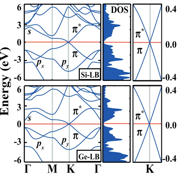
Figure 2.2: Energy band and density of states (DOS) diagrams of low-buckled (LB) 2D honeycomb structures Si and Ge. The crossing of the π and π∗ bands at

K- and K′-points of BZ is amplified to show that they are linear near the cross section point. Zero of energy is set at the Fermi level, EF. Orbital character of

CHAPTER 2. PHONONS AND STABILITY 17

2

3

4

5

−10

−9

−8

−7

Lattice Constant b (A)

En

er

gy (e

V

/u

n

it c

el

l)

Si

Ge

HB

LB

PL

HB

PL

LB

Buckled

Planar

_b

Δ

Figure 2.3: Energy versus hexagonal lattice constant of 2D Si and Ge are calcu-lated for various honeycomb structures. Black (dark) and dashed green (dashed light) curves of energy are calculated by LDA using PAW potential and ultra-soft pseudopotentials, respectively. Planar and buckled geometries together with buckling distance ∆ and lattice constant of the hexagonal primitive unit cell, b are shown by inset.

Ge are stable. Similar to graphene, their π- and π∗- bands cross linearly at the Fermi level at the K- and K′-(Dirac) points of the hexagonal Brillouin zone (BZ), as seen in Fig.2.2. The bands display an ambipolar character and the charge carriers behave like massless Dirac fermions in a small energy range around the Fermi level, EF.

Here we have performed first-principles plane wave calculations within Local Density Approximation (LDA)[66] using PAW potentials[67] as well as ultrasoft pseudopotentials.[16] All structures have been treated within supercell geometry using the periodic boundary conditions. A plane-wave basis set with kinetic energy cutoff of 500 eV is used. In the self-consistent potential and total energy calculations the Brillouin zone (BZ) is sampled by (25×25×1) special k-points.[15]

CHAPTER 2. PHONONS AND STABILITY 18

This sampling is scaled according to the size of supercells. All atomic positions and lattice constants are optimized by using the conjugate gradient method where total energy and atomic forces are minimized. The convergence for energy is chosen as 10−5 eV between two steps, and the maximum force allowed on each atom is less than 10−4 eV/˚A. Phonon dispersion curves obtained using Small Displacement Method with forces calculated by VASP.[18, 19, 55, 56]

Calculated variation of the binding energy of the relaxed honeycomb structure of Si and Ge as a function of the lattice constant is presented in Fig.2.3. Here planar (PL), low-buckled (LB) and high buckled (HB) honeycomb structures correspond to distinct minima. The PL honeycomb structure is the least energetic configuration. The important question to be addressed is whether these PL, LB and HB geometries correspond to real local minima in the Born-Oppenheimer surface and hence are stable.

We start by calculation of phonon dispersions of planar silicene and germanene structures. Phonon dispersions corresponding to graphene and planar silicene structures are presented in Fig.2.4. Here one can see that the main difference between these two profiles are in their out-of-plane optical modes. As seen in, Fig.2.4 the eigenvector corresponding to this mode is composed of opposite out-of-plane motion of atoms in each sublattice. In graphene structure there is a strong restoring force against this movement which results in oscillation with wavenumber around 900 cm−1 at Γ-point. In the case of planar silicene there is no restoring force against such movement and this results in imaginary frequencies with amplitudes more than 100 cm−1 at Γ-point. This instability can be cured by letting the silicon atoms move towards directions in which they do not feel a restoring force, i.e., by letting the silicene structure buckle.

The phonon dispersion curves in Fig.2.5 indicate that 2D periodic LB hon-eycomb structure of Si is stable since imaginary frequencies are absent. With an equilibrium buckling ∆LB=0.44 ˚A, its optical and acoustical branches are well

CHAPTER 2. PHONONS AND STABILITY 19

K

M

Wave

n

u

mb

er

(c

m

-1

)

Г

Г

0

400

800

1200

1600

Graphene

LA

TA

ZA

ZO

LO

TO

−200

0

200

400

600

K

M

Δ

Г

Г

Planar Silicene

Unstable

Stable?

Figure 2.4: Phonon dispersion curves of graphene and planar silicene. The longi-tudinal, transverse and out-of-plane optical and acoustical modes are abbreviated as LO, TO, ZO, LA, TA and ZA, respectively. Eigenvectors corresponding to the out-of-plane optical mode of planar silicene is shown by arrows.

CHAPTER 2. PHONONS AND STABILITY 20

branch displays a quadratic dispersion near Γ-point, since the force constants re-lated with the out-of-plane motion of atoms decays rapidly.[56] The phonon dis-persion curves of 2D periodic LB structure of Ge having a buckling of ∆LB=0.64

˚

A are similar to those of Si, except the frequencies of Ge are almost halved due to relatively smaller force constants. The out-of-plane acoustical phonon branch has imaginary frequencies near Γ-point. We have shown that these frequencies become positive when the grid size of the real space mesh is reduced. This way the forces are calculated more precisely.

The stability of LB structure of Si and Ge is further tested by extensive ab-initio finite temperature molecular dynamics calculations using time steps of

δt = 2×10−15seconds. In these calculations the (4×4) supercell is used to lift the constraint of (1×1) cell. Periodic 2D LB structure of Si (Ge) is not destroyed by raising the temperature from T = 0 to 1000 K (800 K) in 100 steps, and holding it at T = 1000 K (800 K) for 10 picoseconds (ps). A finite size, large hexagonal LB flake of Si (Ge) with hydrogen passivated edge atoms is not destroyed upon raising its temperature from 0 to 1000 K (800 K) in 100 steps and holding it for more than 3 ps.

As in the PL case, HB honeycomb structures of Si and Ge, with a buckling of ∆HB ≈ 2 ˚A, also have imaginary phonon frequencies for a large portion of BZ.

Moreover, structure optimization of HB structure on the (2×2) supercell results in an instability with a tendency towards clustering. Clearly, the unstable HB structure does not correspond to a real local minimum; it can occur only under the constraint of the (1×1) hexagonal lattice.

We believe that the present analysis provides stringent and comprehensive test for the stability of LB honeycomb structure of both Si and Ge. In this respect, LB structures of Si and Ge appear to be a contrast to 2D C and BN forming only stable planar honeycomb structure.[46] The situation with three different minima corresponding to PL, LB and HB geometries of 2D Si and Ge in Fig.2.3 is reminiscent of those of 1D atomic chains. Earlier, it has been shown that while several elements and III-V compounds form linear, wide-angle (i.e. LB) and low-angle (i.e. HB) atomic chains, only C and BN form stable linear

CHAPTER 2. PHONONS AND STABILITY 21

0

200

400

600

0

100

200

300

Wave

n

u

mb

e

r

(c

m

-1

)

Low Buckled Silicene

K

M

Г

Г

Low Buckled Germanene

K

M

Г

Г

Wave

n

u

mb

e

r

(c

m

-1

)

Figure 2.5: Phonon dispersion curves for low buckled silicene and germanene structures.

CHAPTER 2. PHONONS AND STABILITY 22

Table 2.1: Binding energy and structural parameters calculated for the bulk and 2D Si and Ge crystals. abulk [in ˚A], Ec,bulk [in eV per atom], ∆HB [in ˚A], ∆LB,

bLB, dLB and Ec,LB [in eV per atom], respectively, stand for bulk cubic lattice

constant, bulk cohesive energy, high-buckling distance, low-buckling distance, hexagonal lattice constant of 2D LB honeycomb structure, corresponding nearest neighbor distance and corresponding cohesive energy.

abulk Ec,bulk △HB △LB bLB dLB Ec,LB

Si 5.41 5.92 2.13 0.44 3.83 2.25 5.16

Ge 5.64 5.14 2.23 0.64 3.97 2.38 4.15

atomic chains.[63, 64, 65] That only C and BN form linear 1D atomic chains and 2D planar honeycomb structures arises from the limited size of their 2s and 2p valance orbitals. Whereas elements from the second and third row of the Periodic Table have 2s and 2p orbitals as core states and the range of their valance orbitals is large enough to yield significant second nearest neighbor coupling. Relevant lattice parameters and cohesive energies of LB Si and Ge honeycomb structures are given in Table 2.1. Different potentials (PAW or ultrasoft pseudopotential) yielded values which differ only 1%. We note that the cohesive energies of LB structures are smaller than those for the bulk crystal of Si and Ge.

The calculated electronic band structures and corresponding density of states (DOS) of LB Si and Ge are presented in Fig.2.2. The bands of PL and LB structures are similar except that specific degeneracies split due to lowering of point group rotation symmetry from C6 in PL geometry to C3 in LB geometry.

Similar to graphene, π- and π∗-bands of LB Si and Ge crossing at K- and K′ -points at EF are semimetallic. Around the crossing point, these bands are linear.

This behavior of bands, in turn, attributes a massless Dirac fermion character to the charge carriers. Interestingly, by neglecting the second and higher order terms with respect to q2, the Fermi velocity is estimated to be vF ∼ 106 m/s for

both Si and Ge. We note that vF calculated for LB honeycomb structures of Si

and Ge are rather high and close to that of graphene. In addition, because of the electron-hole symmetry at K- and K′-points of BZ, LB Si and Ge are ambipolar for E(q)= EF ± ϵ, ϵ being small.

CHAPTER 2. PHONONS AND STABILITY 23

Much recently, a compelling experimental evidence for the synthesis of epitax-ial silicene on a silver (111) substrate was provided.[45] Using scanning tunnelling microscopy and angular-resolved photoemission spectroscopy the authors have re-vealed the structural and electronic properties of silicene, which are in a very good agreement with our predictions.

2.5

Fourth Acoustic Mode in Nanoribbons

Freestanding graphene sheets and nanoribbons can be produced spontaneously, but it is not the case for silicene and germanene. However, there are plenty exper-imental work on growth of Si nanoribbons especially on Ag surface.[68, 69, 70, 71, 72, 73, 74] These highly metallic nanoribbons are formed by self-organization and have straight, atomically perfect and massively parallel structures. The electronic structure of Si nanoribbons on Ag surface was also investigated theoretically.[75] As mentioned in Chapter 1, similar to armchair graphene nanoribbons, armchair silicene nanoribbons (ASiNR) also possess family behavior (see Fig 2.6) in the variation of their band gap with their width.[50] We have shown that this property of ASiNR can be used to build multiple quantum well structures by periodically modifying their width.[51]

One can model the band structure of armchair silicene nanoribbons in a nearest-neighbor tight-binding scheme of pz orbitals. Here the hopping

param-eters, t, is taken to be the same between all nearest-neighbor atoms except the edge atoms in which it should be modified as t(1 + δ). The results of ab initio calculations and parametrized tight-binding calculations are presented in Fig 2.6. It is worth to note here that, the value of δ for silicene nanoribbons was found to be 0.12 which is the same as the value reported for the graphene nanoribbons.[50]

In this section we present stability analysis of ASiNR, based on the calculation of the phonon dispersions. We have performed first-principles plane wave calcu-lations within Local Density Approximation (LDA) using projector augmented

CHAPTER 2. PHONONS AND STABILITY 24 1.0 0.0 0.2 0.4 0.6 0.8 tight-binding ab initio

En

er

gy G

ap

(e

V

)

Ribbon Width “n”

H passivated ASiNR

H passivated AGeNR

tight-binding ab initio 0.0 1.0 2.0 3.0

Effe

cti

ve

M

as

s (m )

(a)

(b)

I

II

III

I

II

III

I

II

III

I

II

III

Figure 2.6: Calculated (a) energy gap and (b) effective mass versus ribbon width,

n, for hydrogen saturated Si and Ge armchair nanoribbons. Filled circles indicate

the ab initio results while empty circles stand for the results of the tight binding fitting. The fitting is performed using only the energy gap data. Parameters found from this fitting was used to generate the tight binding effective mass data. In each panel three branches are observed and named in increasing order of band gaps and effective masses as family I, II, and III.

CHAPTER 2. PHONONS AND STABILITY 25

wave (PAW) potentials.[66, 67] All structures are treated within supercell geom-etry using the periodic boundary conditions. A plane-wave basis set with kinetic energy cutoff of 300 eV is used. In the self-consistent potential and total energy calculations, the Brillouin zone (BZ) is sampled by (15× 1 × 1) special k-points. All atomic positions and lattice constants are optimized by minimization of the total energy and atomic forces. The vacuum separation between the nanoribbons in the adjacent unit cells is taken to be at least 10 ˚A. The convergence for energy is chosen as 10−5 eV between two steps, and the maximum Hellmann-Feynman forces acting on each atom is less than 0.02 eV/˚A upon ionic relaxation. Numeri-cal plane wave Numeri-calculations have been performed by using VASP package.[18, 19] Phonon dispersions were obtained using the small displacement method with forces calculated in a (5× 1 × 1) supercell.[55, 76]

Figure 2.7(a) presents the atomic structure and bond length distribution of a sample hydrogen saturated armchair silicon nanoribbons. In contrast to bare nanoribbons, saturation by hydrogen lifts the (2×1) reconstruction at the edges.[44] In Fig. 2.7(a) there are n = 9 Si atoms forming zigzag chain perpen-dicular to the nanoribbon axis and hence this armchair nanoribbon is classified as ASiNR-9. Accordingly the number of Si (or Ge) atoms in the primitive unit cell is 2n. Note that the bond length distribution is nearly uniform except a sud-den decrease at the edges. This pattern was also observed in armchair graphene nanoribbons.[50]

Figure 2.7(b) presents the phonon dispersion profile for hydrogen saturated ASiNR-9. In the phonon dispersion profile of hydrogen saturated ASiNR-9 all modes are real. Thus, the structure is predicted to be stable. Computational cost of this calculation is very high, so we were not able to calculate the phonon dispersions for other ribbons. Nevertheless, all ASiNRs have very similar atomic configuration, and thus they are also expected to be stable. As seen in Fig 2.5 the phonon dispersion profile of 2D Ge is similar to that of Si. But in Ge structure the acoustic and optic modes are well separated. Also due to softer bonds the wavenumbers of Ge structure is halved compared to Si. Thus AGeNRs are also expected to be stable, whilst exhibiting the mentioned differences.

CHAPTER 2. PHONONS AND STABILITY 26

(b)

W

av

en

u

mb

er

(c

m

)

0

200

400

600

ASiNR-9

Γ

X

0

100

200

300

400

500

600

700

Wavenumber (cm

₎

Two dimensional Si

ASiNR-9 Si atoms at the center

ASiNR-9 Si atoms at the edges

ASiNR-9 H atoms at the egdes

P

h

on

on

D

O

S

(

ar

b

. u

n

its

)

(c)

(a)

H passivated Bond Length (Å)

2.2

2.3

2.4

Si

Ge

n

=9

Figure 2.7: (a) Atomic structure and bond length distribution of hydrogen saturated ASiNR-9. (b) Phonon dispersions calculated for hydrogen saturated ASiNR-9. States that appear above 600 cm−1 are related to Si-H bonds of hydro-gen saturated ASiNR-9 and were not shown. (c) Phonon DOS of the hydrohydro-gen saturated ASiNR-9 projected to Si atoms at the center and at the edges and also to H atoms at the edges. DOS of 2D honeycomb structure of Si is also presented for comparison.

CHAPTER 2. PHONONS AND STABILITY 27

Interestingly, in quasi-1D structures like ASiNR there are four acoustical modes, which is in contrast to 2D and 3D structures which possess three acous-tical modes. As mentioned before, the number of acousacous-tical modes is equal to the number of invariant transformations. In the case of quasi-1D nanostructures the fourth acoustical mode is originating from the rotational invariance that these materials have. In this respect, four phonon modes of ASiNR have zero frequency as they approach the Γ-point. The acoustic mode corresponding to the rotational invariance is usually called the twisting mode (TW).[77, 78]

Usually, acoustical modes does not converge to exactly zero due to finite numerical precision. In this case one can apply the following recursive procedure to impose the invariant symmetries to dynamical matrix;

Dnew = D_old− (D_oldvvT + vvTD_old)/2 (2.6)

where, D_old and D_new are old and new value of the dynamical matrix in each iteration and v is the eigenvector corresponding to invariant transformation.[78] In the case of quasi-1D structures there are three such eigenvectors corresponding to translation in Cartesian coordinates and one corresponding to rotation around the axis in which the structure is periodic. Generally sufficient precision is reached by using the recursion formula (2.6) in less than 20 iterations.[55]

Phonon densities of states (DOS) of hydrogen saturated ASiNR-9 projected to atoms at different locations in the nanoribbon are presented in Fig. 2.7(c). DOS of the 2D Si honeycomb structure is also presented for comparison. DOS projected on Si atoms at the center of the nanoribbon is very similar to that of the 2D Si. As the width of the nanoribbon increases, this similarity is expected to be enhanced. However, DOS projected on Si atoms at the edges deviate from that corresponding to 2D Si. Especially, four optical peaks above 600 cm−1 are clearly originating from Si-H bonds at the edges. Also modes originating from short Si-Si bonds at the edges cause changes in DOS below 600 cm−1.