On the structure and implementation of the optimal Q-Parameter in the one-block H-infinity control problem

ON THE STRUCTURE AND

IMPLEMENTATION OF THE OPTIMAL

Q-PARAMETER IN THE ONE-BLOCK

H-INFINITY CONTROL PROBLEM

A THE SIS SUBM IT TE D TO

THE GRADUATE S CHO O L O F E NGINE E RING AND SC IE N CE O F BIL K E NT UNIV E RSITY

IN P ARTIAL FUL FI L L ME NT O F THE RE Q UIRE ME NTS FO R THE DE GRE E O F

MASTE R O F SC IE N CE IN

E L E CTRICAL AND E L E CTRO NICS E N GINE E RING

By

Çetin Taştekin

November 2020

ii

On the Structure and Implementation of the Optimal Q-Parameter in the One-Block H-Infinity Control Problem

By Çetin Taştekin November 2020

We certify that we have read this thesis and that in our opinion it is fully adequate, in scope and in quality, as a thesis for the degree of Master of Science.

Hitay Özbay (Advisor)

Ömer Morgül

Mehmet Önder Efe

Approved for the Graduate School of Engineering and Science:

Ezhan Karaşan

iii

ABSTRACT

ON THE STRUCTURE AND

IMPLEMENTATION OF THE OPTIMAL

Q-PARAMETER IN THE ONE-BLOCK

H-INFINITY CONTROL PROBLEM

Çetin Taştekin

M.S. in Electrical and Electronics Engineering Advisor: Hitay Özbay

November 2020

In the robust control theory, 𝐻_∞ methods are carried out to procure so-lutions to sensitivity minimization (nominal performance) and robust stabil-ity problems in general. These one – block control problems can be analyzed separately or in a combined fashion. In the general sense, the design of the robust controller is made to achieve stability and performance objectives for a plant, whose nominal model and uncertainty bounds can be determined from the experimental data.

This study aims to present a solution to infinite dimensional one – block 𝐻∞ control problem and provide a general structural result for Q – Param-eter. The methods like Nevanlinna – Pick interpolation will not work for infinite dimensional control problems whereas Sarason’s Theorem provides solution to infinite dimensional control problems. In this thesis, Sarason’s Theorem is analyzed and examined extensively and applied on infinite di-mensional one – block 𝐻_∞ control problem.

The detailed structural analysis of the resulting Q – Parameter is made as the main contribution of the thesis. Various examples are given to illus-trate the computational issues. In this analysis, stability status of Q – Pa-rameter is demonstrated by examining stable terms and FIR part of its sub – blocks.

iv

Keywords: Robust control, one - block 𝐻_∞ control problem, 𝐻_∞controller, infinite dimensional systems, Sarason’s Theorem, Q - Parameter.

v

ÖZET

TEK-BLOK H-SONSUZ

KONTROL PROBLEMİNDE

OPTİMAL Q-PAREMETRESİNİN

YAPISI VE UYGULAMASI

Elektrik ve Elektronik Mühendisliği, Yüksek Lisans Tez Danışmanı: Hitay Özbay

Kasım 2020

Gürbüz kontrol teorisinde, 𝐻_∞ yöntemleri, genel olarak hassaslık mini-mizasyonu (nominal performans) ve gürbüz kararlılık problemleri için çözümler sağlamak amacıyla uygulanır. Bu tek bloklu kontrol problemleri, ayrı ayrı analiz edilebilir veya birlikte incelenebilir. Genel anlamda, deneysel verilerden belirlenebilen nominal bir sistem ve belirsizlik altında kararlılık ve performans hedeflerine ulaşmak için gürbüz kontrolcü tasarımı yapılır.

Bu çalışma, sonsuz boyutlu tek bloklu 𝐻_∞ kontrol problemine bir çözüm ortaya koymayı ve Q – Parametresi için genel bir yapısal sonuç sunmayı amaçlamaktadır. Nevanlinna - Pick interpolasyonu gibi yöntemler sonsuz boyutlu kontrol problemlerinde çalışmazken, Sarason Teoremi sonsuz boyutlu kontrol problemlerine çözüm sağlar. Bu bağlamda, Sarason Teoremi kapsamlı bir şekilde analiz edilip incelenerek, sonsuz boyutlu tek bloklu 𝐻_∞ kontrol problemine uygulanmıştır.

Tezin ana katkısı, elde edilen Q - Parametresi’nin detaylı yapısal anali-zidir. Hesaplama meselelerinin canlandırması için çeşitli örnekler verilmiştir. Bu analizde, Q - Parametresinin kararlılık durumu, yapısının kararlı terim-leri ve FIR kısmı incelenerek gösterilmiştir.

Anahtar sözcükler: Gürbüz kontrol, tek - blok 𝐻_∞ kontrol problemi, 𝐻_∞ kontrolcüsü, sonsuz boyutlu sistemler, Sarason Teoremi, Q - Parametresi.

vi

Acknowledgement

First of all, I would like to express my endless gratitude to my advisor Professor Hitay Özbay. In the most hopeless period of my graduate educa-tion, he accepted to be my advisor. He just believed in me and helped me, just like a father. There are no simple words to tell how I respect him. He will always remain as a father and the greatest role model for me in my whole life. His understanding, patience, absolute knowledge and immense support are priceless and most precious for me and my graduate education. Today, if this work exists, it is because of him. It was an honor to be his M.Sc student and have a chance to work with him. I will be always appre-ciated.

I would like to thank Professor Mehmet Önder Efe and Professor Ömer Morgül for reading my thesis and guiding me in the thesis committee.

I also want to thank Professor Süleyman Serdar Kozat for supervising me at the beginning process of my graduate education. As my undergraduate advisor and respected instructor, his assistance was invaluable to shape my graduate study. Special thanks to Professor Arif Bülent Özgüler for accept-ing me as M.Sc student in the first place and constant support duraccept-ing my studies.

I would like to state my sincerest thanks and gratefulness to my parents, Gülen and İsmet Kemal Taştekin, and also my brother Osman Taştekin. Besides, I am grateful and beholden to my precious grandmother, Kadriye Soysal. With their endless support, I become who I am right now. I also want to express my special thanks and appreciation to my mother and father in law, Ferhan and Sadık Sezai Karaköse. They always backed me up and encourage me at the all stages of my studies.

vii

I want to thank Ali Devran Kara who was always with me since the be-ginning of my undergraduate studies. We always supported and encouraged each other even if we live in different countries now. I also would like to thank Fatih Aslan for always being on my side since the days of Germany.

Also special thanks to my schoolfellows Giray İlhan and Serkan İslamoğlu for helping and supporting me all the time.

Last but foremost, I would like to express my warmest and adoring grat-itude to my beloved wife, Pınar for always supporting, advising and encour-aging me during my studies. Whenever I lost my hope and courage about my studies, she was the one always being next with me. My thesis would not exist at all if she had not been there for backing me up. This accom-plishment also belongs to her since she stands out against all hard times on my side. As final words, I just want to say to her, “Pınar, we did it!”.

viii

Contents

4.1 First Order Weight W ... 24

4.2 Second Order Weight W ... 31

4.3 Third Order Weight W ... 38

4.4 Second Order Weight W with Larger Magnitude ... 46

5 Conclusions ... 53

ix

List of Figures

Figure 1.1 Feedback system (C, P) ... 2

Figure 1.2 Reference Signal ... 3

Figure 3.1 MATLAB’s getDelayModel() function structure ... 21

Figure 4.1 Bode Diagram of 𝑊(𝑠) (1st Order Case) ... 24

Figure 4.2 Minimum Singular Values of 𝑅_𝛾versus 𝛾 (1st Order Case) ... 25

Figure 4.3 Bode plot for 𝐺(𝑠) (1st Order Case) ... 26

Figure 4.4 Bode plot for 𝑄𝑜𝑝𝑡(1st Order Case) ... 26

Figure 4.5 Bode plot for 𝐻𝑜𝑝𝑡(1st Order Case) ... 27

Figure 4.6 Nyquist plot of 𝐻_𝑜𝑝𝑡(𝑠)(1st Order Case) ... 29

Figure 4.7 Impulse Response for ℎ(𝑡) (1st Order Case) ... 30

Figure 4.8 Bode Diagram of 𝑊(𝑠) (2nd Order Case) ... 31

Figure 4.9 Minimum Singular Values versus 𝛾 (2nd Order Case) ... 32

Figure 4.10 Bode plot for 𝐺(𝑠) (2nd Order Case) ... 33

Figure 4.11 Bode plot for 𝑄_𝑜𝑝𝑡(2nd Order Case) ... 33

Figure 4.12 Bode plot for 𝐻_𝑜𝑝𝑡(2nd Order Case) ... 34

Figure 4.13 Nyquist plot of 𝐻_𝑜𝑝𝑡(𝑠)(2nd Order Case) ... 36

Figure 4.14 Zoomed Nyquist plot of 𝐻_𝑜𝑝𝑡(𝑠)(2nd Order Case) ... 36

Figure 4.15 Impulse Response for ℎ(𝑡) (2nd Order Case) ... 37

Figure 4.16 Bode Diagram of 𝑊(𝑠) (3rd Order Case) ... 38

Figure 4.17 Minimum Singular Values versus 𝛾 (3rd Order Case) ... 39

Figure 4.18 Bode plot for 𝐺(𝑠) (3rd Order Case) ... 40

Figure 4.19 Bode plot for 𝑄𝑜𝑝𝑡(3rd Order Case) ... 40

Figure 4.20 Bode plot for 𝐻𝑜𝑝𝑡(3rd Order Case) ... 41

Figure 4.21 Nyquist plot of 𝐻_𝑜𝑝𝑡(𝑠)(3rd Order Case) ... 44

x

Figure 4.23 Impulse Response for ℎ(𝑡) (3rd Order Case) ... 45

Figure 4.24 Bode Diagram of 𝑊(𝑠) (2nd Order Larger Magnitude Case) 46 Figure 4.25 Minimum Singular Values versus 𝛾 (2nd Order Larger Magnitude Case) ... 47

Figure 4.26 Bode plot for 𝐺(𝑠) (2nd Order Larger Magnitude Case) ... 48

Figure 4.27 Bode plot for 𝑄_𝑜𝑝𝑡 (2nd Order Larger Magnitude Case) ... 48

Figure 4.28 Bode plot for 𝐻_𝑜𝑝𝑡(2nd Order Larger Magnitude Case) ... 49

Figure 4.29 Nyquist plot of 𝐻_𝑜𝑝𝑡(𝑠)(2nd Order Larger Magnitude Case) . 51 Figure 4.30 Zoomed Nyquist plot of 𝐻_𝑜𝑝𝑡(𝑠)(2nd Order Larger Magnitude Case) ... 51

Figure 4.31 Impulse Response for ℎ(𝑡) (2nd Order Larger Magnitude Case) ... 52

xi

1

Chapter 1

1

Introduction

The robust control theory consists 𝐻∞ methods in order to acquire solu-tion for sensitivity minimizasolu-tion (nominal performance) and robust stability problems. Both of these control problems are handled separately or com-binedly. In the collective manner, we seek for a design of robust controller that provides stability and performance objectives under an actual plant, which can be determined from the experimental data.

Various researchers worked on different types of 𝐻_∞ - based robust con-trol problems and contribute different approaches to the robust concon-trol the-ory such as finite dimensional control problems, time-delay systems control problems, stochastic control etc. [4], [7-9], [11-22].

To design 𝐻_∞ robust controllers, following feedback system (𝐶, 𝑃) is considered for single-input-single-output systems [1]:

2

Figure 1.1 Feedback system (C, P)

Here in this configuration, it is beneficial to define two closed loop transfer functions such as following:

r to e ∶ 𝑆(𝑠) = 1

1+𝑃(𝑠)𝐶(𝑠) which is the sensitivity function

r to y ∶ 𝑇 (𝑠) = 𝑃(𝑠)𝐶(𝑠)

1+𝑃(𝑠)𝐶(𝑠)= 1 − 𝑆(𝑠) the complementary sensitivity

In general robust control problems, we have the plant model as follow-ing, where 𝑃(𝑠) is nominal fixed transfer function:

𝑃∆(𝑠) = 𝑃(𝑠) + ∆(𝑠)

where ∆(s) is the uncertainty; it is represented by an upper bound function W(s) such that |W(s)| > |∆(s)| where s = jw and w ≥ 0.

Commonly, there are additive (∆_𝑎) and multiplicative (∆_𝑚) uncertainties which define all possible plants 𝑃_∆(𝑠) as following respectively:

𝒫𝑎 = {𝑃∆ = 𝑃 + ∆𝑎, |𝑊𝑎(𝑗𝑤)| > |∆𝑎(𝑗𝑤)|𝑓𝑜𝑟 𝑎𝑙𝑙 𝑤 ≥ 0} 𝒫𝑚 = {𝑃∆ = 𝑃 + 𝑃∆𝑚, |𝑊𝑚(𝑗𝑤)| > |∆𝑚(𝑗𝑤)| 𝑓𝑜𝑟 𝑎𝑙𝑙 𝑤 ≥ 0} Then, robust stability condition for the feedback system (𝐶, 𝑃_∆) can be defined as at below: ||𝑊𝑎𝐶𝑆||∞≤ 1 𝑓𝑜𝑟 𝑎𝑑𝑑𝑖𝑡𝑖𝑣𝑒 𝑢𝑛𝑐𝑒𝑟𝑡𝑎𝑖𝑛𝑡𝑦 𝑏𝑜𝑢𝑛𝑑, 𝑖. 𝑒 𝑃∆𝜖𝒫𝑎 + 𝑟(𝑡) 𝑒(𝑡) 𝑦(𝑡) − + + 𝑢(𝑡) 𝑣(𝑡) 𝐶(𝑠) 𝑃(𝑠)

3 𝑜𝑟

||𝑊𝑚𝑇 ||∞ ≤ 1 𝑓𝑜𝑟 𝑚𝑢𝑙𝑡𝑖𝑝𝑙𝑖𝑐𝑎𝑡𝑖𝑣𝑒 𝑢𝑛𝑐𝑒𝑟𝑡𝑎𝑖𝑛𝑡𝑦 𝑏𝑜𝑢𝑛𝑑, 𝑖. 𝑒 𝑃∆𝜖𝒫𝑚 For proof, detailed derivations and discussions, [1][3][4][23] can be seen. In robust control problems, sensitivity minimization is also an important issue in order to investigate. For the feedback system (𝐶, 𝑃) at the above figure, the tracking error is 𝑒(𝑡) ≡ 𝑟(𝑡) − 𝑦(𝑡) and we want 𝑒(𝑡) as small as possible. Also, we can define set of all reference signals as following:

ℛ = {𝑅(𝑠) = 𝑊𝑟(𝑠)𝑅𝑜(𝑠) 𝑤ℎ𝑒𝑟𝑒 𝑟𝑜(𝑡) 𝑖𝑠 𝑓𝑖𝑛𝑖𝑡𝑒 𝑒𝑛𝑒𝑟𝑔𝑦 𝑠𝑖𝑔𝑛𝑎𝑙}

Figure 1.2Reference Signal

Here, 𝑊_𝑟(𝑠) can be seen as a reference generator filter or sensitivity weight which is generally a low – pass filter, [2]. Thus, we have performance indi-cator which is the cost function to be minimized is at below:

𝑠𝑢𝑝 𝑟𝑜(𝑡)𝜖ℛ

||𝑒(𝑡)||2 ||𝑟𝑜(𝑡)||2

The transfer function from 𝑟𝑜(𝑡) to 𝑒(𝑡) is equal to 𝑊𝑟𝑆 = 𝑊𝑟

1+𝑃𝐶. Hence, our cost function is defined as following:

𝑐𝑜𝑠𝑡 ≡_𝑟 𝑠𝑢𝑝 𝑜(𝑡)𝜖ℛ ||𝑒(𝑡)||2 ||𝑟𝑜(𝑡)||2= ||𝑊𝑟𝑆||∞ = || 𝑊 𝑟 1 + 𝑃𝐶 ||∞

Achieving ||𝑊_𝑟𝑆||_∞ ≤ 𝛾_𝑟 , where 𝛾_𝑟 > 0 as small as possible, is called sensitivity minimization or nominal performance problem.

𝑟(𝑡) 𝑟𝑜(𝑡)

4

Both sensitivity minimization and robust stability are important and es-sential in robust control theory. They are called one – block 𝐻_∞ control problems which is our main interest to provide a general structure.

On the other side, we define a condition, which is called robust perfor-mance, in order to ensure sensitivity minimization for all possible 𝑃_∆(𝑠) and also robust stability of the system. Thereby, robust performance condition is defined as at below: [1]

𝐺𝑖𝑣𝑒𝑛 𝑡ℎ𝑒 𝑛𝑜𝑚𝑖𝑛𝑎𝑙 𝑝𝑙𝑎𝑛𝑡 𝑃(𝑠) 𝑎𝑛𝑑 𝑡𝑤𝑜 𝑤𝑒𝑖𝑔ℎ𝑡𝑠 𝑊1(𝑠)𝑎𝑛𝑑 𝑊2(𝑠), 𝑑𝑒𝑠𝑖𝑔𝑛 𝐶(𝑠) 𝑠𝑢𝑐ℎ 𝑡ℎ𝑎𝑡 𝑓𝑒𝑒𝑑𝑏𝑎𝑐𝑘 𝑠𝑦𝑠𝑡𝑒𝑚 𝑖𝑠 𝑠𝑡𝑎𝑏𝑙𝑒 𝑎𝑛𝑑 |𝑊1𝑆| + |𝑊2𝑇 | ≤ 1 𝑓𝑜𝑟 ∀𝑤

Herein, 𝑊₁(𝑠) is the sensitivity weight and 𝑊₂(𝑠) is the robustness weight. It is straightforward that when 𝑊1(𝑠) = 0, sensitivity minimization condi-tion remains. Similarly, when 𝑊₂(𝑠) = 0, robust stability condition remains. As can be understood, we can use different weights so that we can adjust sensitivity or robustness.

By using robust performance inequality, we can define mixed sensitivity inequality as following: |𝑊₁𝑆| + |𝑊₂𝑇 | ≤ 1 <= |𝑊₁𝑆|2+ |𝑊₂𝑇 |2 ≤1₂ <=> || [𝑊_𝑊1𝑆 2𝑇 ] ||∞ ≤ 1 √ 2 As long as the resultant controller stabilize the system, it also satisfies the robust performance condition automatically. Though, if we want to obtain one optimal controller that robustly stabilize the system and satisfies the robust performance condition, following inequality should be considered:

|| [𝑊1𝑆

𝑊2𝑇 ] ||∞ ≤ 𝛾

where 𝛾 > 0 is to be made as small as possible for given 𝑊1, 𝑊2 and the nominal plant 𝑃.

5

Here, minimizing 𝛾 provide us opportunity to maximize margins of weights and minimize the cost. In robust control theory, this problem is called two – block 𝐻_∞ control problem or mixed sensitivity minimization and general definition is at below:

𝛾𝑜𝑝𝑡 ≔ 𝑖 𝑖𝑛𝑓 (𝐶, 𝑃) 𝑠𝑡𝑎𝑏𝑙𝑒|| [𝑊 1𝑆 𝑊2𝑇 ] ||∞

As in the above equation, 𝐻_∞ - based robust control problems can have the combination of sensitivity minimization and robust stability problems which brings us two blocks 𝐻∞ problems to solve. So, the way to solve two – block 𝐻_∞ control problem is reducing it to one – block problem. The main idea in here is applying spectral factorization from the weights. De-tailed calculations can be found on [4].

In this respect, providing general condition and structure is crucial for one – block 𝐻_∞ control problem. Thus, many efforts and works about 𝐻_∞ - based robust control problems are focused on one – block control problem. In order to reveal general condition for one – block control problem, we firstly define parametrization of all controllers 𝒞 stabilizing the above feed-back system (𝐶, 𝑃) as follows [3]:

𝒞(𝑃) = {𝐶(𝑠) = 𝑋(𝑠) + 𝐷(𝑠)𝑄(𝑠)_{𝑌 (𝑠) − 𝑁(𝑠)𝑄(𝑠) ∶ 𝑄𝜖𝐻}∞, 𝑌 (∞) − 𝑁(∞)𝑄(∞) ≠ 0} where 𝑃(𝑠) = 𝑁(𝑠)_𝐷(𝑠) which is obtained with coprime factorization such that 𝑁, 𝐷 𝜖 𝐻∞, 𝑁(𝑠) and 𝐷(𝑠) has no common zeros in RHP and we as-sume 𝐷(𝑠) is inner function and,

𝑁(𝑠)𝑋(𝑠) + 𝐷(𝑠)𝑌 (𝑠) = 1 , 𝑁, 𝐷, 𝑋, 𝑌𝜖𝐻∞

𝑆(𝑠) = 𝐷(𝑠)(𝑌 (𝑠) − 𝑁(𝑠)𝑄(𝑠)), 𝑇 (𝑠) = 𝑁(𝑠)(𝑋(𝑠) + 𝐷(𝑠)𝑄(𝑠)) Then we have robust stability and nominal performance problem as fol-lowing:

6 Robust stability problem;

||𝑊𝑎𝐶𝑆||∞ ≤ 1 => ||𝑊𝑎𝐷(𝑋 + 𝐷𝑄)||∞ ≤ 1 (𝐷 𝑖𝑠 𝑖𝑛𝑛𝑒𝑟=> )||𝑊𝑎𝑋 − (−𝑊𝑎𝐷𝑄)||∞≤ 1

𝑜𝑟

||𝑊𝑚𝑇 ||∞≤ 1 => ||𝑊𝑚𝑁(𝑋 + 𝐷𝑄)||∞≤ 1 => ||𝑊𝑚𝑁𝑋 − (−𝑊𝑚𝑁𝐷𝑄)||∞≤ 1 Nominal Performance problem;

||𝑊𝑟𝑆||∞≤ 𝛾 => ||𝑊𝑟𝐷(𝑌 − 𝑁𝑄)||∞≤ 𝛾 (𝐷 𝑖𝑠 𝑖𝑛𝑛𝑒𝑟)

=> ||𝑊𝑟𝑌 − 𝑊𝑟𝑁𝑄)||∞≤ 𝛾

Then, by absorbing the outer factors of (𝑊_𝑟𝑁) or (𝑊_𝑚𝑁) into the free pa-rameter 𝑄𝜖𝐻∞, we can convert both robust stability problem and sensitiv-ity minimization problem to one – block 𝐻_∞ control problem as at below [2]:

𝛾𝑜𝑝𝑡 =

1

𝑖𝑛𝑓

𝑄𝜖𝐻∞||𝑊 − 𝑀𝑄||∞= ||𝐹𝑜𝑝𝑡||∞

where 𝑊 𝑎𝑛𝑑 𝑀 are given and 𝑊, 𝑀𝜖𝐻_∞ and 𝑀 is an inner function Throughout the thesis, we consider 𝑊 to be a rational outer function and 𝑀 can be infinite dimensional, a typical example is the time delay 𝑀(𝑠) = 𝑒−ℎ𝑠 _{where ℎ is the delay amount in the plant.}

From the above equation, 𝛾_𝑜𝑝𝑡 = ||𝑊 − 𝑀𝑄_𝑜𝑝𝑡||_∞= ||𝐹_𝑜𝑝𝑡||_∞ yields 𝑄𝑜𝑝𝑡𝜖𝐻∞ which is needed to obtain 𝐶𝑜𝑝𝑡 for the solution of the one – block 𝐻∞ control problem.

As indicated before, many works and efforts are about to provide solution to various types of one – block 𝐻_∞ control problem such as finite or infinite

7

dimensional problems. This is called the model – matching and based on the mathematical interpolation theories [3].

One of the well – known techniques is Nevanlinna – Pick interpolation method. It is based on interpolating the distinct zeros of 𝑀(𝑠), which are ∝1, . . . , ∝𝑛 𝜖 ℂ+, to 𝐹(𝑠) = 𝑊(𝑠) − 𝑀(𝑠)𝑄(𝑠) and get 𝑊(∝𝑖) = 𝛽𝑖. Then, by defining [ ], =_{∝ ∝} and [ ], = _{∝ ∝}𝛽 𝛽 matrices with 𝛽_𝑖 and ∝_𝑖 values 𝛾𝑜𝑝𝑡 is obtained as 𝛾𝑜𝑝𝑡 = √𝜆𝑚𝑎𝑥(𝐴−1𝐵) where 𝜆𝑚𝑎𝑥 is the largest eigen-value. As a result, 𝐹𝑜𝑝𝑡(𝑠) = 𝜆[𝑠_[𝑠𝑛−1𝑛−1… 𝑠 1]𝐽𝜙_{… 𝑠 1]𝜙} where 𝐽𝑖𝑥𝑖 = (−1)𝑖−1, 𝑖 = 1 … . 𝑛

and 𝜙 is an eigenvector of 𝐽𝑉_∝−1𝐷_𝛽𝑉_∝ where 𝑉_∝ is Vandermonde matrix constructed with ∝_𝑖’s and 𝐷_𝛽 is diagonal matrix defined by 𝑊(∝_𝑖) = 𝛽_𝑖 = [𝐷𝛽]𝑖,𝑖 such that 𝜙 = [𝜙𝑛−1… 𝜙0]𝑇𝜖 ℝ𝑛 and |𝜆| = 𝛾𝑜𝑝𝑡. As a result, optimal 𝑄𝑜𝑝𝑡𝜖𝐻∞ is derived from the obtained 𝐹𝑜𝑝𝑡. For more detailed computa-tions, Nevanlinna – Pick Interpolation derivacomputa-tions, see [2],[4] and [24]. Ne-vanlinna – Pick approach is useful only when 𝑀(𝑠) is finite dimensional.

The other approach to solve one – block 𝐻_∞ control problem is Nehari’s Theorem which works for infinite dimensional 𝑀(𝑠) as well. In this theorem one – block problem is redefined as:

𝛾𝑜𝑝𝑡 = 𝑖𝑛𝑓1

𝑄𝜖𝐻∞

||𝑀∗_{𝑊 − 𝑄||∞}

since 𝑀(𝑠) is inner function as mentioned before. Then, 𝑅(𝑠) ≔ 𝑀∗(𝑠)𝑊(𝑠) is defined such that 𝑅(𝑠)𝜖𝐿∞ and 𝛾𝑜𝑝𝑡 = ||𝛤𝑅|| where 𝛤 is the Hankel op-erator [10][25]. As a result, optimal 𝑄_𝑜𝑝𝑡𝜖𝐻_∞ is derived from the largest singular vector of the defined Hankel operator. The details of the Nehari’s Theorem can be seen and examined from [2], [4] and [26].

The last one that should be mentioned is Sarason’s Theorem which we are interested in this thesis to provide structural result of 𝑄_𝑜𝑝𝑡. In fact, Nehari’s

8

Theorem and Sarason’s approach lead to the same computations for infinite dimensional systems. So, we focus only on Sarason’s result.

In basic definition, by using Sarason operator 𝑊(𝑇 ) , we define 𝛾_𝑜𝑝𝑡 = ||𝑊(𝑇 )|| which is the norm of the Sarason operator. Then, optimal 𝑄𝑜𝑝𝑡𝜖𝐻∞ is derived from the singular vector of the Sarason operator corresponds to the largest singular value which is 𝛾_𝑜𝑝𝑡. The details are given and discussed in the following chapters with theoretic derivations and different examples. In this thesis, we are trying to find solution to infinite dimensional one – block 𝐻_∞ control problem and provide a general structural result for 𝑄_𝑜𝑝𝑡. The Nevanlinna – Pick method will not work on infinite dimensional control problems. As indicated in [2], there is a lack of software tool for the infinite dimensional 𝐻_∞ - based robust control problems, which occasionally consists time delays, whereas the finite dimensional 𝐻_∞ - based robust control prob-lems has practical and useful software tool such as Robust Control Toolbox of MATLAB [29]. In this manner, we are interested to use Sarason’s theorem to solve infinite dimensional one – block 𝐻_∞ control problems, provide a general structure of 𝑄_𝑜𝑝𝑡 and present a computational tool to use in the implementation of 𝑄_𝑜𝑝𝑡 leading to optimal controller 𝐶_𝑜𝑝𝑡.

The rest of the thesis is organized as follows. In Chapter 2, the Sarason’s operator and associated theorem is given. Chapter 3 contains a detailed structural analysis of the resulting 𝑄_𝑜𝑝𝑡; that is the main contribution of the thesis. In Chapter 4 several examples are given to illustrate the computa-tional issues. In Chapter 5, we make some concluding remarks.

9

Chapter 2

2

Sarason’s Theorem

In the field of Robust Control Theory, it is important to reduce the robust control problem to one – block 𝐻_∞ control problem. As indicated in Chapter 1, there are methods such as Nevanlinna-Pick interpolation and Nehari so-lution to investigate a way to solve the one – block problem. The one – block 𝐻∞ control problem is defined as given, 𝑀(𝑠) and 𝑊(𝑠) where 𝑀𝜖𝐻∞ is inner and 𝑊𝜖𝐻∞ finding 𝛾𝑜𝑝𝑡 and 𝐹𝑜𝑝𝑡𝜖𝐻∞ satisfying: [2]

𝛾𝑜𝑝𝑡 = inf_𝑄𝜖𝐻

∞||𝑊 − 𝑀𝑄||∞= ||𝐹𝑜𝑝𝑡||∞

Here, it is assumed 𝑊 is outer which automatically implies that 𝑊 and 𝑀 have no common zero on complex right half plane.

In this thesis, we will use Sarason’s Theorem to solve 𝛾_𝑜𝑝𝑡, 𝐹_𝑜𝑝𝑡 and 𝑄_𝑜𝑝𝑡. First, some notations and operators have to be defined as following:

𝐿2(ℝ+): Finite energy signals defined on [0, ∞) 𝐿2(ℝ−): Finite energy signals defined on (−∞, 0]

10

𝐿2 ∶ The set of functions square integrable on imaginary axis. It can also be seen as the Fourier transforms of all functions in 𝐿₂(ℝ)

𝐶+ : Complex right half plane 𝐶− : Complex left half plane

𝐻∞(𝐶+) 𝑜𝑟 𝑠ℎ𝑜𝑟𝑡𝑙𝑦 𝐻∞ : Bounded analytic functions on 𝐶+ which mean the set of all stable transfer functions

Also, if function is in 𝐿₂(𝑅₊) then,

ℒ{𝑔} = 𝐺(𝑠)𝜖𝐻2(𝐶+) 𝑜𝑟 𝑠ℎ𝑜𝑟𝑡𝑙𝑦 𝐻2 Similarly, if function 𝑔 is in 𝐿₂(𝑅₋) then,

ℒ{𝑔} = 𝐺(𝑠)𝜖 𝐻2(𝐶−) 𝑜𝑟 𝑠𝑜𝑟𝑡𝑙𝑦 𝐻2⊥

For any given 𝐾 𝜖 𝐿2, we have a unique orthogonal decomposition in the form 𝐾 = 𝐾₊+ 𝐾₋ where 𝐾₊ 𝜖 𝐻₂ and 𝐾₋ 𝜖 𝐻₂⊥. Then we can define projection operators as below:

𝛱+(𝐾) = 𝐾+ 𝛱−(𝐾) = 𝐾−

Also, for an inner function 𝑀 𝜖 𝐻_∞ we define the subspace 𝐻(𝑀) = 𝐻₂⊖ M𝐻2 , hence for any 𝐾 𝜖 𝐻2, the projection onto 𝐻(𝑀) is defined as:

𝛱𝐻(𝑀)(𝐾) = 𝐺 where 𝐺 𝜖 𝐻(𝑀) 𝑎𝑛𝑑 𝐺 = 𝐾 − 𝑀𝛱+𝑀∗𝐾 Thus, the Sarason’s Operator is defined as:

𝑊(𝑇 ) ∶ 𝐻(𝑀) → 𝐻(𝑀) (1)

𝑊(𝑇 )(𝑅) = 𝛱𝐻(𝑀)𝑊𝑅 where 𝑅 𝜖 𝐻(𝑀)

11

Since the infinite dimensional systems are the main scope of this paper, the Sarason’s theorem is needed to be examined as below:

Sarason’s theorem

:

(1)

and H(M) is the orthogonal complement of 𝑀𝐻₂ in 𝐻₂, then there is a function 𝐹𝑜𝑝𝑡 in 𝐻∞ such that ||𝐹𝑜𝑝𝑡||∞= ||𝑊(𝑇 )|| = 𝛾𝑜𝑝𝑡

Assuming that the essential norm of 𝑊(𝑇 ) is strictly less than 𝛾_𝑜𝑝𝑡, the norm is achieved at the discreate spectrum, meaning there exists a nonzero function 𝐺 𝜖 𝐻(𝑀) satisfying;

𝛾𝑜𝑝𝑡2 𝐺 = 𝑊(𝑇 )∗𝑊(𝑇 )𝐺

(𝛾𝑜𝑝𝑡2 𝐼 − 𝑊(𝑇 )∗𝑊(𝑇 )) 𝐺 = 0 which is the singular-value-singular vector equation Then,

𝐹𝑜𝑝𝑡 = (𝑊 − 𝑀𝑄𝑜𝑝𝑡) = 𝑊(𝑇 )𝐺_𝐺

Moreover, 𝐹_𝑜𝑝𝑡 is an inner function. Thus, 𝛾_𝑜𝑝𝑡 is equal to norm of Sarason operator and calculation of 𝛾_𝑜𝑝𝑡, which is crucial for the solution of the one-block 𝐻∞ control problem, can be done by finding largest singular value of 𝑊(𝑇 ). In this manner, 𝑄𝑜𝑝𝑡 is calculated with the singular vector of 𝑊(𝑇 ) which corresponds to 𝛾𝑜𝑝𝑡.

Note that, 𝑊(𝑇 ) is finite size matrix for finite dimensional systems and interpolation problems, but in our case, 𝑀(𝑠) is infinite dimensional. In this case, 𝑊(𝑇 ) is not a finite size matrix since 𝐻(𝑀) is infinite dimensional. Nevertheless, a finite set of equations can be derived to compute 𝛾_𝑜𝑝𝑡 and the resulting 𝐹𝑜𝑝𝑡 and 𝑄𝑜𝑝𝑡. This will be illustrated in the next chapter.

12

Chapter 3

3

Main Results

In this section, we examine the singular-value-singular vector equation in more detail:

(𝛾𝑜𝑝𝑡2 _{𝐼 − 𝑊(𝑇 )}∗_{𝑊(𝑇 )) 𝐺 = 0}

This analysis has been done in the literature, [4],[10],[24], but we will in-vestigate the structure and implementation of 𝑄_𝑜𝑝𝑡 when 𝑀(𝑠) is a delay term.

First order of business is the computation of 𝑊(𝑇 )∗𝑊(𝑇 ) applied to a candidate singular vector 𝐺 𝜖 𝐻(𝑀). Note that:

𝑊(𝑇 )𝐺 = 𝛱𝐻(𝑀)𝑊𝐺

𝛱𝐻(𝑀)𝑊𝐺 = 𝑊𝐺 − 𝑀𝛱+𝑀∗_{𝑊𝐺 (2)}

where 𝑀∗𝐺 𝜖 𝐻₂⊥ and 𝑊 𝜖 𝐻₂

Consider a strictly proper 𝑊(𝑠) and assume that 𝑊(𝑠) = ∑ ∝𝑖

𝑠+𝑝_𝑖

𝑛

𝑖=1 ,

13

𝛱+𝑀∗𝑊𝐺 = ∑ ∝_{𝑠 + 𝑝𝑖}𝑖 𝑛

𝑖=1 𝜙𝑖 ,

where 𝜙_𝑖 ∶= (𝑀∗𝐺)(−𝑝_𝑖) and we define: 𝜓1(𝑠) = ∑ ∝𝑖

𝑠 + 𝑝𝑖 𝑛

𝑖=1 𝜙𝑖 ,

After that, (2) becomes:

𝑊(𝑇 )𝐺 = 𝑊𝐺 − 𝑀𝜓1 .

Now we apply 𝑊(𝑇 )∗ to 𝑊(𝑇 )𝐺 which is derived above: 𝑊(𝑇 )∗_{𝑊(𝑇 )𝐺 = 𝛱}

𝐻(𝑀)𝑊∗(𝑊𝐺 − 𝑀𝜓1) = 𝑊∗_{(𝑊𝐺 − 𝑀𝜓}

1) − 𝛱−𝑊∗(𝑊𝐺 − 𝑀𝜓1)

Let’s define:

Then these parts are analyzed one by one as following: It is clear that ① is in the form:

𝛱−𝑊∗𝑊𝐺 = ∑ ∝_𝑝 𝑖

𝑖− 𝑠

𝑛

𝑖=1 𝜃𝑖 ,

where 𝜃𝑖 ∶= (𝑊𝐺)(𝑝𝑖) and we define: 𝜓2(𝑠) = ∑ ∝𝑖

𝑝𝑖− 𝑠 𝑛

𝑖=1 𝜃𝑖 .

Similarly, ② is in the form:

𝛱−𝑊∗𝑀𝜓1 = ∑ ∝_{𝑝𝑖− 𝑠}𝑖 𝑛

𝑖=1 𝜂𝑖

, where 𝜂𝑖∶= (𝑀𝜓1)(𝑝𝑖) and we also define:

= 𝑊∗_{(𝑊𝐺 − 𝑀𝜓}

1) − 𝛱−𝑊∗𝑊𝐺 + 𝛱−𝑊∗𝑀𝜓1 . (3)

𝛱−𝑊∗_{𝑊𝐺 ∶ ①}

14 𝜓3(𝑠) = ∑ ∝_{𝑝𝑖− 𝑠}𝑖

𝑛

𝑖=1 𝜂𝑖 .

After this procedure, 𝜓₂ and 𝜓₃ are put into (3): 𝑊(𝑇 )∗_{𝑊(𝑇 )𝐺 = 𝑊}∗_{(𝑊𝐺 − 𝑀𝜓}

1) − 𝜓2+ 𝜓3

Then by putting (4) to the singular-value-singular vector equation, fol-lowing equation is obtained:

𝛾2_{𝐺 − 𝑊}∗_{𝑊𝐺 + 𝑊}∗_{𝑀𝜓1+ 𝜓2− 𝜓3 = 0 .} By re-arranging the terms, we get:

𝐺(𝛾2_{− 𝑊}∗_{𝑊) = −𝑊}∗_𝑀𝜓 1− 𝜓2+ 𝜓3 , which implies: 𝐺(𝑠) = −𝑊∗𝑀𝜓1− 𝜓2+ 𝜓3 𝛾2_{− 𝑊}∗_𝑊 (5) where 𝐺 ≠ 0 and 𝐺 𝜖 𝐻(𝑀)

As straightforward as it, if denominator of 𝐺 (which is denoted by 𝐷𝐺) becomes zero in closed right half plane, then at that point numerator of 𝐺 (which is denoted by 𝑁_𝐺) should be also zero since 𝐺 𝜖 𝐻(𝑀). Thus,

𝐷𝐺 = 𝛾2_{− 𝑊}∗_{𝑊 = 0}

at 𝛽_𝑘 where 𝛽_𝑘 ∶ 𝛽₁, … , 𝛽_𝑛, −𝛽₁, … , −𝛽_𝑛, 𝑘 ∶ 1, … . ,2𝑛 (note that 𝑊∗𝑊 is symmetric) In this respect, 𝑁_𝐺 = 0 𝑎𝑡 𝛽_𝑘′𝑠 : 𝑁𝐺(𝛽𝑘) = (−𝑊∗𝑀𝜓1− 𝜓2+ 𝜓3)|𝑠=𝛽𝑘 = 0 Since, = 𝑊∗_{𝑊𝐺 − 𝑊}∗_𝑀𝜓 1− 𝜓2+ 𝜓3 . (4)

15 𝑁𝐺(𝑠) = −𝑊∗𝑀∑_{𝑠 + 𝑝}∝𝑖 𝑖 𝑛 𝑖=1 𝜙_𝑖−∑ ∝𝑖 𝑝_𝑖− 𝑠 𝑛 𝑖=1 𝜃_𝑖 +∑ ∝𝑖 𝑝_𝑖− 𝑠 𝑛 𝑖=1 [𝑀(𝑝_𝑖) ∑ ∝𝑗 𝑝_𝑖+ 𝑝_𝑗 𝑛 𝑗=1 𝜙_𝑗] (6)

Hence the 𝑘𝑡ℎ equation, where 𝑘 ∶ 1, … . ,2𝑛 , is the following:

0 = ∑[− ∝𝑖 𝑝𝑖− 𝛽𝑘 𝑛 𝑖=1 𝜃𝑖− 𝑊 ∗_(𝛽 𝑘)𝑀(𝛽𝑘) ∝_{𝛽𝑘 + 𝑝𝑖}𝑖 𝜙𝑖 + 𝑀(𝑝𝑖) ∝_{𝑝𝑖− 𝛽𝑘}𝑖 ∑_𝑝𝑖∝_{+ 𝑝𝑗}𝑗 𝑛 𝑗=1 𝜙𝑗] (8)

Here, 2n unknowns 𝜙₁, … , 𝜙_𝑛 , 𝜃₁, … , 𝜃_𝑛 and finite number of equations 𝑘𝑡ℎ _{equation being (8) are combined in compact form as follows:}

𝑅𝛾𝛿 = 0

where 𝑅_𝛾 is obtained from this notation according to the 2𝑛 equations de-fined by (8) above and,

𝛿 = [𝜙1, … , 𝜙𝑛, 𝜃1, … , 𝜃𝑛]𝑇

We get the desired 𝑅_𝛾𝛿 = 0 form by using (8) and construction of 𝑅_𝛾 is given in the Matlab code, which can be found in the Appendix.

After obtaining (8) as in the form of 𝑅_𝛾𝛿 = 0, an upper (𝛾_{𝑢𝑝𝑝𝑒𝑟} = ||W||_∞) and lower (𝛾_{𝑙𝑜𝑤𝑒𝑟} = 𝑚𝑎𝑥|W(zeros of M)|) bound for 𝛾 should be deter-mined. Then, singular value decomposition is applied on 𝑅_𝛾by changing 𝛾

in [𝛾_{𝑙𝑜𝑤𝑒𝑟}, 𝛾_{𝑢𝑝𝑝𝑒𝑟}]. As a result, 𝛾_𝑜𝑝𝑡 is the maximum 𝛾 value that makes 𝑅_𝛾

singular and 𝛿 vector is the corresponding vector.

Thereby, non – zero 𝛿 is discovered. In this manner, calculation of 𝐺(𝑠) and 𝑄𝑜𝑝𝑡 is straightforward.

Hence, 𝐺(𝑠) can be obtained by simply performing 𝐺(𝑠) = 𝑁𝐺

𝐷_𝐺, using the values of 𝜙₁, … , 𝜙_𝑛 , 𝜃₁, … , 𝜃_𝑛 in (5). = ∑[− ∝𝑖 𝑝𝑖− 𝑠 𝑛 𝑖=1 𝜃𝑖− 𝑊 ∗_{𝑀 ∝}𝑖 𝑠 + 𝑝𝑖𝜙𝑖 + 𝑀(𝑝𝑖) ∝ 𝑖 𝑝𝑖− 𝑠 ∑ ∝𝑗 𝑝𝑖+ 𝑝𝑗 𝑛 𝑗=1 𝜙𝑗] (7)

16

Recall that, we are interested in obtaining a general form and expression for 𝑄_𝑜𝑝𝑡. In order to achieve this purpose, we define 𝑄_𝑜𝑝𝑡 and 𝑄_𝑜𝑝𝑡−1, firstly:

𝐹𝑜𝑝𝑡 = 𝑊(𝑇 )𝐺_𝐺 = 𝑊𝐺 − 𝑀𝛱+𝑀∗𝑊𝐺 𝐺 = 𝑊 − 𝑀𝛱+𝑀 ∗_𝑊𝐺 𝐺 => 𝑄𝑜𝑝𝑡 = 𝛱+𝑀 ∗_𝑊𝐺 𝐺 = 𝑊𝜙𝐺 𝑖 𝑎𝑛𝑑 𝑄𝑜𝑝𝑡−1 = ⎝ ⎜ ⎛ 𝐺 ∑ ∝𝑖 𝑠 + 𝑝𝑖 𝑛 𝑖=1 𝜙𝑖⎠ ⎟ ⎞

The reason that we compute and use 𝑄_𝑜𝑝𝑡−1 is to switch delay terms of 𝑄_𝑜𝑝𝑡 from denominator to numerator. In this way, a simple FIR expression can be obtained. This operation provides us convenience in computation using Matlab’s function getDelayModel() function.

In the rest of the chapter we examine the structure of 𝑄𝑜𝑝𝑡 for 𝑀(𝑠) = 𝑒−ℎ𝑠_{, ℎ = 0.5, and show that:}

𝑄𝑜𝑝𝑡 = 𝑄_{1 + 𝐻}1 𝑜𝑝𝑡 = 𝑄1 1 + (𝑄2+ 𝐻𝑜𝑝𝑡−𝐹𝐼𝑅) = 𝑄1𝑄𝐹 1 + 𝑄𝐹𝐻𝑜𝑝𝑡−𝐹𝐼𝑅 where 𝑄₁, 𝑄₂ are finite dimensional, 𝑄₂𝜖𝐻_∞ and 𝑄_𝐹 =_1+𝑄1

2

And also,

𝐻𝑜𝑝𝑡−𝐹𝐼𝑅(𝑠) = ℒ{ℎ(𝑡)}

ℎ(𝑡) 𝑖𝑠 𝐹𝐼𝑅 𝑖. 𝑒. ℎ(𝑡) { = 0 𝑓𝑜𝑟 𝑡 > ℎ_{≠ 0 𝑓𝑜𝑟 0 ≤ 𝑡 ≤ ℎ}} (9) At this point, our main goal is to reveal the general form of 𝑄₁, 𝑄₂ and

𝐻𝑜𝑝𝑡−𝐹𝐼𝑅.

As first step, 𝐻𝑜𝑝𝑡−𝐹𝐼𝑅 can be also defined in the following general form since ℎ(𝑡) is FIR:

17

where 𝐴, 𝐵, 𝐶 are the matrices of the state – space model to construct

𝐻𝑜𝑝𝑡−𝐹𝐼𝑅

Remark 1: In order to see the fact defined above, we can define ℎ(𝑡) from

(9) as following: ℎ(𝑡) = 𝑒𝐴𝑡 _{(𝑡) − 𝑒}𝐴𝑡 _{(𝑡 − ℎ)} = 𝑒𝐴𝑡 _{(𝑡) − 𝑒}𝐴ℎ_𝑒−𝐴𝑡_𝑒𝐴𝑡 _{(𝑡 − ℎ)} = 𝑒𝐴𝑡 _{(𝑡) − 𝑒}𝐴ℎ_𝑒𝐴(𝑡−ℎ) _{(𝑡 − ℎ)} Then, 𝐻𝑜𝑝𝑡−𝐹𝐼𝑅(𝑠) = ℒ{ℎ(𝑡)} = 𝐶(𝑠𝐼 − 𝐴)−1𝐵 − 𝐶𝑒𝐴ℎ𝑒−ℎ𝑠(𝑠𝐼 − 𝐴)−1𝐵 where 𝐻𝑜𝑝𝑡−𝐹𝑖𝑙𝑡𝑒𝑟(𝑠) = 𝐶(𝑠𝐼 − 𝐴)−1_𝐵 𝐻𝑜𝑝𝑡−𝑑𝑒𝑙𝑎𝑦(𝑠) = 𝐶𝑒𝐴ℎ𝑒−ℎ𝑠(𝑠𝐼 − 𝐴)−1𝐵 ∎

From the Remark 1, the non – zero part of ℎ(𝑡) comes from:

ℎ𝑛𝑜𝑛−𝑧𝑒𝑟𝑜(𝑡) = ℒ−1{𝐻𝑜𝑝𝑡−𝐹𝑖𝑙𝑡𝑒𝑟(𝑠)}

Thus, the inverse Laplace transform of an 𝐻_𝐹𝐼𝑅(𝑠) is the impulse response of the filter, which can be obtained from the delay – free part of 𝐻𝐹𝐼𝑅(𝑠), on the time interval identified by time delay term.

From here, by using 𝐷_𝐺 and (6) form of 𝑁_𝐺 and definition of 𝑄_𝑜𝑝𝑡−1, fol-lowing computation procedure is applied in order to reach our goal:

𝐺(𝑠) = 𝑁𝐺 𝐷𝐺 =−𝑊 ∗_{𝑀 ∑} ∝𝑖 𝑠 + 𝑝𝑖 𝑛 𝑖=1 𝜙𝑖− ∑𝑛𝑖=1𝑝_𝑖∝− 𝑠𝑖 𝜃𝑖+ ∑𝑖=1𝑛 𝑝_𝑖∝− 𝑠𝑖 [𝑀(𝑝𝑖) ∑𝑛𝑗=1𝑝_𝑖∝𝑗+ 𝑝_𝑗𝜙𝑗] 𝛾2_{− 𝑊}∗_𝑊 Here we define,

18 𝜇𝑖 = (𝑀(𝑝𝑖) ∑_𝑝 ∝𝑗 𝑖+ 𝑝𝑗 𝑛 𝑗=1 𝜙𝑗− 𝜃𝑖) and, 1 𝛾2_{− 𝑊}∗_{𝑊 =} 1 𝛾2 1 − 𝑊_𝛾∗2𝑊 = ( 1_𝛾2) ⎣ ⎢ ⎡1 + 𝑊 ∗_𝑊 𝛾2 1 − 𝑊_𝛾∗2𝑊_⎦⎥ ⎤ Thus, 𝑄_𝑜𝑝𝑡−1 takes form as following:

𝑄𝑜𝑝𝑡−1 = (_{𝛾2− 𝑊}1 _∗ 𝑊) ⎣⎢⎡ ∑ ∝𝑖 𝑝𝑖− 𝑠 𝑛 𝑖=1 𝜇𝑖 ∑ ∝𝑖 𝑠 + 𝑝𝑖 𝑛 𝑖=1 𝜙𝑖 − 𝑊∗_𝑀 ⎦ ⎥⎤ = (1𝛾) ⎣ ⎢ ⎡1 + 𝑊 ∗_𝑊 𝛾2 1 − 𝑊_𝛾∗2𝑊_⎦⎥ ⎤ ⎣ ⎢⎡ 1 𝛾 ∑ 𝑝𝑖∝𝑖− 𝑠 𝑛 𝑖=1 𝜇𝑖 ∑𝑛_{𝑖=1𝑠 + 𝑝}∝𝑖 _𝑖𝜙𝑖 − 1𝛾𝑊 ∗_𝑀 ⎦ ⎥⎤ = (1𝛾) ⎣ ⎢ ⎡1 + 𝑊 ∗_𝑊 𝛾2 1 − 𝑊_𝛾∗2𝑊_⎦⎥ ⎤ ⎣ ⎢⎡1 +∑ ∝𝑖 𝑝𝑖− 𝑠 𝑛 𝑖=1 𝜇𝑖𝛾 − ∑𝑛𝑖=1𝑠 + 𝑝𝑖∝𝑖 𝜙𝑖 ∑𝑛_{𝑖=1𝑠 + 𝑝𝑖}∝𝑖 𝜙𝑖 − 1𝛾𝑊∗𝑀_⎦⎥⎤ = (1𝛾) ⎣ ⎢ ⎡1 + 𝑊 ∗_𝑊 𝛾2 1 − 𝑊_𝛾∗2𝑊 + ⎝ ⎜ ⎜ ⎛ 1 1 − 𝑊_𝛾∗2𝑊_⎠⎟ ⎟ ⎞ ⎝ ⎜ ⎛∑𝑛𝑖=1𝑝𝑖∝− 𝑠𝑖 𝜇𝛾 − ∑𝑖 𝑛𝑖=1𝑠 + 𝑝∝𝑖 _𝑖𝜙𝑖 ∑ ∝𝑖 𝑠 + 𝑝𝑖 𝑛 𝑖=1 𝜙𝑖 ⎠ ⎟ ⎞ − ⎝ ⎜ ⎜ ⎛ 1 1 − 𝑊_𝛾∗2𝑊_⎠⎟ ⎟ ⎞ (𝑊_{𝛾 )}∗𝑀 ⎦ ⎥ ⎤ = (1𝛾) ⎣ ⎢ ⎡1 + ⎝ ⎜ ⎜ ⎛ 1 1 − 𝑊_𝛾∗2𝑊_⎠ ⎟ ⎟ ⎞ ⎝ ⎜ ⎜ ⎜ ⎛𝑊∗_𝑊 𝛾2 + ⎝ ⎜ ⎛∑ 𝑝𝑖∝− 𝑠𝑖 𝑛 𝑖=1 𝜇𝛾 − ∑𝑖 𝑛𝑖=1𝑠 + 𝑝∝𝑖 _𝑖𝜙𝑖 ∑ ∝𝑖 𝑠 + 𝑝𝑖 𝑛 𝑖=1 𝜙𝑖 ⎠ ⎟ ⎞ − (𝑊_{𝛾 )}∗𝑀 ⎠ ⎟ ⎟ ⎟ ⎞ ⎦ ⎥ ⎤ In this manner, 𝑄𝑜𝑝𝑡 = 𝛾 1 + ⎣ ⎢ ⎡( 1 1 − 𝑊_𝛾∗2𝑊) ⎝ ⎜ ⎜ ⎛_𝑊∗_𝑊 𝛾2 + ⎝ ⎜ ⎛∑𝑛𝑖=1𝑝_𝑖∝− 𝑠𝑖 𝜇_𝑖 𝛾 −∑𝑛𝑖=1𝑠 + 𝑝∝𝑖 _𝑖𝜙𝑖 ∑ ∝𝑖 𝑠 + 𝑝_𝑖 𝑛 𝑖=1 𝜙𝑖 ⎠ ⎟ ⎞₋₍𝑊∗_𝑀 𝛾 ) ⎠ ⎟ ⎟ ⎞ ⎦ ⎥ ⎤

19 where 𝐾𝑜𝑝𝑡(𝑠) ≔

(

)

𝐻𝑜𝑝𝑡(𝑠) ≔ ⎝ ⎜ ⎜ ⎜ ⎛ 1 1 − 𝑊_𝛾∗𝑊 𝑜𝑝𝑡2 ⎠ ⎟ ⎟ ⎟ ⎞ (𝑊_𝛾∗𝑊 𝑜𝑝𝑡2 + 𝐾𝑜𝑝𝑡− (𝑊 ∗_𝑀 𝛾𝑜𝑝𝑡 )) = 𝐻𝑜𝑝𝑡−𝑑𝑒𝑙𝑎𝑦𝑓𝑟𝑒𝑒(𝑠) + 𝐻𝑜𝑝𝑡−𝑑𝑒𝑙𝑎𝑦(𝑠)

Herein, if we examine 𝐻_𝑜𝑝𝑡(𝑠) partially, it is easy to comprehend that 𝐻𝑜𝑝𝑡(𝑠) consists two parts as 𝐻𝑜𝑝𝑡−𝑑𝑒𝑙𝑎𝑦𝑓𝑟𝑒𝑒(𝑠) and 𝐻𝑜𝑝𝑡−𝑑𝑒𝑙𝑎𝑦(𝑠). Hence, the 𝐻𝑜𝑝𝑡−𝑑𝑒𝑙𝑎𝑦(𝑠) part of 𝐻𝑜𝑝𝑡(𝑠) is takes form as following:

𝐻𝑜𝑝𝑡−𝑑𝑒𝑙𝑎𝑦(𝑠) ≔ ⎝ ⎜ ⎜ ⎜ ⎛ 1 1 − 𝑊_𝛾∗𝑊 𝑜𝑝𝑡2 ⎠ ⎟ ⎟ ⎟ ⎞ (𝑊_𝛾∗𝑀 𝑜𝑝𝑡 ) = ( 𝛾𝑜𝑝𝑡𝑊∗_𝑀 𝛾𝑜𝑝𝑡2 − 𝑊∗𝑊)

As can be seen, the denominator of 𝐻𝑜𝑝𝑡−𝑑𝑒𝑙𝑎𝑦(𝑠) is equal to 𝐷𝐺 which is already defined before. In this manner, poles of 𝐻_{𝑜𝑝𝑡−𝑑𝑒𝑙𝑎𝑦}(𝑠) are equal to 𝛽_𝑘 values exactly since the zeros of 𝐷_𝐺 are equal to 𝛽_𝑘 values.

Now, we examine the following:

𝐻𝑜𝑝𝑡−𝑑𝑒𝑙𝑎𝑦𝑓𝑟𝑒𝑒(𝑠) = 𝐻𝑜𝑝𝑡(𝑠) − 𝐻𝑜𝑝𝑡−𝑑𝑒𝑙𝑎𝑦(𝑠)

Moreover, from 𝐻_{𝑜𝑝𝑡−𝑑𝑒𝑙𝑎𝑦}(𝑠) we can construct a compatible 𝐻_{𝑜𝑝𝑡−𝐹𝑖𝑙𝑡𝑒𝑟}(𝑠) such that (𝐻𝑜𝑝𝑡−𝐹𝑖𝑙𝑡𝑒𝑟(𝑠) + 𝐻𝑜𝑝𝑡−𝑑𝑒𝑙𝑎𝑦(𝑠)) is FIR by using Remark 1. Then we define:

𝑄2 = 𝐻𝑜𝑝𝑡−𝑑𝑒𝑙𝑎𝑦𝑓𝑟𝑒𝑒(𝑠) − 𝐻𝑜𝑝𝑡−𝐹𝑖𝑙𝑡𝑒𝑟(𝑠)

In this respect, 𝐻_{𝑜𝑝𝑡−𝑑𝑒𝑙𝑎𝑦𝑓𝑟𝑒𝑒}(𝑠) can be decomposed to its residues. By comparing poles of these residues with 𝛽_𝑘 values, separate 𝑄₂ and 𝐻𝑜𝑝𝑡−𝐹𝑖𝑙𝑡𝑒𝑟(𝑠) will be obtained. It is straightforward that 𝐻𝑜𝑝𝑡−𝐹𝑖𝑙𝑡𝑒𝑟(𝑠) has

20

the same order with 𝐻𝑜𝑝𝑡−𝑑𝑒𝑙𝑎𝑦(𝑠) and 𝑄2 must be a proper, stable and rational transfer function.

Overall, 𝐻_{𝑜𝑝𝑡−𝐹𝐼𝑅} and 𝑄₂ come in sight and we have and 𝑄_𝑜𝑝𝑡 as in the following form: 𝑄𝑜𝑝𝑡 =_{1 + 𝐻}𝛾𝑜𝑝𝑡 𝑜𝑝𝑡 =_{1 + (𝐻𝑜𝑝𝑡−𝑑𝑒𝑙𝑎𝑦𝑓𝑟𝑒𝑒}𝛾𝑜𝑝𝑡 _{+ 𝐻𝑜𝑝𝑡−𝑑𝑒𝑙𝑎𝑦)} = _{1 + (𝑄} 𝛾𝑜𝑝𝑡 2+ 𝐻𝑜𝑝𝑡−𝐹𝑖𝑙𝑡𝑒𝑟− 𝐻𝑜𝑝𝑡−𝐷𝑒𝑙𝑎𝑦) = _{1 + (𝑄} 𝛾𝑜𝑝𝑡 2+ 𝐻𝑜𝑝𝑡−𝐹𝐼𝑅) Lastly, by using 𝑄_𝐹 =_1+𝑄1 2, we have: 𝑄𝑜𝑝𝑡 =_{1 + 𝑄}𝛾𝑜𝑝𝑡𝑄𝐹 𝐹𝐻𝑜𝑝𝑡−𝐹𝐼𝑅 ∎

This final result also yields the structures of 𝑄₁ and 𝑄₂ as at below: 𝑄1= 𝛾𝑜𝑝𝑡

𝑄2 = 𝑎 𝑝𝑟𝑜𝑝𝑒𝑟, 𝑠𝑡𝑎𝑏𝑙𝑒 𝑎𝑛𝑑 𝑟𝑎𝑡𝑖𝑜𝑛𝑎𝑙 𝑡𝑟𝑎𝑛𝑠𝑓𝑒𝑟 𝑓𝑢𝑛𝑐𝑡𝑖𝑜𝑛

In most cases, obtaining G(s), 𝑄𝑜𝑝𝑡 and 𝑄𝑜𝑝𝑡−1 are difficult by hand calcu-lation because of complex sum operations, matrix computations, applying the bound of 𝛾 for singular value decomposition and so forth. At the same time, we are interested in a tool which can compute 𝑄_𝑜𝑝𝑡 and give us the structural result.

With the computation power of Matlab, G(s), 𝑄_𝑜𝑝𝑡 and 𝑄_𝑜𝑝𝑡−1 can be found by the procedure indicated in Sarason’s Theorem explicitly. Obviously, G(s) and 𝑄𝑜𝑝𝑡 have time delay term or terms since we deal with infinite dimen-sional systems. In other respects, 𝑄_𝑜𝑝𝑡 has 𝐻_𝑜𝑝𝑡 at denominator so that delay

21

term or terms exist at the denominator of 𝑄𝑜𝑝𝑡. Thus, results for G(s), 𝑄𝑜𝑝𝑡 and 𝑄_𝑜𝑝𝑡−1 are all in state-space model in Matlab.

Up to here, we have already determined the main result as 𝑄_𝑜𝑝𝑡 =

𝛾𝑜𝑝𝑡𝑄𝐹

1+𝑄_𝐹𝐻_{𝑜𝑝𝑡−𝐹𝐼𝑅}. Obtaining the structures of 𝐻𝑜𝑝𝑡−𝐹𝐼𝑅 and 𝑄𝐹 are sufficient to

reveal the structural result for 𝑄_𝑜𝑝𝑡. In order to achieve this purpose, we need to use 𝑄_𝑜𝑝𝑡−1 to have delay part at the numerator, firstly. When 𝑄_𝑜𝑝𝑡−1 is obtained, finding 𝐻_𝑜𝑝𝑡 in state – space model is trivial since the process in here is simply multiplying with 𝛾𝑜𝑝𝑡 and subtracting 1.

Hereby, 𝐻_𝑜𝑝𝑡 is obtained in state – space form. As indicated before, 𝐻𝑜𝑝𝑡(𝑠) has two main parts as 𝐻𝑜𝑝𝑡−𝑑𝑒𝑙𝑎𝑦𝑓𝑟𝑒𝑒(𝑠) and 𝐻𝑜𝑝𝑡−𝑑𝑒𝑙𝑎𝑦(𝑠).

Therefore, 𝐻_𝑜𝑝𝑡(𝑠) can be decomposed as delay – free state space model and internal delay vector, which is the time interval indicator, by using Matlab. In order to do this process, getDelayModel() function of Matlab is

used. This function gives us a delay – free state – space model and internal delay vector. In this way, we can easily construct 𝐻_{𝑜𝑝𝑡−𝑑𝑒𝑙𝑎𝑦𝑓𝑟𝑒𝑒}(𝑠) and 𝐻𝑜𝑝𝑡−𝑑𝑒𝑙𝑎𝑦(𝑠) and have 𝐻𝑜𝑝𝑡(𝑠) as it is. Illustration and working principle of this decomposition can be seen at following diagram [30]:

Figure 3.1 MATLAB’s getDelayModel() function structure

𝑠𝑦𝑠

𝑧 𝑤

𝑢 _𝐻 𝑦

22

After 𝐻𝑜𝑝𝑡−𝑑𝑒𝑙𝑎𝑦𝑓𝑟𝑒𝑒(𝑠) and the time interval indicator is obtained, the residue decomposition on 𝐻_{𝑜𝑝𝑡−𝑑𝑒𝑙𝑎𝑦𝑓𝑟𝑒𝑒}(𝑠) is applied and 𝑄₂ is found. Thus, 𝑄𝐹 is also found by implementing 𝑄𝐹 =_1+𝑄1

2. On the other hand,

𝐻𝑜𝑝𝑡−𝐹𝑖𝑙𝑡𝑒𝑟(𝑠) is automatically revealed since 𝑄2= 𝐻𝑜𝑝𝑡−𝑑𝑒𝑙𝑎𝑦𝑓𝑟𝑒𝑒(𝑠) −

𝐻𝑜𝑝𝑡−𝐹𝑖𝑙𝑡𝑒𝑟(𝑠).

Thereafter, providing the structural result for 𝐻_{𝑜𝑝𝑡−𝐹𝐼𝑅}(𝑠) is just simple by using 𝐻𝑜𝑝𝑡−𝐹𝑖𝑙𝑡𝑒𝑟(𝑠) = 𝐶(𝑠𝐼 − 𝐴)−1𝐵 and then 𝐻𝑜𝑝𝑡−𝐹𝐼𝑅(𝑠) = 𝐶(𝑠𝐼 − 𝐴)−1_{𝐵 − 𝐶𝑒}𝐴ℎ_𝑒−ℎ𝑠_{(𝑠𝐼 − 𝐴)}−1_{𝐵 since we have A, B and C as state – space} matrices from 𝐻𝑜𝑝𝑡−𝐹𝑖𝑙𝑡𝑒𝑟(𝑠).

At this point, it is important to implement 𝐶(𝑠𝐼 − 𝐴)−1𝐵 − 𝐶𝑒𝐴ℎ_𝑒−ℎ𝑠_{(𝑠𝐼 − 𝐴)}−1_{𝐵 as two decomposed parts which are 𝐶(𝑠𝐼 − 𝐴)}−1_𝐵 and 𝐶𝑒𝐴ℎ𝑒−ℎ𝑠(𝑠𝐼 − 𝐴)−1𝐵. Otherwise, the result will end up with state – space model in Matlab, again.

As a final result, the structural result for 𝑄𝑜𝑝𝑡 is discovered by simply substituting the revealed 𝐻_{𝑜𝑝𝑡−𝐹𝐼𝑅}(𝑠) and 𝑄_𝐹 structures, 𝛾_𝑜𝑝𝑡 and 1.

23

Chapter 4

4

Examples

In this part of the thesis, some examples will be given regarding the infi-nite dimensional one-block 𝐻_∞ control problem:

𝛾

= inf

∞

||𝑊 − 𝑀𝑄||

= ||𝐹

||

where 𝑊(𝑠) is finite dimensional, and 𝑀(𝑠) = 𝑒−ℎ𝑠 a time delay so that it makes our problem infinite dimensional one-block 𝐻_∞ control problem.

Our main goal is to obtain general structure for 𝑄_𝑜𝑝𝑡. In all examples, calculation process represented in the previous chapter will be applied. Thus, 𝛾𝑜𝑝𝑡 and 𝐺(𝑠) will be found firstly. As obvious, 𝑄𝑜𝑝𝑡 can be calculated after obtaining 𝛾𝑜𝑝𝑡 and 𝐺(𝑠) since 𝑄𝑜𝑝𝑡 = 𝛱+𝑀∗𝑊𝐺

𝐺 . Lastly, structural result for 𝑄𝑜𝑝𝑡 will be provided as 𝑄𝑜𝑝𝑡 =1+(𝑄2+𝐻𝛾𝑜𝑝𝑡𝑜𝑝𝑡−𝐹𝐼𝑅)=

𝛾𝑜𝑝𝑡𝑄𝐹

1+𝑄𝐹𝐻𝑜𝑝𝑡−𝐹𝐼𝑅 by applying

the computation process indicated at previous part.

Therefore, our main objective is to find 𝛾_𝑜𝑝𝑡, 𝑄_𝐹 and 𝐻_{𝑜𝑝𝑡−𝐹𝐼𝑅} in each example.

24

4.1

First Order Weight

𝐖

Let 𝑊(𝑠) =_𝑠+0.11 𝜖 𝐻_∞ and 𝑀(𝑠) = 𝑒−0.5𝑠 𝜖 𝐻_∞.

In order to produce different examples and structures, Bode diagram of 𝑊(𝑠) will be examined for all examples. For this example, 𝑊(𝑠) has Bode diagram as following:

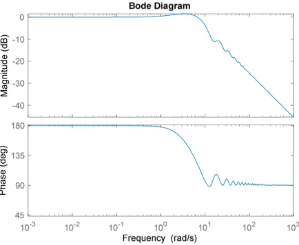
Figure 4.1 Bode Diagram of &'() (1st Order Case) After that, bound for 𝛾 is calculated as [0, 10] from

[ 𝛾𝑙𝑜𝑤𝑒𝑟 = 𝑚𝑎𝑥|W(zeros of M(s))| , 𝛾𝑢𝑝𝑝𝑒𝑟 = ||W||∞ ]

On the other hand, by performing very small increase rate on the bound of 𝛾, 𝐷_𝐺 = 𝛾2− 𝑊∗𝑊 = 0 is implemented and 𝛽_𝑘′𝑠 are obtained every time. Then, 𝛽_𝑘 values are substituted to 𝑁_𝐺 one by one in order to obtain 𝑅𝛾.

25

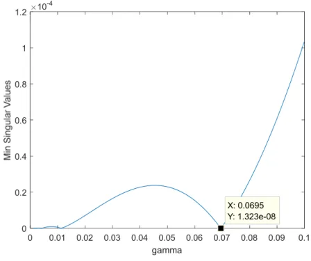
𝑁𝐺(𝛽𝑘) = 0 is the 𝑘𝑡ℎ _{equation, which is defined as (8), in 𝑅𝛾𝛿 = 0. So,} 𝑅𝛾 is computed at every step and singular value decomposition is applied on it to compute singular vector 𝛿, 𝛾_𝑜𝑝𝑡 is the largest 𝛾 for which 𝑅_𝛾 is singular. Following figure illustrates this process:

Figure 4.2 Minimum Singular Values of 𝑅_𝛾 versus 𝛾 (1st Order Case) Therefore, 𝛾_𝑜𝑝𝑡 equal to 0.312 and corresponding 𝛽_𝑘 values are {3.2036j, −3.2036j}. After that, the singular vector 𝛿 is obtained as follow-ing:

𝛿 = [𝜙1

𝜃1]=[−0.1936−0.9811]

With this result, 𝐺(𝑠) can be easily found since 𝛿 and 𝛾_𝑜𝑝𝑡 help us to find 𝑁𝐺 and 𝐷𝐺 respectively. After finding 𝐺(𝑠), 𝑄𝑜𝑝𝑡(𝑠) can be found since 𝑄𝑜𝑝𝑡 = 𝛱+𝑀

∗_𝑊𝐺

𝐺 . Results for 𝐺(𝑠) and 𝑄𝑜𝑝𝑡 are obtained in state – space form and Bode plots for both of them provided:

0.05 0.1 0.15 0.2 0.25 0.3 0.35 0.4 gamma 0 0.01 0.02 0.03 0.04 0.05 0.06 0.07 X: 0.312 Y: 5.796e-06

26

Figure 4.3 Bode plot for 𝐺(𝑠) (1st Order Case)

Figure 4.4 Bode plot for 𝑄𝑜𝑝𝑡 (1st Order Case)

We have no clue about the structure of 𝑄𝑜𝑝𝑡 up to now, since we do not perform hand calculation and we obtained the results in state – space form.

M a g n it u d e ( d B ) P h a s e ( d e g ) M a g n it u d e ( d B ) P h a s e ( d e g )

27

Thereafter, we will try to find the structure of 𝑄𝑜𝑝𝑡. We know that the general form of 𝑄_𝑜𝑝𝑡 is 𝑄_𝑜𝑝𝑡 = 𝛾𝑜𝑝𝑡𝑄𝐹

1+𝑄𝐹𝐻𝑜𝑝𝑡−𝐹𝐼𝑅. It is straightforward to obtain

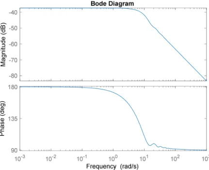
𝐻𝑜𝑝𝑡(𝑠) by taking inverse of 𝑄𝑜𝑝𝑡. Then we have 𝐻𝑜𝑝𝑡(𝑠) in the state – space form. The Bode plot of it is provided as at below:

Figure 4.5 Bode plot for 𝐻_𝑜𝑝𝑡 (1st Order Case)

At this point, what should be done is obtaining the delay – free part of 𝐻𝑜𝑝𝑡(𝑠). From the procedure indicated and mentioned in Chapter 3, delay – free part of 𝐻𝑜𝑝𝑡(𝑠) is computed as:

𝐻𝑜𝑝𝑡−𝑑𝑒𝑙𝑎𝑦𝑓𝑟𝑒𝑒(𝑠) = −2.0846 ∗ 10

−8 _{(s − 9.594 ∗ 10}6_{) (s − 51.26)} (𝑠2 _{+ 10.26)}

≅ 0.2 (s − 51.26)_{(𝑠2 + 10.26)}

As can be seen from above result, 𝐻𝑜𝑝𝑡−𝑑𝑒𝑙𝑎𝑦𝑓𝑟𝑒𝑒(𝑠) has poles which are exactly equal to 𝛽_𝑘 values. In this manner, 𝑄₂ = 0 which gives us following equalities for this example:

M a g n it u d e ( d B ) P h a se ( d e g )

28

𝐻𝑜𝑝𝑡−𝐹𝑖𝑙𝑡𝑒𝑟(𝑠) = 𝐻𝑜𝑝𝑡−𝑑𝑒𝑙𝑎𝑦𝑓𝑟𝑒𝑒(𝑠) 𝐻𝑜𝑝𝑡(𝑠) = 𝐻𝑜𝑝𝑡−𝐹𝐼𝑅(𝑠)

𝑄𝐹 = 1

By simply converting 𝐻_{𝑜𝑝𝑡−𝐹𝑖𝑙𝑡𝑒𝑟}(𝑠) to state – state form we obtain A, B and C as state – space matrices of 𝐻_{𝑜𝑝𝑡_𝐹𝐼𝑅}(𝑠). The rest is implementing the following:

𝐻𝑜𝑝𝑡−𝐹𝐼𝑅(𝑠) = 𝐶(𝑠𝐼 − 𝐴)−1_{𝐵 − 𝐶𝑒}𝐴ℎ_𝑒−ℎ𝑠_{(𝑠𝐼 − 𝐴)}−1_𝐵

As stated in previous part, 𝐻_{𝑜𝑝𝑡−𝐹𝐼𝑅}(𝑠) is put into process as two separate parts, which are 𝐶(𝑠𝐼 − 𝐴)−1𝐵 and 𝐶𝑒𝐴ℎ𝑒−ℎ𝑠(𝑠𝐼 − 𝐴)−1𝐵.

Obviously, 𝐶(𝑠𝐼 − 𝐴)−1𝐵 part indicates the delay – free part of 𝐻𝑜𝑝𝑡−𝐹𝐼𝑅(𝑠), which is the filter 𝐻𝑜𝑝𝑡−𝐹𝑖𝑙𝑡𝑒𝑟(𝑠) itself. From 𝐶𝑒𝐴ℎ_𝑒−ℎ𝑠_{(𝑠𝐼 −} 𝐴)−1_{𝐵 part we obtain the delay part of 𝐻}

𝑜𝑝𝑡−𝐹𝐼𝑅(𝑠) which is the

𝐻𝑜𝑝𝑡−𝑑𝑒𝑙𝑎𝑦(𝑠). Therefore, we separately get all parts of 𝐻𝑜𝑝𝑡−𝐹𝐼𝑅(𝑠). This

result is sufficient to reveal 𝐻_{𝑜𝑝𝑡−𝐹𝐼𝑅}(𝑠)’s and also 𝐻_𝑜𝑝𝑡(𝑠)’s structure in this example: 𝐻𝑜𝑝𝑡−𝑑𝑒𝑙𝑎𝑦(𝑠) = −3.2051 (s + 0.1007)𝑒 −0.5𝑠 (𝑠2 _{+ 10.26)} ≅ −3.2051 (s + 0.1)𝑒 −0.5𝑠 (𝑠2 _{+ 10.26)} 𝐻𝑜𝑝𝑡(𝑠) = 𝐻𝑜𝑝𝑡−𝑑𝑒𝑙𝑎𝑦𝑓𝑟𝑒𝑒(𝑠) − 𝐻𝑜𝑝𝑡−𝑑𝑒𝑙𝑎𝑦(𝑠) 𝐻𝑜𝑝𝑡(𝑠) = 𝑄2+ 𝐻𝑜𝑝𝑡−𝐹𝑖𝑙𝑡𝑒𝑟(𝑠) − 𝐻𝑜𝑝𝑡−𝑑𝑒𝑙𝑎𝑦(𝑠) 𝐻𝑜𝑝𝑡(𝑠) = 𝐻𝑜𝑝𝑡−𝐹𝐼𝑅(𝑠) = 𝐻𝑜𝑝𝑡−𝐹𝑖𝑙𝑡𝑒𝑟(𝑠) − 𝐻𝑜𝑝𝑡−𝑑𝑒𝑙𝑎𝑦(𝑠) => 𝐻𝑜𝑝𝑡(𝑠) = 𝐻𝑜𝑝𝑡−𝐹𝐼𝑅(𝑠) = 0.2 (s − 51.26) + 3.2051 (s + 0.1)𝑒 −0.5𝑠 (𝑠2 _{+ 10.26)}

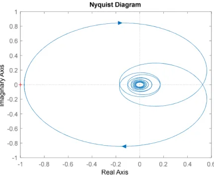
Although the denominator expression of 𝐻_𝑜𝑝𝑡(𝑠) has roots on the imagi-nary axis, these get cancelled by the zeros of the numerator, which are the 𝛽𝑘 values, exactly at the same points. Thereby, 𝐻𝑜𝑝𝑡(𝑠) is stable which en-sures the stability of 𝑄_𝑜𝑝𝑡(𝑠). The stability of 𝑄_𝑜𝑝𝑡(𝑠) can be observed from the Nyquist plot of 𝐻_𝑜𝑝𝑡(𝑠). As can be seen at the figure below, there is no

29

encirclement around s = -1 since there is no pole at the right half plane as at below:

Figure 4.6 Nyquist plot of 𝐻_𝑜𝑝𝑡(𝑠) (1st Order Case)

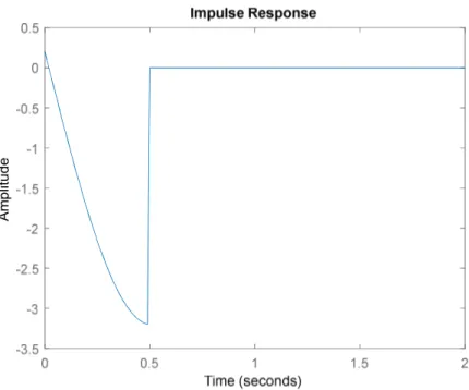
On the other hand, impulse response of ℎ(𝑡) is observed as expected since ℎ(𝑡) is FIR. It can be seen at the following figure:

Im a g in a ry A x is

30

Figure 4.7 Impulse Response for ℎ(𝑡) (1st Order Case)

This result completes the general structure searching for 𝑄_𝑜𝑝𝑡(𝑠) since we have already determined the general form of 𝑄_𝑜𝑝𝑡(𝑠) as 𝑄_𝑜𝑝𝑡 = 𝛾𝑜𝑝𝑡

1+𝐻𝑜𝑝𝑡 =

𝛾𝑜𝑝𝑡𝑄𝐹

1+𝑄_𝐹𝐻_{𝑜𝑝𝑡−𝐹𝐼𝑅}. In this manner, the structural result for 𝑄𝑜𝑝𝑡 in this example

comes forward as following:

𝑄𝑜𝑝𝑡 =_{1 + 𝑄𝐹}𝛾𝑜𝑝𝑡_{𝐻𝑜𝑝𝑡−𝐹𝐼𝑅}𝑄𝐹 =_{1 + 𝐻}𝛾𝑜𝑝𝑡 𝑜𝑝𝑡−𝐹𝐼𝑅 = 0.312 1 + (0.2 (s − 51.26) + 3.2051 (s + 0.1)𝑒_(𝑠2 _{+ 10.26)} −0.5𝑠) ∎ This example can be considered main example with detailed explanations. Following examples will be given as only resultative and also used as check-sum of our computation method for different types of 𝑊(𝑠).

A m p lit u d e

31

4.2

Second Order Weight

𝐖

Let 𝑊(𝑠) =_{(𝑠+0.1)(𝑠+0.05)}1 𝜖 𝐻_∞ and 𝑀(𝑠) = 𝑒−0.5𝑠 𝜖 𝐻_∞. Bode plot for 𝑊(𝑠) is the following:

Figure 4.8 Bode Diagram of 𝑊(𝑠) (2nd Order Case)

Then, from [ 𝛾_{𝑙𝑜𝑤𝑒𝑟}= 𝑚𝑎𝑥|W(zeros of M(s))| , 𝛾_{𝑢𝑝𝑝𝑒𝑟} = ||W||_∞ ] bound for 𝛾 is calculated as [0, 200]

Again, by performing very small increase rate on the bound of 𝛾, 𝑅_𝛾 is computed at every step and singular value decomposition is applied on it, 𝛾𝑜𝑝𝑡 is the largest 𝛾 for which 𝑅𝛾 is singular. This procedure is illustrated at the following figure:

-300 -200 -100 0 100 W(s) (Example 1) W(s) (Example 2) 10-6 10-4 10-2 100 102 104 106 -180 -135 -90 -45 0 Bode Diagram Frequency (rad/s)

32

Figure 4.9 Minimum Singular Values versus 𝛾 (2nd Order Case) Thus, 𝛾_𝑜𝑝𝑡 is equal to 0.0695 and corresponding 𝛽_𝑘 values are {3.7943, 3.7926j, −3.7943, −3.7926j}. Then, the singular vector 𝛿 are ob-tained as following: 𝛿 = ⎣ ⎢⎢ ⎡𝜙_𝜙1₂ 𝜃1 𝜃2⎦ ⎥⎥ ⎤ = ⎣ ⎢⎡ −0.0130 −0.0133 −0.4447 −0.8955⎦⎥⎤

With 𝛾𝑜𝑝𝑡 and 𝛿 vector, 𝐺(𝑠) and 𝑄𝑜𝑝𝑡(𝑠) are obtained in state – space form, again. The Bode plots for both of them are at below:

0 0.01 0.02 0.03 0.04 0.05 0.06 0.07 0.08 0.09 0.1 gamma 0 0.2 0.4 0.6 0.8 1 1.2 10 -4 X: 0.0695 Y: 1.323e-08

33

Figure 4.10 Bode plot for 𝐺(𝑠) (2nd Order Case)

Figure 4.11 Bode plot for 𝑄_𝑜𝑝𝑡(𝑠) (2nd Order Case)

M a g n it u d e ( d B ) P h a se ( d e g ) M a g n it u d e ( d B ) P h a se ( d e g )

34

From here, we can easily obtain 𝐻𝑜𝑝𝑡(𝑠) by taking inverse of 𝑄𝑜𝑝𝑡 and have 𝐻_𝑜𝑝𝑡(𝑠) in the state – space form. The Bode plot of 𝐻_𝑜𝑝𝑡(𝑠) is given at following figure:

Figure 4.12 Bode plot for 𝐻_𝑜𝑝𝑡 (2nd Order Case)

As in the first example, the delay – free part of 𝐻_𝑜𝑝𝑡(𝑠) is computed as: 𝐻𝑜𝑝𝑡−𝑑𝑒𝑙𝑎𝑦𝑓𝑟𝑒𝑒(𝑠) ≅ −5.376 (s − 3.989) (s + 2.234) (𝑠_{(s − 3.794) (s + 3.794) (s + 2.838) (𝑠}2 + 1.905s + 12.26)_{2+ 14.38)}

As obvious, the expression of 𝐻𝑜𝑝𝑡−𝑑𝑒𝑙𝑎𝑦𝑓𝑟𝑒𝑒(𝑠) has poles exactly at 𝛽𝑘 values. There is also an additional negative pole which comes from 𝑄₂. In order to obtain 𝐻_{𝑜𝑝𝑡−𝐹𝑖𝑙𝑡𝑒𝑟}(𝑠), we should find 𝑄₂(𝑠) from the residues of

𝐻𝑜𝑝𝑡−𝑑𝑒𝑙𝑎𝑦𝑓𝑟𝑒𝑒(𝑠) and substract it from 𝐻𝑜𝑝𝑡−𝑑𝑒𝑙𝑎𝑦𝑓𝑟𝑒𝑒(𝑠) equation.

Hence, 𝑄2(𝑠) = 2.3242_{s + 2.838} M a g n it u d e ( d B ) P h a se ( d e g )

35 From 𝑄_𝐹 =_1+𝑄1

2 we have:

𝑄𝐹 = s + 2.838_{s + 5.162}

Then, by executing 𝐻_{𝑜𝑝𝑡−𝐹𝑖𝑙𝑡𝑒𝑟}(𝑠) = 𝐻_{𝑜𝑝𝑡−𝑑𝑒𝑙𝑎𝑦𝑓𝑟𝑒𝑒}(𝑠) − 𝑄₂(𝑠), we get:

𝐻𝑜𝑝𝑡−𝐹𝑖𝑙𝑡𝑒𝑟(𝑠) = −7.003 (s − 3.928)(𝑠

2 _{+ 1.195s + 12.45)}

(s − 3.794) (s + 3.794)(𝑠2_{+ 14.38)}

After converting 𝐻_{𝑜𝑝𝑡−𝐹𝑖𝑙𝑡𝑒𝑟}(𝑠) to state – space form, we get A, B and C state – space matrices to calculate 𝐻_{𝑜𝑝𝑡−𝑑𝑒𝑙𝑎𝑦}(𝑠) and 𝐻_{𝑜𝑝𝑡−𝐹𝐼𝑅}(𝑠). With the same implementation on first example, 𝐻_{𝑜𝑝𝑡−𝑑𝑒𝑙𝑎𝑦}(𝑠) is computed as:

𝐻𝑜𝑝𝑡−𝑑𝑒𝑙𝑎𝑦(𝑠) = 3.1581 ∗ 10 −11 _{(s + 4.557 ∗ 10}11_{)(s + 0.1)(s + 0.05) 𝑒}−0.5𝑠 (s − 3.794)(s + 3.794)(𝑠2 _{+ 4.565 ∗ 10}−13_{+ 14.38)} ≅ 14.39 (s + 0.1)(s + 0.05) 𝑒_{(s − 3.794)(s + 3.794)(𝑠2+ 14.38)}−0.5𝑠 Then, 𝐻𝑜𝑝𝑡−𝐹𝐼𝑅(𝑠) = 𝐻𝑜𝑝𝑡−𝐹𝑖𝑙𝑡𝑒𝑟(𝑠) − 𝐻𝑜𝑝𝑡−𝑑𝑒𝑙𝑎𝑦(𝑠) = −7.003 (s − 3.928)(𝑠2_{(s − 3.794)(s + 3.794)(𝑠} + 1.195s + 12.45) − 14.39 (s + 0.1)(s + 0.05) 𝑒_{2+ 14.38)} −0.5𝑠 Thus, 𝐻𝑜𝑝𝑡(𝑠) = 𝑄2(𝑠) + 𝐻𝑜𝑝𝑡−𝐹𝐼𝑅(𝑠) 𝐻𝑜𝑝𝑡(𝑠) = 2.3242 (s + 2.838) (−7.003 (s − 3.928)(𝑠 2 _{+ 1.195s + 12.45) − 14.39 (s + 0.1)(s + 0.05) 𝑒}−0.5𝑠 (s − 3.794)(s + 3.794)(𝑠2_{+ 14.38)} )

Here, the denominator expression of 𝐻_𝑜𝑝𝑡(𝑠) has roots on the imaginary axis and the right-half plane. These get cancelled by the zeros of the numer-ator, which are the 𝛽_𝑘 values, exactly at the same points. On the other hand, 𝑄2(𝑠) is both proper and stable transfer function. Thereby, 𝐻𝑜𝑝𝑡(𝑠) is stable

36

which ensures the stability of 𝑄𝑜𝑝𝑡(𝑠). The stability of 𝑄𝑜𝑝𝑡(𝑠) can be ob-served from the Nyquist plot of 𝐻_𝑜𝑝𝑡(𝑠):

Figure 4.13 Nyquist plot of 𝐻_𝑜𝑝𝑡(𝑠) (2nd Order Case)

37

As can be seen at the figures above, there is no encirclement around s = -1, since there is no unstable pole.

Also, the impulse response of ℎ(𝑡) is observed as FIR which can be seen at figure below:

Figure 4.15 Impulse Response for ℎ(𝑡) (2nd Order Case)

This result completes the general structure searching for 𝑄𝑜𝑝𝑡(𝑠) since we know the form of 𝑄_𝑜𝑝𝑡(𝑠) as 𝑄_𝑜𝑝𝑡 = 𝛾𝑜𝑝𝑡𝑄𝐹

1+𝑄_𝐹𝐻_{𝑜𝑝𝑡−𝐹𝐼𝑅}. Hence, the structural

re-sult of 𝑄𝑜𝑝𝑡 for this example is computed as at below: 𝑄𝑜𝑝𝑡 =_{1 + 𝑄}𝛾𝑜𝑝𝑡𝑄𝐹

𝐹𝐻𝑜𝑝𝑡−𝐹𝐼𝑅

= 0.0695 (s + 2.838s + 5.162)

1 + (s + 2.838_{s + 5.162) (}−7.003 (s − 3.928)(𝑠₍2_{s − 3.} + 1.195s + 12.45_{794)(s + 3.794)(})− 14.39 _𝑠2_{+ 14.}(₃₈s + 0.1) )(s + 0.05) 𝑒−0.5𝑠)

38

4.3

Third Order Weight

𝐖

Let 𝑊(𝑠) =_{(𝑠+0.1)(𝑠+0.05)(𝑠+10)}1 𝜖 𝐻_∞ and 𝑀(𝑠) = 𝑒−0.5𝑠 𝜖 𝐻_∞. Relative Bode plots for 𝑊(𝑠) are given in the following figure:

Figure 4.16 Bode Diagram of 𝑊(𝑠) (3rd Order Case)

From [ 𝛾𝑙𝑜𝑤𝑒𝑟 = 𝑚𝑎𝑥|W(zeros of M(s))| , 𝛾𝑢𝑝𝑝𝑒𝑟 = ||W||∞ ] bound for 𝛾 is calculated as [0, 20]

As before, by performing very small increase rate on the bound of 𝛾, 𝑅𝛾 is computed at every step and singular value decomposition is applied on it. This procedure is illustrated at the following figure:

M a g n it u d e ( d B ) P h a se ( d e g )

39

Figure 4.17 Minimum Singular Values versus 𝛾 (3rd Order Case) Thus, 𝛾_𝑜𝑝𝑡 equal to 0.0046756 and corresponding 𝛽_𝑘 values are {9.7428, 4.9644, 4.422j, −9.7428, − 4.9644, −4.422j}. Then, the singular vec-tor 𝛿 are obtained as following:

𝛿 = ⎣ ⎢ ⎢ ⎢ ⎢ ⎡𝜙1_𝜙2 𝜙3 𝜃1 𝜃2 𝜃3⎦ ⎥ ⎥ ⎥ ⎥ ⎤ = ⎣ ⎢⎢ ⎢ ⎡0.12870.0051 0.1311 0 0.4357 0.8811⎦ ⎥⎥ ⎥ ⎤

With 𝛾_𝑜𝑝𝑡 and 𝛿 vector, 𝐺(𝑠) and 𝑄_𝑜𝑝𝑡(𝑠) are obtained in state – space form. The Bode plots for both of them are at below:

M in S in g u la r V a lu e s

40

Figure 4.18 Bode plot for 𝐺(𝑠) (3rd Order Case)

Figure 4.19 Bode plot for 𝑄_𝑜𝑝𝑡(𝑠) (3rd Order Case)

M a g n it u d e ( d B ) P h a se ( d e g ) M a g n it u d e ( d B ) P h a se ( d e g )

41

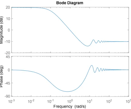
In here, we can obtain 𝐻𝑜𝑝𝑡(𝑠) by taking inverse of 𝑄𝑜𝑝𝑡 and have 𝐻𝑜𝑝𝑡(𝑠) in the state – space form. The Bode plot of 𝐻_𝑜𝑝𝑡(𝑠) is given at following figure:

Figure 4.20 Bode plot for 𝐻_𝑜𝑝𝑡 (3rd Order Case)

As in the first example, the delay – free part of 𝐻_𝑜𝑝𝑡(𝑠) is computed as:

𝐻𝑜𝑝𝑡−𝑑𝑒𝑙𝑎𝑦𝑓𝑟𝑒𝑒(𝑠) = −6.6902 (𝑠 + 2.831)(𝑠 − 5.267)(𝑠 − 9.701)(𝑠 + 9.907)(𝑠 + 10.48)(𝑠2 _{+ 1.899𝑠 + 16.54)} (s + 9.78)(s + 9.743)(s + 4.964)(s + 3.715)(s − 4.964)(s − 9.743)(𝑠2 _{+ 2.259 ∗ 10}−13_{s + 19.56)} 𝐻𝑜𝑝𝑡−𝑑𝑒𝑙𝑎𝑦𝑓𝑟𝑒𝑒(𝑠) ≅ −6.6902 (𝑠 + 2.831) (𝑠 − 5.267) (𝑠 − 9.701) (𝑠 + 9.907) (𝑠 + 10.48) (𝑠2 + 1.899𝑠 + 16.54) (s + 9.78)(s + 3.715) (s + 9.743)(s − 9.743)(s + 4.964) (s − 4.964)(𝑠2 _{+ 19.56)}

Here, the expression of 𝐻_{𝑜𝑝𝑡−𝑑𝑒𝑙𝑎𝑦𝑓𝑟𝑒𝑒}(𝑠) has poles exactly at 𝛽_𝑘 values. There are also additional negative poles which come from 𝑄2(𝑠). In order to obtain 𝐻_{𝑜𝑝𝑡−𝐹𝑖𝑙𝑡𝑒𝑟}(𝑠), we should find 𝑄₂(𝑠) from the residues of 𝐻𝑜𝑝𝑡−𝑑𝑒𝑙𝑎𝑦𝑓𝑟𝑒𝑒(𝑠) and substract it from 𝐻𝑜𝑝𝑡−𝑑𝑒𝑙𝑎𝑦𝑓𝑟𝑒𝑒(𝑠) equation.

M a g n it u d e ( d B ) P h a se ( d e g )