Seabed propagation of ULF/ELF electromagnetic fields from harmonic dipole sources located on the seafloor

Radio Science, Volume 23, Number 6, Pages 931-943, November-December 1988

Seabed propagation of ULF/ELF electromagnetic fields from harmonic dipole sources

located on the seafloor

A. C. Fraser-Smith, x A. S. lnan, 2 0. G. Villard, Jr., x and R. G. Joiner 3 (Received February 29, 1988; accepted May 11, 1988.)

The amplitudes of the quasi-static electromagnetic fields generated at points on the seafloor by harmonic dipole sources (vertically directed magnetic dipoles, horizontally directed magnetic dipoles,

vertically

directed

electric

dipoles,

and horizontally

directed

electric

dipoles)

also

located

on the sea-

floor are computed using a numerical integration technique. The primary purpose of these compu- tations is to obtain field amplitudes that can be used in undersea communication studies. An important secondary purpose is to examine the enhancements of the fields produced at moderate to large dis- tances by the presence of the relatively less conducting seafloor, as compared with the fields produced at the same distances in a sea of infinite extent, for frequencies in the ULF/ELF bands (frequencies less than 3 kHz). These latter enhancements can be surprisingly large, with increases of 4 orders of mag- nitude or more being typical at distances of 20 seawater skin depths.

1. INTRODUCTION

Because of the high attenuation involved (55 dB/

wavelength), communication through seawater by means of freely propagating electromagnetic waves is difficult to accomplish and is usually restricted to frequencies in the lowest part of the radio band, where the wavelengths are largest, and to ranges that are short in comparison to those that can be achieved at the same frequencies above the sea sur- face. While it does not yet appear possible to avoid

this high attenuation when the transmitter and

receiver are both deeply immersed and separated from interfaces with other media by many seawater skin depths, a number of studies have suggested that increased range can be achieved by locating the sub-

merged transmitter and receiver near to the sea sur- face and utilizing the "up-over-and-down," or "sur-

face," mode of propagation [e.g., Moore and Blair,

1961; Hansen, 1963; Moore, 1967; Bubenik and

Fraser-Smith, 1978]. In this mode the major part of the propagation path is through air, a low-loss

medium, and increased range results. Less well known is the "down-under-and-up," or "seabed," •Space, Telecommunications, and Radioscience Laboratory, Stanford University, Stanford, California.

•-Department of Electrical and Electronics Engineering, Bilkent University, Ankara.

3Office of Naval Research, Arlington, Virginia. Copyright 1988 by the American Geophysical Union. Paper number 8S0356.

0048-6604/88/008S-0356508.00

mode of propagation [Mott and Biggs, 1963; Coggon and Morrison, 1970; Frieman and Kroll, 1973; Bostick et al., 1978; Bubenik and Fraser-Smith, 1978; lnan, 1984; King et al., 1986; King, 1986; lnan et al., 1986]. The seabed, being electrically conducting, has nom- inally the same 55 dB/wavelength rate of attenuation

for propagating electromagnetic fields as does seawa-

ter, but because its electrical conductivity is less, and

possibly much less, than that of seawater, the wave- length is larger and the attenuation per unit distance

is smaller. Some of the properties of this mode were studied by Bubenik and Fraser-Smith [1978] for a

transmitter and receiver located at points equidistant between the surface and floor of a sea one seawater skin depth deep. We now extend this earlier work by

considering specifically the increased propagation range that might be achieved by placing the trans-

mitter and receiver directly on the seafloor and making full use of the seabed mode. As we will show,

substantial increases in range can result.

This work is essentially a continuation of a recent

study, reported by lnan et al. [1986], on the enhance-

ments and other changes produced in the ULF/ELF fields generated along the seafloor by long current- carrying cables also located on the seafloor. Also rel- evant is the article by Fraser-Smith et al. [1987] de-

scribing large amplitude changes in dipole fields in-

duced by the seabed under different circumstances

from those investigated here.

Until the last few years it was difficult to evaluate many of the expressions for the field components

produced along a seafloor by harmonic dipole 931

932 FRASER-SMITH ET AL.: SEABED PROPAGATION OF ELECTROMAGNETIC FIELDS

sources located on the seafloor without either making major simplifying assumptions, and thus ob- taining approximate (sometimes very approximate) values for the field components, or being forced to use numerical integration techniques, which can be difficult to implement but which can give accurate field values over wide ranges of frequency and dis-

tance.

Our approach

to computing

dipole

fields

has

been to use a numerical integration technique, and that is the method we have used in this work to obtain the field values. However, a substantial ana- lytical advance has recently been made by R. W. P. King and his coworkers in evaluating the fields pro- duced along a seafloor, with the result that a number of new analytical expressions of varying degrees of approximation are now available for the field com- ponents [e.g., King and Brown, 1984; King, 1985a, b]. We find that there is good agreement between the

field values we compute and the field values com- puted from King's least approximate expressions

within their ranges of applicability. We also find good agreement, in fact agreement to many signifi- cant figures, between field values we compute using our numerical integration technique and field values calculated from the exact analytical expressions for certain field components produced by vertical mag- netic and horizontal electric dipole sources [Wait,

1952, 19613.

The seabed in our work is represented by a single

semi-infinite conducting layer, and thus no attempt is made to take account of the lithospheric duct mode of propagation, concerning which there now exists a considerable literature [e.g., Wait, 1954; Wheeler, 1961; Burrows, 1963; Gabillard et al., 1971; Wait and Spies, 1972a, b, c; Heacock, 1971; Bostick et al.,

1978]. If such a duct does exist, as suggested by the

literature (but unfortunately not yet adequately

tested by experiment), there should be increases in the amplitudes of the electromagnetic fields produced

at the receiver above those predicted by our compu- tations. However, because our transmitter and receiv- er are located on the seafloor, and therefore some

distance above the probable center of the duct, the

increase in the field levels is much more likely to be due to a lower effective seabed conductivity than to any ducting of fields.

Although we refer to the seabed "mode of propa-

gation" in this work, we should point out that the

mode is not a clearly defined theoretical entity as are,

for example, the transverse magnetic, transverse elec-

tric, and transverse electromagnetic modes in wave-

guides. We use the term to distinguish the fields propagating primarily through the seabed from those propagating (1) directly through the sea ("direct mode"), (2) in the up-over-and-down mode ("surface

mode"), or (3) in a variety of higher-order modes. It

is possible to separate the contributions of the

various modes to the net fields measured at the

receiver, as is done by Bubenik and Fraser-Smith [1978] and King [1985a]. However, by choosing a very deep sea and a transmitter and receiver located on the seafloor, as is done here, we eliminate the up-over-and-down and higher-order modes and minimize the contribution from the direct mode.

This work has application in studies of the proper- ties of the seabed and its electrical conductivity in particular (see Bannister [1968] and Coggon and Mor-

rison [1970] for earlier work on this topic). It also qualifies as a study of seabed effects in general [e.g.,

Weaver, 1967 ; Ramaswamy et al., 1972]. However, we believe its primary application is in undersea com-

munication. This application appears promising for

the following reasons. First, as we will show in this

paper, the seabed propagation mode offers ranges

that may be large in comparison with those that can be achieved directly through seawater. Second, the ambient noise level on the seafloor is likely to be much lower than at the sea surface. Third, unlike

other possible undersea transmitter-receiver configu-

rations, once a transmitter and receiver have been

installed on the seafloor, their positions are unlikely to change in the long term, and they can be com-

paratively easily located again for maintenance, if

necessary. Finally, it would be possible to colocate a chain of receiver-transmitter pairs (analogous to the

repeaters used in other communication links) on the seafloor between the primary transmitter and receiv-

er and thus achieve increased range.

2. CALCULATION OF FIELD COMPONENTS

Figure 1 shows the geometry employed in the cal-

culation of the electromagnetic field components pro-

duced at points on the seafloor by harmonic dipole sources also located on the seafloor. A cylindrical coordinate system (r, •b, z) is used, and the dipoles, of moment m (magnetic dipoles) or p (electric dipoles) and angular frequency co (co = 2rrf), are placed at the

origin with the vertical dipole moments directed

upward along the z axis and with the horizontal

dipole moments directed along the x axis (•b = 0).

The seafloor is the plane z = 0, the region z > 0 is

FRASER-SMITH ET AL.: SEABED PROPAGATION OF ELECTROMAGNETIC FIELDS 933

tivity as), and the region z < 0 is the seabed,

which is

assumed

to be a homogeneous

conducting

half-space

with permittivity

es, permeability

tto, and conduc-

tivity af. The field components

are computed

at

points

P(r, •p, 0). We consider

all major categories

of

dipole sources:

vertically

directed

electric

and mag-

netic dipoles (VEDs and VMDs, respectively)

and

horizontally

directed

electric

and magnetic

dipoles

(HEDs and HMDs, respectively).

The field ex-

pressions

for the four dipole types are as follows:

1. Vertical electric dipole

Er- P F2•i;,

2 d2

(1)

Ez p fo

-

©

-- F•M

1

23 d2

(2)

#O

P

fo•

1

B

• -•

u

•

iW#o

rn

•o

©

1 2

2

E't' •

u•

Pøm

•o

© 2

2

B

r = •

F2e dX

(5)

•o

mfo

©

1 •3

d•

(6)

B• •

u•

VED

•

r Ez

//t

__

B•

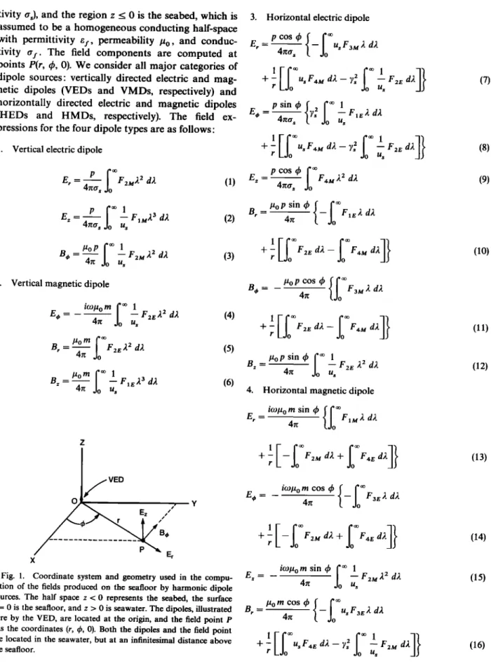
Fig. 1. Coordinate system and geometry used in the compu- tation of the fields produced on the sea floor by harmonic dipole

sources. The half space z < 0 represents the seabed, the surface z = 0 is the seafloor, and z > 0 is seawater. The dipoles, illustrated here by the VED, are located at the origin, and the field point P

has the coordinates (r, •p, 0). Both the dipoles and the field point are located in the seawater, but at an infinitesimal distance above

the seafloor.

3. Horizontal electric dipole

E

r pcøs

- 4•% - UsF3M2

•P

{ fo•

d2

1[;o•

fo

•1 1}

p cos

•p F,•M

22

d2

Br •

#0

P

sin

•p

{;o

©

F•e

2 d2

1

[foøø fo

© ]}

©

B,

= --/•o

P

cos

•b F3M

2 d2

1

[foøø •o

© 1}

B• #oP

sin

•p

fo

©

1

4. Horizontal magnetic dipole

irø#omsinrP{fo•

imPornCøsqb{

fo•

1

[ foø• •o

© ]}

ic%u

o

m

sin

•p

fo

©

1

Br

=

/'tøm

4rr

cøs

½P

{ foø•

-- us

F3•r/]'

d2

1[;o•

fo

•1

934 FRASER-SMITH ET AL.: SEABED PROPAGATION OF ELECTROMAGNETIC FIELDS

B•

=

#øm

4•t 7s -- F•M

sin

• f 2•o•

1

'• d2

1[•o•

[o

•1 1t

©

B•

= Pøm

cos

• F4e2

a d2

(18)

All the above field quantities are sinusoidal func- tions of time, and thus, in the representation used

here, they are complex quantities with the implicit

multiplier e •', and the actual fields are given by the

pressions: where (20a) (200) (21) (22)

Here #o is the permeability of free space (#o

x 10-7 H/m; the seabed

is assumed

to be nonmag-

netic), and the quantities

7s and 7f are the propaga-

tion constants for the sea and seabed. There is an

approximation involved in the two expressions that

are given for Vs and •.. For a general

conducting

72 = --c02#• + ico#• (23)

but for the conducting media and frequencies of in-

terest in this work (ULF/ELF; frequencies less than

3 kHz) the displacement

current

term co2#e

may be

space wavelength [Kraichman, 1976]. This condition is always well satisfied for the source receiver dis- tances considered in this paper, and thus our data

could be said to apply under the conditions of the quasi-static approximation. However, the terminol- ogy appears to have little significance when the prop- agation paths are confined to conducting media.

We evaluated the dipole field expressions numeri-

cally, using the techniques described by Bubenik

[1977]. The dipole moments were set equal to unity

(m= 1 A m 2 and p=l

A m), and for dipoles of

field magnitudes. The computations were also carried

out in normalized form, to preserve generality and to

reduce the computational effort [Bubenik and Fraser- Smith, 1978; Fraser-Smith and Bubenik, 1979, 1980].

The two important features of this normalization are

(1) the seabed conductivity is referred to that of sea- water, and (2) distances are measured in units of the

seawater skin depth 6•, where

6 s -- (2/601aoO's) TM (24)

As a result of this normalization procedure, fre-

quency and conductivity are removed as explicit variables during evaluation of the field expressions. We use the picotesla as our unit for the magnetic

field (1 pT = 1 m• = 10-•2 T), and the electric

field

data are presented in units of microvolts per meter.

3. NUMERICAL RESULTS

Our results consist of amplitude data for (1) the radial and vertical electric field components E, and

E z, the total electric field Exo

x, and the total mag-

netic field Bxox (Bxox

= B•,) produced

by the VED,

E•), and the total magnetic

field component

Bxox

E•, E•), three

magnetic

field components

(B•, B•, B•),

field data; furthermore, as we will now show, it does

not significantly limit the applicability of the field data at general azimuthal angles.

Because of the sin 4• and cos 4• terms appearing in the equations for the field components produced by

FRASER-SMITH ET AL.: SEABED PROPAGATION OF ELECTROMAGNETIC FIELDS 935

the two horizontal dipoles (equations (7)-(18)), only

one of the horizontal

electric

components

(E r and E,)

and Be) are produced

by each of the dipoles

when

•b = 0 ø or 90 ø (these nonzero horizontal components

are denoted either by E.o R and B.o R, when there is a

vertical electric or magnetic field component present

as well, or by EToT or BTo x, when they are the only

electric or magnetic field component; whether they are radial or azimuthal can be determined quickly by noting the azimuthal angle and referring to (7)-(18)).

Similarly, only one of the two vertical components E z and B z is produced at each of the two azimuthal angles. As a result, only three basic electric and mag-

netic field components are produced by the horizon- tal dipoles when •b = 0 ø and 90 ø. These two choices of 4• therefore simplify the presentation of numerical field data, but not at the expense of generality, since

field amplitudes at an arbitrary 4• can be obtained by

multiplying the amplitudes given for (p = 0 ø or 4• = 90 ø by the appropriate value of cos 4• or sin 4•. The choice of which angular function to use is deter- mined by the presence of the function in the appli- cable equation of the set (7)-(18). For example, sup-

pose amplitudes are required for the three electric

field components

E•, Ee, and Ez produced

by the

E• are found by referring to the HED, 4• = 0 ø, results

and multiplying the appropriate values of E.o R and E z by cos 4•, which appears in (7) and (9) for the two

field components,

and the amplitude

of Ee is found

plying the appropriate Exo x value by sin (p, which

appears in (8).

The presentation of the field data is similar, but not identical, to presentations used previously by Bu-

benik and Fraser-Smith [1978] and Fraser-Smith and Bubenik [1979, 1980]. First, we present a series of curves that give, in this case, the actual amplitudes of

the fields produced on the seafloor by a particular unit moment dipole that is also located on the sea- floor. Next, we present additional curves that give the ratios of the amplitudes of the fields produced by the dipole in the presence of the seabed to the ampli-

tudes produced under otherwise identical conditions

by the dipole submerged in the sea of infinite depth. These latter curves enable us to identify the changes produced in the fields specifically by the presence of

the seabed, since the absence of a seabed effect is indicated by a ratio of unity.

To further illustrate the effects produced on the

field quantities by the seabed, the normalized seabed

conductivity

af/as is varied widely, with values

in the

range 1 (no seabed effect), 0.3, 0.1, 0.03, 0.01, 0.003, 0.001. It is possible that some materials in a real seabed have a normalized conductivity less than 0.001, but it is unlikely that the effective overall con- ductivity will be less than 0.001, because of the in-

clusion of the relatively high conductivity sediments close to the floor. Studies of the seafloor conductivity

[e.g., Young and Cox, 1981] suggest that a typical conductivity for the first 1 km of the seabed is 0.1 S/m. Thus the range of seabed conductivities con- sidered in our computations should cover most prac-

tical seabeds.

The field data are presented in six figures, as fol-

lows: VED, Figure 2; VMD, Figure 3; HED, 4> = 0ø, Figure 4; HED, •b = 90 ø, Figure 5; HMD, •b = 0 ø, Figure 6; and HMD, 4• = 90 ø, Figure 7. Within each

figure, there are four panels on the left providing the field amplitudes in parametric form, and matching panels on the right containing the curves showing the ratios of the field amplitudes produced by the dipole

on the seafloor to the amplitudes produced under otherwise identical conditions but with the seabed

replaced

by seawater

(aœ

- as). The ratio curves

pro-

vide an immediate qualitative indication of the scale of the enhancements, or decreases, of the field ampli- tudes due to the presence of the seabed, since, as we have noted, the absence of a seabed effect is indicated by a ratio of 1.0 (in the figures, this corresponds to a horizontal line passing through 0 on the vertical axis). In addition, if desired, the curves can be used to

give quantitative information about the changes in

the fields caused by the seabed.

To provide an example of the use of the data in Figures 2-7, suppose the source of the fields is a

VED of moment 10 A m transmitting at 100 Hz and

we wish to know the amplitude of E z at a distance of

r = 100 m on a seabed with an effective conductivity

of O. la s. First, we compute the seawater skin depth

6s at 100 Hz (it will be assumed

that a s --4.0 S/m)

panel for E• in Figure 2 we read off E• x 6•3as

= 3.0

x 102 ktV/m x m2S, or E• -- 0.0047 #V/m. This elec-

tric field amplitude applies to a unit moment dipole;

for a dipole of moment 10 A m it is Ez - 0.047 #V/m.

Turning to the ratio curveS, we make the perhaps surprising finding that the seabed reduces the ampli-

tude of E• to about 0.35 of its equivalent value in seawater of infinite extent; it is only for distances greater than 106 s in this example that the amplitude

FRASER-SMITH ET AL.' SEABED PROPAGATION OF ELECTROMAGNETIC FIELDS 937

[(uoo'• vas ON) XO X:4 /(U00'• vaS H.UnO XO X:4 ]0 • •)O9

[(aaa vas ON) xoxs/(aaa vas H].I?•) ].O.I.s]0[•)O1

ON) z•/(aaa vas H.LI•) z•]o[•)O"l

c• •'g o

938

FRASER-SMITH

ET AL.' SEABED

PROPAGATION

OF ELECTROMAGNETIC

FIELDS

.,-,.

• l- HED,

4,:O':'

,r]

/

.

...

, ...

•6• X

-•

•

03

3

i

LOG10

HOF!IZONTAL

DISTANCE

r/•s

LOG•0

HORIZONTAL

DISTANCE

r/•

s

Fig.

4. Variation

with

distance

along

the

seafloor

of the

amplitudes

of the

electromagnetic

fields

produced

at an

azimuthal

angle

• of 0 ø by a horizontally

directed

harmonic

electric

dipole

(left).

The

amplitudes

are

shown

for

seabed

conductivities

oz in the

range

0.•1• to 1.0•, where

• is the

conductivity

of the

seawater.

Also

shown

(right)

are

ratio

cur•es

illustrating

the

contribution

made

by

the

seabed

to the

field

amplitudes

shown

in the

panels

on the left.

begins

to show

an increase

due to the presence

of the

seabed,

but the increase

with increasing

distance

then

becomes

very rapid.

Finally,

if we divide

the ampli-

tude of E z (0.047

#V/m) for the unit moment

dipole

by 0.35,

we obtain

a numerical

value

for the ampli-

tude (0.134

#V/m) that would be produced

by the

dipole

in a sea

of infinite

extent.

The same

amplitude

can be computed from the appropriate field ex-

pression

in the set given by Kraichrnan

[1976] for

dipoles

immersed

in an infinite

conducting

medium,

thus providing a check of the results of our numerical

computations.

For each dipole category there is at least one and

sometimes

two (HED, •b = 0ø; and HMD, •b = 0 ø)

matching

panels missing

on the right-hand

sides of

the displays.

The reason

for the gaps

is of great

in-

terest

from the point of view of the effects

produced

by a seabed.

Not only can the seabed

change

the

amplitudes

of the field components

that would be

present

in the absence

of the bed

(a

s = as)

, but it can

also produce

new field components

which, in addi-

tion, often have amplitudes

that are greater

than

those

of the other

components

at large

distances.

Be-

cause

these

latter components

do not exist in a sea of

infinite

extent,

ratio curves

cannot

be computed,

and

gaps

are produced

in the displays.

The missing

panels

on the right-hand

sides

of the figures

therefore

pro-

vide a guide to the field quantities

that owe their

existence

to the presence

of the seabed.

To be specif-

FRASER-SMITH ET AL.: SEABED PROPAGATION OF ELECTROMAGNETIC FIELDS 939

ON) -LO-L3/(aaa •s HIIM) -I-O-I-::!]0[ OO' j

[(aaa vas ON) .Lo. Le/(aaa vas n.un0 xoxe]or•)Oq

½

ø

(•w

• w/^•)

[see•,

• .LO.L3]OI.

DO-

!

(gw

• J.d)

•, • zE!]oI.

DO'I

i :• øø

_ß

_•

•

_o

ß

••o.•

940 FRASER-SMITH ET AL.: SEABED PROPAGATION OF ELECTROMAGNETIC FIELDS

_

:i HMD,

••

z• !

of/as

=

0.001

@ -

_

m •

... ... ,x

,x,

... ... ...

o•os

=

0.•1

0

I

2

1

0

1

2

-1 ... I ... I ...

LOG10 HORIZONTAL DISTANCE r/6s LOG•0 HORIZONTAL DISTANCE r/6s

Fi•. 6. Variation

with

distance

alon•

the

scafioo•

o[ the

amplitudes

o[ the

electromagnetic

fidds

p•oduccd

at an

(fi•ht)

a•c

•atio

curves

illustratin•

the

contribution

o• the

seabed

to the

field

amplitudes

shown

in the

pands

on the

HED, •b = 0 ø, Ez and B, (or BTOT);

HED, •b = 90

ø, B,.

(or Bi•oR);

HMD, •b = 0 ø, E, (or ETOT)

and Bz; and

HMD, •b = 90 ø, E,. (or Ei•oR

). In addition to the miss-

ing ratio panels for these components,

it will be

noted that the parametric

amplitudes

are only plot-

ted for o'f/o'

s _<

0.3, since the components

do not

exist

for as/as = 1.

For comparison with our dipole field data we also

computed numerical values for some of the field components produced by an HED located on the

seafloor

using

the approximate

expressions

given

by

pressions

for the HED electric

field

component

given by King [1985a, equations

(10b) and (45a)] and

conductivities

and distances.

The most approximate

expression,

given by King's equation

(10b), gives

field

amplitudes

differing

from ours and from those

given

by King's more accurate

expression

(equation

(45a))

by up to a factor of 2, depending

on which part of

King's "useful intermediate range" is involved. On

the other hand, the more accurate

expression

gives

field values that are in close agreement

with ours,

particularly

within the middle part of the range of

In addition to the above comparison, we also com-

puted values

of E, and B• for the VMD and B• for

the HED using

exact analytical

expressions

given

by

those

obtained

by our numerical

integration

method.

FRASER-SMITH ET AL.' SEABED PROPAGATION OF ELECTROMAGNETIC FIELDS 941

[(O511] ¾:JS ON) J-OJ-:l/(Oal] ¾:JS HJ. IM) J.OJ.:l]01.•)O- j [(O511] ¾:JS ON) Z:lj'(Oal] ¾:JS HJ. IM) Z:l]Ol'•)O-J •

... I ... I ... I ... I: ... [(Q:•I] V-dS ON) J.OJ.j•/(a:•l] V-dS HJ. IM) J.OJ.j•]01. •)O-J

z

942 FRASER-SMITH ET AL.: SEABED PROPAGATION OF ELECTROMAGNETIC FIELDS

For the distances and seabed conductivities covered by the data in Figures 2-7 there was excellent agree- ment between the two sets of field data, usually to many significant figures. However, for combinations of large distances and high seabed conductivities out- side those illustrated in the figures, the field quan- tities became so small that computer rounding errors

in the numerical integration method introduced dis- crepancies. Partly for this reason, and partly to save

computation time, the ratio data in the figures were computed using the known analytical expressions for

the fields produced in a sea of infinite depth [Kraich-

man, 1976].

4. DISCUSSION

There are a number of interesting general features

of the data shown in Figures 2-7. First, as antici- pated, there can be substantial increases in the field components produced along the seafloor in compari-

son to those that would be produced under otherwise identical conditions in a sea of infinite extent. These increases only occur for horizontal distances greater

than about 36 s, but they then grow rapidly with dis-

tance. Increases of 4 orders of magnitude or more at

distances of 206s are typical. Second, for field ampli- tudes that are approaching the limit of detection of present measurement systems, the presence of the seabed can increase the range of detection of the fields by roughly 2-10 times, depending on the ef- fective conductivity of the seabed. Third, as we have already noted, additional field components are pro- duced when a seabed is present (in comparison to a sea of infinite depth), and some of these additional components predominate at larger distances. Finally, fourth, the ratio curves tend to be very similar for the range of seabed conductivities covered by our com-

putations

(as/a.•

= 0.001-0.3 S/m). Nevertheless,

we

passing

through 0 on the vertical axis as as/a.•--o

1,

and there is indeed some evidence for this transfor-

mation when the ratio curves

for as/a s = 0.1 and 0.3

this result is that the field amplitudes produced at

distances greater than about 5•s are particularly sen- sitive to seabed conductivities in the range 0.1as to 1.Oas. Conversely, except for the VED fields and E z for the HMD, •p = 90 ø, the field amplitudes tend not to be very sensitive to seabed conductivities less than about 0.1as.

Comparing the fields generated along the seafloor,

we see that there are some major differences between

dipole types. In particular, for low seabed conduc-

tivities, the HED and HMD produce much larger

fields at large distances than do the VED and VMD.

The difference is substantial, amounting to 2 orders

of magnitude

at a distance

of 1006, for as/a., - 0.001.

This result is in agreement with the more restricted observation by Friernan and Kroll [1973] that an

HED was far superior to a VED for producing ULF fields along the seafloor. We might also comment that the VED also appears inferior to other dipole types for producing fields at short to moderate dis- tances (r < 106.,), particularly when the seabed has a

low effective conductivity.

In conclusion, this study makes evident the impor-

tant role that the seafloor could play in undersea

communication by means of freely propagating ULF/ELF electromagnetic waves from harmonic dipole sources located on or near the seafloor. The

combination of possible large seabed enhancements

of the fields, comparatively low noise levels from at- mospheric sources, and a fixed surface on which re- peaters can be located could well make feasible the utilization of the seabed as a communication

medium.

Acknowledgments. We thank D. M. Bubenik for the use of his computer code and P. R. Bannister for helpful discussions. This work was supported by the Office of Naval Research under con-

tract N00014-83-K-0390.

REFERENCES

Bannister, P. R., Determination of the electrical conductivity of the sea bed in shallow waters, Geophysics, 33, 995-1003, 1968.

Bostick, F. X., C. S. Cox, and E. C. Field, Jr., Land-to-seafloor

electromagnetic transmissions in the 0.1 to 15 Hz band, Radio

$ci., 13, 701-708, 1978.

Bubenik, D. M., A practical method for the numerical evaluation of Sommerfeld integrals, IEEE Trans. Antennas Propeg., AP-25,

904-906, 1977.

Bubenik, D. M., and A. C. Fraser-Smith, ULF/ELF electro-

magnetic fields generated in a sea of finite depth by a sub- merged vertically-directed harmonic magnetic dipole, Radio Sci.,

13, 1011-1020, 1978.

Burrows, C. R., Radio communication within the Earth's crust, IEEE Trans. Antennas Propag., AP-25, 311-317, 1963.

Coggon, J. H., and H. F. Morrison, Electromagnetic investigation of the sea floor, Geophysics, 35, 476489, 1970.

Fraser-Smith, A. C., and D. M. Bubenik, ULF/ELF electro- magnetic fields generated above a sea of finite depth by a sub- merged vertically-directed harmonic magnetic dipole, Radio $ci.,

14, 59-74, 1979.

Fraser-Smith, A. C., and D. M. Bubenik, Compendium of the ULF/ELF electromagnetic fields generated above a sea of finite depth by submerged harmonic dipoles, Tech. Rep. E715-1, 114 pp., Radiosci. Lab., Stanford Univ., Stanford, Calif., 1980.

FRASER-SMITH ET AL.: SEABED PROPAGATION OF ELECTROMAGNETIC FIELDS 943

Fraser-Smith, A. C., D. M. Bubenik, and O. G. Villard, Jr., Large- amplitude changes induced by a seabed in the sub-LF electro- magnetic fields produced in, on, and above the sea by harmonic dipole sources, Radio Sci., 22, 567-577, 1987.

Frieman, E. A., and N.M. Kroll, Lithospheric propagation for undersea communication, Tech. Rep. JSR-73-5, 23 pp., Stanford

Res. Inst., Menlo Park, Calif., 1973.

Gabillard, R., P. Degauque, and J. R. Wait, Subsurface electro- magnetic telecommunication--A review, IEEE Trans. Commun.

Technol., COM-19, 1217-1228, 1971.

Hansen, R. C., Radiation and reception with buried and sub- merged antennas, IEEE Trans. Antennas Propag., AP-11, 207-

216, 1963.

Heacock, J. G. (Ed.), The Structure and Physical Properties of the

Earth's Crust, Geophys. Monogr. Ser., vol. 14, 348 pp., AGU, Washington, D.C., 1971.

Inan, A. S., Propagation of electromagnetic fields along the sea/sea-bed interface, Tech. Rep. E721-2, 70 pp., Space, Tele-

commun. and Radiosci. Lab., Stanford Univ., Stanford, Calif.,

1984.

Inan, A. S., A. C. Fraser-Smith, and O. G. Villard, Jr., ULF/ELF

electromagnetic fields generated along the seafloor interface by a straight current source of infinite length, Radio Sci., 21, 409-

420, 1986.

King, R. W. P., Electromagnetic surface waves: New formulas and applications, IEEE Trans. Antennas Propag., AP-33, 1204-1212,

1985a.

King, R. W. P., Electromagnetic surface waves: New formulas and their application to determine the electrical properties of the sea

bottom, J. Appl. Phys., 58, 3612-3624, 1985b.

King, R. W. P., Properties of the lateral electromagnetic field of a vertical dipole and their application, IEEE Trans. Geosci.

Remote Sens., GE-24, 813-825, 1986.

King, R. W. P., and M. F. Brown, Lateral electromagnetic waves along plane boundaries: A summarizing approach, Proc. IEEE,

72, 595-611, 1984.

King, R. W. P., M. Owens, and T. T. Wu, Properties of lateral electromagnetic fields and their application, Radio Sci., 21,

13-23, 1986.

Kraichman, M. B., Handbook of Electromagnetic Propagation in

Conducting Media, U.S. Government Printing Office, Wash- ington, D.C., 1976.

Moore, R. K., Radio communication in the sea, IEEE Spectrum, 4, 42-51, 1967.

Moore, R. K., and W. E. Blair, Dipole radiation in a conducting half-space, J. Res. Natl. Bur. Stand., Sect. D, 65, 547-563, 1961. Mott, H., and A. W. Biggs, Very-low-frequency propagation below

the bottom of the sea, IEEE Trans. Antennas Propag., AP-11, 323-329, 1963.

Ramaswamy, V., H. W. Dosso, and J. T. Weaver, Horizontal mag-

netic dipole embedded in a two-layer conducting medium, Can.

J. Phys., 50, 607-616, 1972.

Wait, J. R., Current-carrying wire loops in a simple inhomoge- neous region, J. Appl. Phys., 23, 497-498, 1952.

Wait, J. R., On anomalous propagation of radio waves in earth

strata, Geophysics, 19, 342-343, 1954.

Wait, J. R., The electromagnetic fields of a horizontal dipole in the presence of a conducting half-space, Can. J. Phys., 39, 1017-

1028, 1961.

Wait, J. R., and K. P. Spies, Electromagnetic propagation in an idealized earth crust waveguide, I, Pure Appl. Geophys., 101,

174-187, 1972a.

Wait, J. R., and K. P. Spies, Electromagnetic propagation in an idealized earth crust waveguide, II, Pure Appl. Geophys., 101,

188-193, 1972b.

Wait, J. R., and K. P. Spies, Dipole excitation of ultra-low- frequency electromagnetic waves in the earth crust waveguide, J. Geophys. Res., 77, 7118-7120, 1972c.

Weaver, J. T., The quasi-static field of an electric dipole embedded

in a two-layer conducting half-space, Can. J. Phys., 45, 1981- 2002, 1967.

Wheeler, H. A., Radio-wave propagation in the earth's crust, J. Res. Natl. Bur. Stand., Sect. D, 65, 189-191, 1961.

Young, P. D., and C. S. Cox, Electromagnetic active source sounding near the East Pacific Rise, Geophys. Res. Lett., 8,

1043-1046, 1981.

A. C. Fraser-Smith and O. G. Viilard, Jr., STAR Laboratory,

Stanford University, Stanford, CA 94305.

A. S. Inan, Department of Electrical and Electronics Engineer- ing, Bilkent University, Ankara, Turkey.