Graph problems in call models and switching networks

GRAPH PROBLEMS IN CALL MODELS

AND SWITCHING NETWORKS

a dissertation submitted to

the graduate school of engineering and science

of bilkent university

in partial fulfillment of the requirements for

the degree of

doctor of philosophy

in

computer engineering

By

Abdullah Atmaca

August 2018

GRAPH PROBLEMS IN CALL MODELS AND SWITCHING NETWORKS

By Abdullah Atmaca August 2018

We certify that we have read this dissertation and that in our opinion it is fully adequate, in scope and in quality, as a dissertation for the degree of Doctor of Philosophy.

Cevdet Aykanat(Advisor)

A. Yavuz Oru¸c(Co-Advisor)

U˘gur G¨ud¨ukbay

Can Alkan

Engin Demir

Tayfun K¨u¸c¨ukyılmaz Approved for the Graduate School of Engineering and Science:

Ezhan Kara¸san

ABSTRACT

GRAPH PROBLEMS IN CALL MODELS AND

SWITCHING NETWORKS

Abdullah Atmaca

Ph.D. in Computer Engineering Advisor: Cevdet Aykanat Co-Advisor: A. Yavuz Oru¸c

August 2018

In the first part of this dissertation, we focus on graph problems that arise in call models. Such models are used to study the combinatorial properties of certain types of calls that include unicast, multicast, and bicast interconnections. Here we focus on bicast calls, and provide closed-form expressions for the number of unlabeled bicast calls when either the number of callers or number of receivers is fixed to 2 or 3. We then obtain lower and upper bounds on the number of such calls by solving an open problem in graph theory, namely counting the number of unlabeled bipartite graphs. Next, these results are extended to left (right) set labeled and set labeled bipartite graphs. In the second part of the dissertation, we focus on wiring and routing problems for one-sided, binary tree switching networks. Specifically, we reduce the O(n) time complexity of the routing algorithm for the one-sided, binary tree switching networks to O(lg n). We also present a new wiring algorithm for one-sided, binary tree switching networks. Finally, an algorithm is presented to locate the cluster in which the terminals of the corresponding one-sided binary tree switching network are paired. The time complexity of this algorithm is shown to be O(lg n).

Keywords: Bipartite graphs, Polya’s counting theorem, cycle index polynomial, switching networks, call models.

¨

OZET

C

¸ A ˘

GRI MODELLER˙I VE ANAHTARLAMA

A ˘

GLARINDA C

¸ ˙IZGE PROBLEMLER˙I

Abdullah Atmaca

Bilgisayar M¨uhendisli˘gi, Doktora Tez Danı¸smanı: Cevdet Aykanat ˙Ikinci Tez Danı¸smanı: A. Yavuz Oru¸c

A˘gustos 2018

Bu tezin ilk b¨ol¨um¨unde, ¸ca˘grı modellerinde ortaya ¸cıkan ¸cizge problemlerine odaklanılmaktadır. Bu t¨ur modeller, tekli ¸ca˘grı, ¸coklu ¸ca˘grı ve kar¸sılıklı ¸coklu ¸ca˘grı ba˘glantılarını i¸ceren bazı ¸ca˘grı tiplerinin kombinatoryel ¨ozelliklerini incele-mek i¸cin kullanılır. Burada, kar¸sılıklı ¸coklu ¸ca˘grılara odaklanıyoruz ve arayan-ların sayısı veya alıcıarayan-ların sayısı 2 veya 3’e sabitlendi˘ginde etiketsiz kar¸sılıklı ¸coklu ¸ca˘grıların sayısı i¸cin kapalı form ifadeleri sa˘glıyoruz. Bu durumda, ¸cizge teorisinde a¸cık bir problemi ¸c¨ozerek, yani etiketsiz iki par¸calı ¸cizgeleri sayarak bu t¨ur ¸ca˘grıların sayısıyla ilgili alt ve ¨ust sınırlar elde ediyoruz. Daha sonra, bu sonu¸clar, sol(sa˘g) tarafı k¨ume olarak etiketli ve iki tarafı da k¨ume olarak etiketli iki par¸calı ¸cizgelere geni¸sletilmektedir. Tezin ikinci b¨ol¨um¨unde, tek taraflı, ikili a˘ga¸c anahtarlama a˘gları i¸cin ba˘glama ve y¨onlendirme problemlerine odak-lanıyoruz. ¨Ozellikle, tek taraflı, ikili a˘ga¸c anahtarlama a˘gları i¸cin y¨onlendirme algoritmasının O(n) hesaplama zamanını O(lg n)’e d¨u¸s¨ur¨uyoruz. Tek taraflı, ikili a˘ga¸c anahtarlama a˘gları i¸cin yeni bir ba˘glama algoritması da sunuyoruz. Son olarak, ba˘glama tasarımı verilen tek taraflı, ikili a˘ga¸c anahtarlama a˘gının termi-nallerinin e¸sle¸stirildi˘gi k¨umenin yerini belirlemek i¸cin bir algoritma sunulmu¸stur. Bu algoritmanın zaman karma¸sıklı˘gının O(lg n) oldu˘gu g¨osterilmi¸stir.

Anahtar s¨ozc¨ukler : ˙Iki par¸calı ¸cizgeler, Polya sayma teoremi, d¨ong¨u endeks poli-nomu, anahtarlama a˘gları, ¸ca˘grı modelleri.

Acknowledgement

I would like to express my gratitude to Prof. Dr. Cevdet Aykanat and Prof. Dr. A. Yavuz Oru¸c, from whom I have learned a lot, due to their supervision, suggestions, and support during this research.

I am also indebted to Prof. Dr. U˘gur G¨ud¨ukbay, Asst. Prof. Dr. Can Alkan, Asst. Prof. Dr. Engin Demir and Asst. Prof. Dr. Tayfun K¨u¸c¨ukyılmaz for showing keen interest to the subject matter and accepting to read and review this thesis.

I would like to thank the Scientific and Technological Research Council of Turkey (T ¨UB˙ITAK) for its financial support.

Finally, I would like to thank my family, especially my wife, for the continuous support they have given me throughout writing this thesis.

Contents

1 Introduction 1

2 Counting Two Families of Unlabeled Bipartite Graphs 4

2.1 Preliminary Facts . . . 4

2.2 A Closed-Form Expression for _|Bu(2, r)| . . . 8

2.3 A Closed-Form Expression for |Bu(3, r)| . . . 11

2.4 An Elementary Counting for _|Bu(2, r)| . . . 17

3 Bounds for Unlabeled Bipartite Graphs 20 3.1 A Lower Bound for |Bu(n, r)| . . . 20

3.2 An Upper Bound for _|Bu(n, r)| . . . 23

4 Labeled Bipartite Graphs 37 4.1 Preliminary Facts . . . 37

4.2 Left-Set-Labeled Bipartite Graphs . . . 38

4.2.1 Counting Left-Set-Labeled Bipartite Graphs . . . 38

4.2.2 A Lower Bound for _|Bx(n, r)| . . . 42

4.2.3 Upper Bounds for |Bx(n, r)| . . . 44

4.3 Set-Labeled Bipartite Graphs . . . 45

4.3.1 Counting Set-Labeled Bipartite Graphs . . . 46

4.3.2 Bounds for Set-Labeled Bipartite Graphs . . . 48

5 Two Problems in Network Wiring and Switching 51 5.1 Motivation . . . 51

5.2 Routing in One-Sided, Binary Tree Switches . . . 51

CONTENTS vii

5.4 The Routing Algorithm . . . 56

6 Concluding Remarks 58

6.1 Future Work . . . 58

Bibliography 60

Appendices 64

A Implementation of Proposed Wiring Method 64

B Implementation of Proposed Routing Method 66

C Complete Implementation of Proposed Wiring and Routing

Method 67

List of Figures

2.1 Unlabeled bipartite graphs for n = 3 and r = 2 . . . 5 2.2 Construction of unlabeled (2, r)-bipartite graphs with exactly two

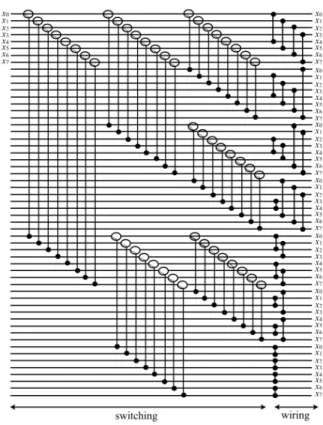
left vertices, 1_{ i  r. . . .} 18 5.1 An 8 terminal, one-sided switch wiring. . . 57

List of Tables

3.1 Exact values of ln_|Bu(n, r)|, 1  n < r  15, and natural

List of Symbols

Bu(n, r) The set of unlabeled bipartite graphs with n left and r right vertices.

Sn The symmetric group of permutations of degree n.

ZSn The cycle index polynomial of Sn.

Bx(n, r) The set of all left-set-labeled bipartite graphs with n left and r right

vertices.

Bx(n, r, i) The set of (n, r)-left-set-labeled bipartite graphs in each of which the

degrees of exactly i left vertices are greater than 0.

Bx(n, r) The set of all (n, r)-unlabeled bipartite graphs in each of which the

degrees of all left vertices are greater than 0. Bxy(n, r) The set of all (n, r)-set-labeled bipartite graphs.

Bxy(i, j) The set of all (i, j)-unlabeled bipartite graphs such that there is no

Chapter 1

Introduction

This dissertation is concerned with the solutions of certain graph problems in com-binatorial call models and switching networks. Switching networks have beeen extensively investigated in connection with communication systems, and multi-processing and parallel computing [1–18]. Our work is motivated by the recent renewed interest in such call models and networks due to the introduction of on-chip systems, especially network-on-on-chip architectures. In particular, one-sided switching networks were reported in [19] as a possible network architecture for an on-chip network. Two problems were introduced in this connection to reduce the area/volume complexity of the targeted on-chip network. One deals with wiring replicates of terminals that represent cores, while the other is concerned with routing connection requests. Even though some solutions were provided for both of these problems in [19–21], these solutions place a restriction on the num-ber of terminals in the case of wiring, and an exact excessive time complexity in the case of routing. Both these issues have been addressed in this dissertation and resolved. On the other hand, call models have been introduced in [19] to classify switching networks. E↵ectively, they capture the multiplicities of calls and ordering of callers and/or receivers under various call scenarios. Each of these call models can be represented by a bipartite graph with certain conditions. Broadly speaking, three call models distinguish between the multiplicity proper-ties of calls, and three more conditions are added to each of these call models

to characterize the ordering between the callers and receivers. A comprehensive description of these di↵erent call models can be found in [19]. The enumeration of calls leads to the crosspoint complexity of switching networks that can realize the set of calls defined by such call models using a logarithmic transformation. One problem that has been highlighted in [19] is the enumeration of the corre-sponding bipartite graphs that represent the call models of interest. A number of formulas have been provided in [19], but the enumerations of bipartite graphs in some of the call models have not been concluded with asymptotic closed-form formulas. One of the main contributions of this dissertation is to settle this prob-lem. More specifically, we provide both exact and asymptotic formulas that count the number of bipartite graphs in the aforementioned call models; in particular for unlabeled bicast, left(right) set labeled and set labeled bicast calls.

The contributions of this dissertation are stated below:

1. An exact closed-form expression for the number of unlabeled bipartite graphs one of whose parts consists of two vertices.

2. An exact closed-form expression for the number of unlabeled bipartite graphs one of whose parts consists of three vertices.

3. The solution of the long-standing open problem that was stated in 1973 [22]. Specifically, a lower bound on the number of unlabeled bipartite graphs, and an upper bound within a factor of two of the lower bound have been established using Polya’s Counting Theorem.

4. The results in (1), (2), and (3) have been extended to left (right) set labeled and set labeled bipartite graphs.

5. The O(n) time complexity of the routing algorithm given in [20] for the one-sided, binary tree switching network has been reduced to O(lg n). 6. A new wiring algorithm has been given for one-sided, binary tree switching

7. An algorithm has been presented to locate the cluster in which the terminals of the corresponding one-sided, binary tree switching network are paired. The time complexity of this algorithm is O(lg n).

The rest of this dissertation is organized as follows. In Chapters 2 and 3, enu-merations of unlabeled bipartite graphs are considered. We give exact results for the size of two families of unlabeled bipartite graphs in Chapter 2 and derive lower and upper bounds on the number of unlabeled bipartite graphs in Chap-ter 3. We extend these calculations to left set labeled and set labeled bipartite graphs in Chapter 4. In Chapter 5, we reduce the time complexity of a routing method in one-sided switching network. We also introduce a new wiring method to cluster replicates of cores into clusters and provide a new routing algorithm for this wiring architect. Finally, we conclude the dissertation in Chapter 6. The appendix lists computer programs that implement the proposed algorithms and provides some sample results.

Chapter 2

Counting Two Families of

Unlabeled Bipartite Graphs

In this chapter, we present two results that provide the exact number of distinct unlabeled bipartite graphs when the cardinality of one of the sets of vertices is fixed to 2 or 3.

2.1

Preliminary Facts

This problem has been investigated in connection with the enumeration of unla-beled bipartite graphs and binary matrices [22]. Our work has been motivated in part by a counting problem that arises in the representation of calls in inter-connection networks [19]. Let (I, O, E) denote a graph with two disjoint sets of vertices, I, called left vertices and a set of vertices, O, called right vertices, where each edge in E connects a left vertex with a right vertex. We let n =|I|, r = |O|, and refer to such a graph as an (n, r)-bipartite graph. Let G1 = (I, O, E1) and

G2 = (I, O, E2) be two (n, r)-bipartite graphs, and ↵ : I ! I and : O ! O be

both bijections. The pair (↵, ) is an isomorphism between G1 and G2 provided

1

that ((↵(v1), (v2))2 E2 if and only if (v1, v2)2 E1, 8v1 2 I, 8v2 2 O. It is easy

to establish that this mapping induces an equivalence relation, and partitions the set of 2nr _{(n, r)-bipartite graphs into equivalence classes. This equivalence}

relation captures the fact that the vertices in I and O are unlabeled, and so each class of (n, r)-bipartite graphs can be represented by any one of the graphs in that class without identifying the vertices in I and O. Let Bu(n, r) denote any

set of (n, r)-bipartite graphs that contains exactly one such graph from each of the equivalence classes of (n, r)-bipartite graphs induced by the isomorphism we defined. It is easy to see that determining _|Bu(n, r)| amounts to an

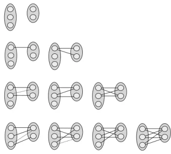
enumera-tion of non-isomorphic (n, r)-bipartite graphs that will henceforth be referred to as unlabeled (n, r)-bipartite graphs. Figure 2.1 depicts the unlabeled bipartite graphs for n = 3 and r = 2.

Figure 2.1: Unlabeled bipartite graphs for n = 3 and r = 2

In [22], Harrison used P´olya’s counting theorem to obtain an expression to com-pute the number of non-equivalent n⇥r binary matrices. This expression contains a nested sum, in which one sum is carried over all partitions of n while the other is carried over all partitions of r, where the argument of the nested sum involves factorial, exponentiation and greatest common divisor (gcd) computations. He further established that this formula also enumerates the number of unlabeled (n, r)-bipartite graphs. A number of results indirectly related to Harrison’s work

appeared in the literature [23–26]. In particular, the set Bu(n, r) in our work

coincides with the set of bicolored graphs described in Section 2 in [23]. Whereas Harary [23] provides a counting polynomial for the number of bicolored graphs, we focus on the asymptotic behavior of _|Bu(n, r)|. Counting polynomials for other

families of bipartite graphs were also reported in [24]. Likewise, Hanlon [25], and Gainer-Dewar and Gessel [26] provide generating functions for related bi-partite graph counting problems without an asymptotic analysis as provided in our contributions. The species and category theory approach in [26] leads to a summation formula for the number of unlabeled bipartite graphs with v vertices. This formula is similar to the expression in (8) in [22] except that the latter for-mula counts the number of unlabeled bipartite graphs whose vertices are divided into two disjoint sets as in the model that we used in our research. As such, for fixed n and r, the set Bu(n, r) forms a subset of the set of unlabeled bipartite

graphs with v vertices that are counted in [25,26], where v = n + r. It should also be mentioned that some results on asymptotic enumeration of certain families of bipartite graphs (binary matrices) have been reported (see for example, [27–30]). That_|Bu(1, r)| = r+1 trivially holds. Exact closed form expressions for |Bu(n, r)|

for n = 2, n = 3, and any integer r > n will be given in the remaining of this chapter.

Let Sn denote the symmetric group of permutations of degree n acting on set

N = _{{1, 2, · · · , n}. Suppose that the n! permutations in S}n are indexed by

1, 2,· · · , n! in some arbitrary, but fixed manner. The cycle index polynomial of Sn is defined as follows([31], see p. 35, Eqn. 2.2.1):

ZSn(x1, x2,· · · , xn) = 1 n! n! X m=1 n Y k=1 xpm,k k (2.1)

where pm,k denotes the number of cycles of length k in the disjoint cycle

repre-sentation of the mth _{permutation in S}

Let Sn⇥ Sr denote the direct product of symmetric groups Sn and Sr acting on

N ={1, 2, · · · , n} and R = {1, 2, · · · , r}, respectively, where n and r are positive integers such that n < r. It can be inferred from Harrison ([32], Lemma 4.1 and Theorem 4.2) that the cycle index polynomial of Sn⇥ Sr is given by

ZSn⇥Sr(x1, x2,· · · , xnr) = ZSn(x1, x2,· · · , xn)⇥ ZSr(x1, x2,· · · , xr), (2.2)

where ⇥ is a particular polynomial multiplication that distributes over ordinary addition, and in which the multiplication XmJXt of two product terms, Xm=

xpm,1 1 x pm,2 2 · · · x pm,n n and Xt = xq1t,1x qt,2 2 · · · x qt,r r in ZSn and ZSr, respectively, is defined as Xm K Xt = n Y k=1 r Y j=1 xpm,kqt,jgcd(k,j) lcm(k,j) . (2.3)

Note that we will not display the zero powers of x1, x2,· · · in a cycle index

poly-nomial. We will use the same convention for all other cycle index polynomials throughout the thesis. The lcm(a,b) and gcd(a,b) denote least common multiple and greatest common divisor of a and b.

Harrison further proved that [22]:

|Bu(n, r)| = ZSn⇥Sr(2, 2, .., 2 | {z }

nr

) (2.4)

when n_{6= r. As noted in [22], n = r case involves a di↵erent cycle index} polyno-mial and will be omitted here as well.

We need one more fact that can be found in Harary ([31], p. 36) in order to compute_|Bu(2, r)| and |Bu(3, r)|: ZSr(x1, x2, . . . , xr) = 1 r r X i=1 xiZSr i(x1, x2, . . . , xr i) (2.5) where ZS0() = 1.

2.2

A Closed-Form Expression for

_|B

(2, r)

|

We use Polya’s counting theorem (See [33]), in particular Harrison’s cycle index formulation in [22] to compute_|Bu(2, r)|. We calculate _|Bu(2, r)| as follows: |Bu(2, r)| = ZS2⇥Sr(2, 2, . . . , 2), (2.6) = [ZS2(x1, x2)⇥ ZSr(x1, x2, . . . , xr)] (2, . . . , 2), (2.7) = ✓ 1 2 x 2 1+ x2 ◆ ⇥ ZSr(x1, x2, . . . , xr) (2, . . . , 2), (2.8) =1 2 ⇥ x2₁⇥ ZSr(x1, x2, . . . , xr) + x2⇥ ZSr(x1, x2, . . . , xr) ⇤ (2, . . . , 2), (2.9) =1 2 (_h x2₁⇥ 1 r! r! X t=1 r Y j=1 xqt,j j i (2, . . . , 2) +hx2⇥ 1 r! r! X t=1 r Y j=1 xqt,j j i (2, . . .), ) , (2.10) =1 2 ( h 1 r! r! X t=1 x2₁K r Y j=1 xqt,j j i (2, . . . , 2) +h 1 r! r! X t=1 x2 K_Yr j=1 xqt,j j i (. . .) ) , (2.11) =1 2 ( h 1 r! r! X t=1 r Y j=1 x2qt,jgcd(1,j) lcm(1,j) i (2, . . . , 2) +h 1 r! r! X t=1 r Y j=1 xqt,jgcd(2,j) lcm(2,j) i (. . .). ) , (2.12) =1 2 ( h 1 r! r! X t=1 r Y j=1 x2qt,j j i (2, . . . , 2) +h 1 r! r! X t=1 r Y j=1 xqt,jgcd(2,j) lcm(2,j) i (2, . . . , 2) ) , (2.13) =1 2 ( h 1 r! r! X t=1 r Y j=1 22qt,j i +h 1 r! r! X t=1 r Y j=1 2qt,jgcd(2,j) i) , (2.14) =1 2 ( h 1 r! r! X t=1 r Y j=1 (22)qt,j i +h 1 r! r! X t=1 Y odd j 2qt,j Y even j (22)qt,j i) , (2.15) =1 2 (_h ZSr(2 2_{, 2}2_{, . . . , 2}2₎i₊h_Z Sr(2, 2 2_{, 2, 2}2_{, . . .)}i ) . (2.16)

Thus, we have reduced the computation of|Bu(2, r)| to computing the two terms

in Eqn. 2.16. These computations are carried out in the next two lemmas. Lemma 1. ZSr(2 2_{, 2}2_{, . . . , 2}2_{) =} ✓ r + 3 r ◆ . (2.17)

Proof. Using Eqn. 2.5, we have rZSr(2 2_{, 2}2_{, . . . , 2}2_{) =} r X i=1 22ZSr i(2 2_{, 2}2_{, . . . , 2}2_{), (2.18)} (r 1)ZSr 1(2 2_{, 2}2_{, . . . , 2}2_{) =} r 1 X i=1 22ZSr 1 i(2 2_{, 2}2_{, . . . , 2}2_{). (2.19)}

Subtracting the second equation from the first one and simplifying it gives rZSr(2 2_{, 2}2_{, . . . , 2}2_{) (r 1)Z} Sr 1(2 2_{, 2}2_{, . . . , 2}2_{) = 4Z} Sr 1(2 2_{, 2}2_{, . . . , 2}2_), (2.20) ZSr(2 2_{, 2}2_{, . . . , 2}2_{) = (}r + 3 r )ZSr 1(2 2_{, 2}2_{, . . . , 2}2_). (2.21) Expanding the last equation recursively, we obtain

ZSr(2 2_{, 2}2_{, . . . , 2}2_{) = (}r + 3 r )( r + 2 r 1)ZSr 2(2 2_{, 2}2_{, . . . , 2}2_{), (2.22)} = (r + 3 r )( r + 2 r 1)( r + 1 r 2) . . . ( 4 1)ZS0(). (2.23) Noting that ZS0() = 1 proves the statement, i.e.,

ZSr(2 2_{, 2}2_{, . . . , 2}2_{) =} ✓ r + 3 r ◆ . (2.24) Lemma 2. ZSr(2, 2 2_{, 2, 2}2_{, . . .) =} 2r2+ 8r + 7 + ( 1)r 8 . (2.25) Proof. By Eqn. 2.5, rZSr(2, 2 2_{, . . .) =} r_X1 odd i 2ZSr i(2, 2 2_{, . . .) +} r_X2 even i 22_Z Sr i(2, 2 2_{, . . .), (2.26)}

where 1 = 1, 2 = 0 if r is even and 1 = 0, 2 = 1 if r is odd. Similarly, for

r 2, (r 2)ZSr 2(2, 2 2_{, . . .) =} r 2X1 odd i 2ZSr 2 i(2, 2 2_{, . . .) +} r 2X2 even i 22ZSr 2 i(2, 2 2_{, . . .).} (2.27)

Subtracting the second equation from the first one and rearranging the terms gives rZSr(2, 2 2_{, . . .) = 2Z} Sr 1(2, 2 2_{, . . .) + (r + 2)Z} Sr 2(2, 2 2_{, . . .). (2.28)}

We now use induction and this recurrence to prove that Eqn. 2.25 holds.

Basis r = 0. Substituting r = 0 in Eqn. 2.25 gives 1 as it should since ZS0() = 1. r = 1. Substituting r = 1 in Eqn. 2.25 gives

ZS1(2) =

2(1)2_{+ 8(1) + 7 + ( 1)}1

8 = 2, (2.29)

and this agrees with Eqn. 2.5, i.e., ZS1(2) =

1

1(2ZS0()) = 2. Induction Step:

Suppose that Eqn. 2.25 holds for r 2 and r 1. Then by Eqn. 2.28, we have rZSr(2, 2 2_{, . . .) = 2Z} Sr 1(2, 2 2_{, . . .) + (r + 2)Z} Sr 2(2, 2 2_{, . . .), (2.30)} = 22(r 1) 2_{+ 8(r 1) + 7 + ( 1)}r 1 8 + (r + 2)2(r 2) 2_{+ 8(r 2) + 7 + ( 1)}r 2 8 , (2.31) = r2r 2_{+ 8r + 7 + ( 1)}r 8 , (2.32)

that agrees with Eqn. 2.25.

Finally, by combining Lemmas 1 and 2, we have Theorem 1.

|Bu(2, r)|=

2r3_{+ 15r}2_{+ 34r + 22.5 + 1.5 ( 1)}r

2.3

A Closed-Form Expression for

_|B

(3, r)

|

|Bu(3, r)| = ZS3⇥Sr(2, 2, . . . , 2), (2.34) = [ZS3(x1, x2, x3)⇥ ZSr(x1, x2, . . . , xr)] (2, 2, ..., 2), (2.35) = ✓ 1 6 x 3 1+ 3x1x2+ 2x3 ◆ ⇥ ZSr(x1, x2, . . . , xr) (2, 2, ..., 2), (2.36) = 1 6 ⇥ x3 1⇥ ZSr(x1, x2, . . . , xr) ⇤ (2, 2, ..., 2) + 1 6[3x1x2⇥ ZSr(x1, x2, . . . , xr)] (2, 2, ..., 2) + 1 6[2x3⇥ ZSr(x1, x2, . . . , xr)] (2, . . . , 2), (2.37) = 1 6 ( h x3 1⇥ 1 r! r! X t=1 r Y j=1 xqt,j j i (2, . . . , 2) +h3x1x2⇥ 1 r! r! X t=1 r Y j=1 xqt,j j i (2, . . . , 2) + h 2x3⇥ 1 r! r! X t=1 r Y j=1 xqt,j j i (2, . . . , 2) ) , (2.38) = 1 6 ( h 1 r! r! X t=1 x3₁K r Y j=1 xqt,j j i (2, . . . , 2) +h 3 r! r! X t=1 x1x2 K_Yr j=1 xqt,j j i (2, . . . , 2) + h 2 r! r! X t=1 x3 K_Yr j=1 xqt,j j i (2, . . . , 2) ) , (2.39) = 1 6 ( h 1 r! r! X t=1 r Y j=1 x3qt,jgcd(1,j) lcm(1,j) i (2, . . . , 2) +h 3 r! r! X t=1 r Y j=1 xqt,jgcd(1,j) lcm(1,j) x qt,jgcd(2,j) lcm(2,j) i (. . .) + h 2 r! r! X t=1 r Y j=1 xqt,jgcd(3,j) lcm(3,j) i (2, . . . , 2) ) , (2.40) = 1 6 ( h 1 r! r! X t=1 r Y j=1 x3qt,j j i (2, . . . , 2) +h 3 r! r! X t=1 r Y j=1 xqt,j j x qt,jgcd(2,j) lcm(2,j) i (2, 2, ..., 2) + h 2 r! r! X t=1 r Y j=1 xqt,jgcd(3,j) lcm(3,j) i (2, . . . , 2) ) , (2.41) = 1 6 ( h 1 r! r! X t=1 r Y j=1 23qt,ji₊h 3 r! r! X t=1 r Y j=1 2qt,j₂qt,jgcd(2,j)i₊h 2 r! r! X t=1 r Y j=1 2qt,jgcd(3,j)i ) , (2.42)

= 1 6 ( h 1 r! r! X t=1 r Y j=1 (23)qt,ji₊₃h 1 r! r! X t=1 Y odd j (22)qt,jY even j (23)qt,ji₊₂h 1 r! r! X t=1 Y j mod 3=0 (23)qt,jY j mod 36=0 2qt,j ) , (2.43) = 1 6 (_h ZSr(2 3_{, 2}3_{, . . . , 2}3₎i₊₃h_Z Sr(2 2_{, 2}3_{, 2}2_{, 2}3_{, . . .)}i₊₂h_Z Sr(2, 2, 2 3_{, 2, 2, 2}3_{, . . .)}i ) . (2.44)

Thus, we have reduced the computation of|Bu(3, r)| to computing the three terms

in Eqn. 2.44. These computations are carried out in the next three lemmas. Lemma 3. ZSr(2 3_{, 2}3_{, . . . , 2}3_{) =} ✓ r + 7 r ◆ . (2.45)

Proof. Using Eqn. 2.5, we have rZSr(2 3_{, 2}3_{, . . . , 2}3_{) =} r X i=1 23ZSr i(2 3_{, 2}3_{, . . . , 2}3_{), (2.46)} (r 1)ZSr 1(2 3_{, 2}3_{, . . . , 2}3_{) =} r 1 X i=1 23ZSr 1 i(2 3_{, 2}3_{, . . . , 2}3_{). (2.47)}

Subtracting the second equation from the first one and simplifying it give rZSr(2 3_{, 2}3_{, . . . , 2}3_{) (r 1)Z} Sr 1(2 3_{, 2}3_{, . . . , 2}3_{) = 8Z} Sr 1(2 3_{, 2}3_{, . . . , 2}3_), (2.48) ZSr(2 3_{, 2}3_{, . . . , 2}3_{) = (}r + 7 r )ZSr 1(2 3_{, 2}3_{, . . . , 2}3_). (2.49) Expanding the last equation recursively, we obtain

ZSr(2 3_{, 2}3_{, . . . , 2}3_{) = (}r + 7 r )( r + 6 r 1)ZSr 2(2 3_{, 2}3_{, . . . , 2}3_{), (2.50)} = (r + 7 r )( r + 6 r 1)( r + 5 r 2) . . . ( 8 1)ZS0(). (2.51) Noting that ZS0() = 1 proves the statement, i.e.,

ZSr(2 3_{, 2}3_{, . . . , 2}3_{) =} ✓ r + 7 r ◆ . (2.52)

Lemma 4. ZSr(2 2_{, 2}3_{, 2}2_{, 2}3_{, . . .) =} (r + 4) (2r4+ 32r3+ 172r2+ 352r + 15 ( 1) r_{+ 225)} 960 . (2.53) Proof. We consider two cases:

Case 1: r mod 2 = 0. By Eqn. 2.5, rZSr(2 2_{, 2}3_{, 2}2_{, 2}3_{, . . .) =} r 1 X odd i 22ZSr i(2 2_{, 2}3_{, 2}2_{, 2}3_{, . . .) +} r X even i 23ZSr i(2 2_{, 2}3_{, 2}2_{, 2}3_{, . . .),} (2.54) and (r 2)ZSr 2(2 2_{, 2}3_{, 2}2_{, 2}3_{, . . .) =} r 3 X odd i 22ZSr 2 i(2 2_{, 2}3_{, 2}2_{, 2}3_{, . . .)} + r 2 X even i 23_Z Sr 2 i(2 2_{, 2}3_{, 2}2_{, 2}3_{, . . .). (2.55)}

Subtracting the second equation from the first one and rearranging the terms give rZSr(2 2_{, 2}3_{, 2}2_{, 2}3_{, . . .) = 4Z} Sr 1(2 2_{, 2}3_{, 2}2_{, 2}3_{, . . .) + (r + 6)Z} Sr 2(2 2_{, 2}3_{, 2}2_{, 2}3_{, . . .).} (2.56) Case 2: r mod 2 = 1. Again by Eqn. 2.5, rZSr(2 2_{, 2}3_{, 2}2_{, 2}3_{, . . .) =} r X odd i 22ZSr i(2 2_{, 2}3_{, 2}2_{, 2}3_{, . . .) +} r 1 X even i 23ZSr i(2 2_{, 2}3_{, 2}2_{, 2}3_{, . . .),} (2.57) (r 2)ZSr 2(2 2_{, 2}3_{, . . .) =} r 2 X odd i 22ZSr 2 i(2 2_{, 2}3_{, 2}2_{, 2}3_{, . . .) +} r 3 X even i 23ZSr 2 i(2 2_{, 2}3_{, 2}2_{, 2}3_{, . . .).} (2.58)

Subtracting the second equation from the first one, and rearranging the terms give rZSr(2 2_{, 2}3_{, 2}2_{, 2}3_{, . . .) = 4Z} Sr 1(2 2_{, 2}3_{, 2}2_{, 2}3_{, . . .) + (r + 6)Z} Sr 2(2 2_{, 2}3_{, . . .).} (2.59) Hence, we obtain the same recurrence for both even and odd r. We now use induction and this recurrence to prove that Eqn. 2.53 holds.

Basis r = 0. Substituting r = 0 in (2.53) gives 1 as it should since ZS0() = 1. r = 1. Substituting r = 1 in (2.53) gives ZS1(2 2_{) =} (1 + 4) 2(1)4+ 32(1)3+ 172(1)2+ 352(1) + 15 ( 1) 1_{+ 225} 960 = 4, (2.60) and this agrees with Eqn. 2.5, i.e., ZS1(2

2_{) =} 1

1(22ZS0()) = 2

2 _{= 4.}

Induction Step:

Suppose that Eqn. 2.53 holds for r 2 and r 1.Then by Eqn. 2.59, we have rZSr(2 2_{, 2}3_{, 2}2_{, 2}3_{, . . .)} = 4ZSr 1(2 2_{, 2}3_{, 2}2_{, 2}3_{, . . .) + (r + 6)Z} Sr 2(2 2_{, 2}3_{, 2}2_{, 2}3_{, . . .), (2.61)} = 4(r + 3) 2(r 1) 4_{+ 32(r 1)}3_{+ 172(r 1)}2_{+ 352(r 1) + 15( 1)}(r 1)_{+ 225} 960 + (r + 6)(r + 2) 2(r 2) 4_{+ 32(r 2)}3_{+ 172(r 2)}2_{+ 352(r 2) + 15( 1)}(r 2)_{+ 225} 960 , (2.62) = 8r 5_{+ 120r}4_{+ 640r}3_{+ 1440r}2_{+ [1212 60( 1)}r_{]r 180( 1)}r_{+ 180} 960 + 2r6_{+ 32r}5_{+ 180r}4_{+ 400r}3_{+ [193 + 15( 1)}r_]r2_{+ [120( 1)}r _{312]r + 180( 1)}r ₁₈₀ 960 , (2.63) = 2r 6_{+ 40r}5_{+ 300r}4_{+ 1040r}3_{+ [1633 + 15( 1)}r_]r2_{+ [900 + 60( 1)}r_]r 960 , (2.64) = r(r + 4) (2r 4_{+ 32r}3_{+ 172r}2_{+ 352r + 15 ( 1)}r_{+ 225)} 960 , (2.65)

Lemma 5. ZSr(2, 2, 2 3_{, 2, 2, 2}3_{, . . .) =} 8 > > > > > > > < > > > > > > > : (r3_+12r2_+45r+54) 54 if r mod 3 = 0, (r3_+12r2_+45r+50) 54 if r mod 3 = 1, (r3_+12r2_+39r+28) 54 if r mod 3 = 2. (2.66)

Proof. We consider three cases:

Case 1: r mod 3 = 0. Using Eqn. 2.5, we have rZSr(2, 2, 2 3_{, . . .) =} r X i mod 3=0 23ZSr i(2, 2, 2 3_{, . . .) +} r 2 X i mod 3=1 2ZSr i(2, 2, 2 3_{, . . .)} + r 1 X i mod 3=2 2ZSr i(2, 2, 2 3_{, . . .), (2.67)} (r 3)ZSr 3(2, 2, 2 3_{, . . .) =} r 3 X i mod 3=0 23ZSr 3 i(2, 2, 2 3_{, . . .) +} r 5 X i mod 3=1 2ZSr 3 i(2, 2, 2 3_{, . . .)} + r 4 X i mod 3=2 2ZSr 3 i(2, 2, 2 3_{, . . .). (2.68)}

Subtracting Eqn. 2.68 from Eqn. 2.67 gives rZSr(2, 2, 2 3_{, . . .) (r 3)Z} Sr 3(2, 2, 2 3_{, . . .) = 2Z} Sr 1(2, 2, 2 3_{, . . .)} + 2ZSr 2(2, 2, 2 3_{, . . .) + 8Z} Sr 3(2, 2, 2 3_{, . . .), (2.69)} rZSr(2, 2, 2 3_{, . . .) = 2Z} Sr 1(2, 2, 2 3_{, . . .) + 2Z} Sr 2(2, 2, 2 3_{, . . .) + (r + 5)Z} Sr 3(2, 2, 2 3_{, . . .).} (2.70) Case 2, 3: r mod 3 = 1, r mod 3 = 2. We omit the derivations for these two cases as it is not difficult to show that these two cases also lead to the recurrence in Eqn. 2.70.

Now we use the recurrences given in Eqns. 2.5 and 2.70 to prove Eqn. 2.66 by induction on r.

Basis (r = 0). Substituting r = 0 in Eqn. 2.66 gives 1 as it should since ZS0() = 1. (r = 1). Substituting r = 1 in Eqn. 2.66 gives 2 as it should since ZS1(2) =

1

1(2ZS0()) = 2 by Eqn. 2.5.

(r = 2). Substituting r = 2 in Eqn. 2.66 gives 3 as it should since ZS2(2, 2) =

1

2(2ZS1(2) + 2ZS0()) =

4+2

2 = 3 by Eqn. 2.5.

(r=3). Substituting r = 3 in Eqn. 2.66 gives 6 as it should since ZS3(2, 2, 2 3_{) =} 1 3(2ZS2(2, 2) + 2ZS1(2) + 2 3_Z S0()) = 6+4+8 3 = 6 by Eqn. 2.5.

Induction Step: Suppose that Eqn. 2.66 holds for r 1, r 2, and r 3 and r mod 3 = 0. Then by Eqn. 2.70,

rZSr(2, 2, 2 3_{, . . .)} = 2ZSr 1(2, 2, 2 3_{, . . .) + 2Z} Sr 2(2, 2, 2 3_{, . . .) + (r + 5)Z} Sr 3(2, 2, 2 3_{, . . .), (2.71)} = 2[(r 1) 3_{+ 12(r 1)}2_{+ 39(r 1) + 28]} 54 + 2[(r 2)3_{+ 12(r 2)}2_{+ 45(r 2) + 50]} 54 + (r + 5)[(r 3) 3_{+ 12(r 3)}2_{+ 45(r 3) + 54]} 54 , (2.72) = 2r 3_{+ 18r}2_{+ 36r + 2r}3_{+ 12r}2_{+ 18r} 54 + r4_{+ 8r}3_{+ 15r}2 54 , (2.73) = r 4_{+ 12r}3_{+ 45r}2_{+ 54r} 54 , (2.74) = r(r 3_{+ 12r}2_{+ 45r + 54)} 54 , (2.75)

as stated in Eqn. 2.66. The other two cases are shown to hold similarly and omitted.

By combining Lemmas 3, 4, and 5 we have Theorem 2. |Bu(3, r)| = 8 > > > > > > > > < > > > > > > > > : 1 6 h A(r) + 2(r3+12r₅₄2+45r+54)iif r mod 3 = 0, 1 6 h A(r) + 2(r3+12r₅₄2+45r+50)iif r mod 3 = 1, 1 6 h A(r) + 2(r3+12r₅₄2+39r+28)i if r mod 3 = 2, (2.76)

where A(r) = r+7_r + 3(r+4)(2r4+32r3+172r2+352r+15( 1) r₊₂₂₅₎

960 .

This method of computation can be extended to |Bu(n, r)| for n 4, but the

solutions of resulting recurrences become significantly more complex to obtain closed form formulas.

2.4

An Elementary Counting for

_|B

(2, r)

|

In this section, we will provide an elementary proof for Theorem 1. Theorem 3. For even r,

|Bu(2, r)| = 1 + r + 1 16(r 3_{+ 8r}2_{+ 4r) +} 1 48(r 3_{+ 6r}2_{+ 8r). (2.77)}

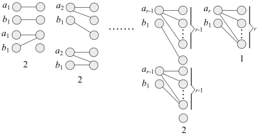
Proof. The first two terms in the formula count the number of unlabeled (2, r)-bipartite graphs in which one of the left vertices has zero degree and the degree of the other vertex varies between 0 and r. To count the remaining unlabeled (2, r)-bipartite graphs, we note that each left vertex can be connected up to r right vertices. Let ai denote the first left vertex2, where i indicates that ai is

connected to i right vertices, 1  i  r, and bj denote the second left vertex,

where j indicates that bj is connected to j right vertices, 1 j  r. Let (ai, bj

)-bipartite graph refer to any unlabeled )-bipartite graph in which the two left vertices are connected to i and j right vertices, respectively. Since reordering the left vertices in any (2, r)-bipartite graph results in an equivalent (2, r)-bipartite graph, any two (ai, bj)-bipartite graph and (aj, bi)-graph, 1  i, j  r are equivalent,

and they should therefore be counted only once. This counting constraint will be enforced by requiring that 1 _{ j  i  r. Now, there exist exactly two} distinct unlabeled (ai, b1)-bipartite graphs for each i, 1  i  r 1, and there

exists one (ar, b1)-bipartite graph (See Figure 2.2). Thus, there exist exactly

2(r 1) + 1 unlabeled (ai, bj)-bipartite graphs, 1 i  r and j = 1. Extending

the construction to the next case, it is not difficult to see that there exist 3(r

2_{This labeling of vertices is used to keep track of their degrees during the counting process}

3) + 2 + 1 (ai, bj)-bipartite graphs, 2  i  r and j = 2, and in general, there

exist (j + 1)(r 2j + 1) +Pj_k=1k = (j + 1)(r 3j/2 + 1) (ai, bj)-bipartite graphs,

1 j  r/2. Summing the last expression for 1  j  r/2 gives the third term in the formula in Eqn. 2.77. What remains unaccounted for are (ai, bj)-bipartite

graphs, r/2 + 1 j  i  r. These are counted using a similar argument, i.e., by creating new (ai, bj)-bipartite graphs by first fixing j to r/2 + 1, then to r/2 + 2,

and so on, while varying i between j and r in each case. It can be shown that the first case leads to r/2 unlabeled (2, r)-bipartite graphs, i.e., (ai, br/2+1)-bipartite

graphs, r/2 + 1 _{ i  r, the second case leads to r/2} 1 new unlabeled (2, r)-bipartite graphs, i.e., (ai, br/2+2)-bipartite graphs, r/2 + 2  i  r, and the last

case leads to just one new unlabeled (2, r)-bipartite graph, i.e., (ar, br)-bipartite

graph. Summing these up givesPr_j=r/2+1Pr_i=jr i + 1 = 1_{48 (r}3_{+ 6r}2_{+ 8r), i.e.,}

the last term in Eqn. 2.77 and the statement follows.

a

b

a

b

a

b

a

b

a

b

a

b

a

b

2

2

2

1

Figure 2.2: Construction of unlabeled (2, r)-bipartite graphs with exactly two left vertices, 1 i  r.

The odd r case is a direct corollary of the theorem. Corollary 1. For odd r,

|Bu(2, r)| = 1 + r + 1 16(r 3_{+ 7r}2 _{r 7) +} 1 48(r 3_{+ 9r}2_{+ 23r + 15). (2.78)}

Proof. To obtain Eqn. 2.78, it is sufficient to replace each occurrence of r/2 in the proof of theorem by (r 1)/2.

Remark 1. It is noted that the _|Bu(2, r)| formulas in Eqns. 2.77 and 2.78 can

be combined to give Eqn. 2.33. Moreover, |Bu(2, 2i 2)| coincides with the ith

hexagonal pyramidal number (see the integer sequence, A002412 in [34]), when i = 1, 2, 3, . . ..

Extension of the elementary proof of the formula _|Bu(n, r)| when n = 3 case

remains open. Moreover an exact computation _|Bu(n, r)| for n 4 also remains

open. In the next chapter, we will establish a two sided inequality for |Bu(n, r)|

Chapter 3

Bounds for Unlabeled Bipartite

Graphs

In this chapter, we provide a two sided inequality for _|Bu(n, r)| that then

estab-lishes an asympthotic formula for the same. More precisely, we prove

r+2n ₁

r

n!  |Bu(n, r)| 

2 r+2_rn 1

n! , n < r. (3.1)

We begin with our lower bound.

3.1

A Lower Bound for

_|B

(n, r)

|

From Eqns. 2.2 and 2.4 we know that

|Bu(n, r)| = ZSn⇥Sr(2, 2, . . . , 2), (3.2) = [ZSn(x1, x2,· · · , xn)⇥ ZSr(x1, x2,· · · , xr)](2, 2, . . . , 2). (3.3)

One of the terms in ZSn(x1, x2,· · · , xn) is

1 n!(x

n

1) and it is associated with the

identity permutation in Sn. Using this fact, we find

|Bu(n, r)| = ZSn⇥Sr(2, 2, . . . , 2), (3.4) = [ZSn(x1, x2,· · · , xn)⇥ ZSr(x1, x2,· · · , xr)](2, 2, . . . , 2), (3.5) = ✓ 1 n!(x n 1 + . . .) ◆ ⇥ ZSr(x1, x2,· · · , xr) (2, 2, . . . , 2), (3.6) = ✓ 1 n!x n 1 ◆ ⇥ ZSr(x1, x2, . . . , xr) (2, 2, . . . , 2) + . . . , (3.7) = 1 n! (_h xn₁ ⇥ 1 r! r! X t=1 r Y j=1 xqt,j j i (2, 2, ..., 2) ) + . . . , (3.8) = 1 n! ( h 1 r! r! X t=1 xn 1 K_Yr j=1 xqt,j j i (2, 2, ..., 2) ) + . . . , (3.9) = 1 n! ( h 1 r! r! X t=1 r Y j=1 xnqt,jgcd(1,j) lcm(1,j) i (2, 2, ..., 2) ) + . . . , (3.10) = 1 n! ( h 1 r! r! X t=1 r Y j=1 xnqt,j j i (2, 2, ..., 2) ) + . . . , (3.11) = 1 n! ( 1 r! r! X t=1 r Y j=1 2nqt,j ) + . . . , (3.12) = 1 n! ( 1 r! r! X t=1 r Y j=1 (2n)qt,j ) + . . . , (3.13) = 1 n! ( ZSr(2 n_{, 2}n_{, . . . , 2}n₎ ) + . . . . (3.14) This proves |Bu(n, r)| 1 n!ZSr(2 n_{, 2}n_{, . . . , 2}n_{). (3.15)} Proposition 1. ZSr(2 n_{, 2}n_{, . . . , 2}n_{) =} ✓ r + 2n ₁◆ (3.16)

Proof. Using Eqn. 2.5, we have rZSr(2 n_{, 2}n_{, . . . , 2}n_{) =} r X i=1 2nZSr i(2 n_{, 2}n_{, . . . , 2}n_{), (3.17)} and (r 1)ZSr 1(2 n_{, 2}n_{, . . . , 2}n_{) =} r 1 X i=1 2nZSr 1 i(2 n_{, 2}n_{, . . . , 2}n_{). (3.18)}

Subtracting the second equation from the first one gives

rZSr(2 n_{, 2}n_{, . . . , 2}n_{) (r 1)Z} Sr 1(2 n_{, 2}n_{, . . . , 2}n_{) = 2}n_Z Sr 1(2 n_{, 2}n_{, . . . , 2}n_), (3.19) rZSr(2 n_{, 2}n_{, . . . , 2}n_{) = (r + 2}n _1)Z Sr 1(2 n_{, 2}n_{, . . . , 2}n_), (3.20) ZSr(2 n_{, 2}n_{, . . . , 2}n_{) = (}r + 2n 1 r )ZSr 1(2 n_{, 2}n_{, . . . , 2}n_). (3.21)

Expanding the last equation inductively, we obtain

ZSr(2 n_{, 2}n_{, . . . , 2}n_{) = (}r + 2n 1 r )( r + 2n ₂ r 1 )ZSr 2(2 n_{, 2}n_{, . . . , 2}n_{), (3.22)} ZSr(2 n_{, 2}n_{, . . . , 2}n_{) = (}r + 2n 1 r )( r + 2n ₂ r 1 )( r + 2n ₃ r 2 )ZSr 3(2 n_{, 2}n_{, . . . , 2}n_), (3.23) ZSr(2 n_{, 2}n_{, . . . , 2}n_{) = (}r + 2n 1 r )( r + 2n ₂ r 1 )( r + 2n ₃ r 2 ) . . . ( 2n 1 )ZS0(). (3.24)

Noting that ZS0() = 1, and combining the product terms together, we obtain

ZSr(2 n_{, 2}n_{, . . . , 2}n_{) =} ✓ r + 2n ₁ r ◆ . (3.25)

Combining Proposition 1 with Eqn. 3.15 proves the lower bound. Theorem 4. |Bu(n, r)| r+2n ₁ r n! . (3.26)

3.2

An Upper Bound for

_|B

(n, r)

|

We first note that |Bu(1, r)| = r + 1 = r+2

1 ₁

r /1!  2

r+21 ₁

r /1!. Hence the

upper bound that is claimed in the beginning of this chapter holds for n = 1. Proving that it also holds for n 2 requires a more careful analysis of the terms in ZSn(x1, x2,· · · , xn)⇥ ZSr(x1, x2,· · · , xr). (3.27) We first express ZSn(x1, x2,· · · , xn) as ZSn(x1, x2, . . . , xn) = ZSn[1] + ZSn[2] + . . . + ZSn[n!], (3.28) where ZSn[1] = 1 n!x n 1, (3.29) ZSn[2] = 1 n!x n 2 1 x2. (3.30)

The first term is associated with the identity permutation and the second term is associated with any one of the permutations in which all but two of the elements in N = 1, 2,· · · , n are fixed to themselves. The remaining ZSn[i] =

1 n! Qn k=1x pi,k k , 3

i_{ n! terms represent all the other product terms in the cycle index polynomial} of Sn with no particular association with the permutations in Sn. Similarly, we

set ZSr(x1, x2, . . . , xr) = 1 r! Pr! t=1 Qr j=1x qt,j

j without identifying the actual product

terms with any particular permutation in Sr.

The following equations obviously hold as the sum of the lengths of all the cycles in any cycle disjoint representation of a permutation in Sn and Sr must be n and

n X k=1 kpi,k = n, 1 i  n!, (3.31) r X j=1 jqt,j = r, 1 t  r!. (3.32)

Now we can proceed with the computation of the upper bound for |Bu(n, r)|.

First, we note that

|Bu(n, r)| =ZSn⇥Sr(2, 2, 2, . . . , 2), (3.33) = [ZSn(x1, x2, . . . , xn)⇥ ZSr(x1, x2,· · · , xr)] (2, 2, . . . , 2), (3.34) = [(ZSn[1] + ZSn[2] + . . . + ZSn[n!])⇥ ZSr(x1, x2, . . . , xr)] (2, 2, . . . , 2), (3.35) = [ZSn[1]⇥ ZSr(x1, x2, . . . , xr)] (2, 2, . . . , 2) + [ZSn[2]⇥ ZSr(x1, x2, . . . , xr)] (2, 2, . . . , 2) + . . . + [ZSn[n!]⇥ ZSr(x1, x2, . . . , xr)] (2, 2, . . . , 2). (3.36)

The first term in Eqn. 3.36 is directly computed from Proposition 1. Thus, it suffices to upper bound each of the remaining terms in Eqn. 3.36 to upper bound _|Bu(n, r)|. This will be established by proving

[ZSn[2]⇥ ZSr(x1, x2, . . . , xr)] (2, 2, . . . , 2) [ZSn[i]⇥ ZSr(x1, x2, . . . , xr)] (2, 2, . . . , 2), 8i, 3  i  n!. We first need some preliminary facts.

Lemma 6. For all i, 1_{ i  n!,}

[ZSn[i]⇥ ZSr(x1, x2, . . . , xr)](2, . . . , 2) = 1 n!ZSr(2 Pn k=1pi,kgcd(k,1)_{, . . . , 2}Pnk=1pi,kgcd(k,r)_). (3.37)

Proof. [ZSn[i]⇥ ZSr(x1, . . . , xr)](2, . . . , 2) = " 1 n! n Y k=1 xpi,k k ⇥ 1 r! r! X t=1 r Y j=1 xqt,j j !# (2, . . . , 2), (3.38) = " 1 n!r! r! X t=1 n Y k=1 xpi,k k K_Yr j=1 xqt,j j # (2, . . . , 2), (3.39) = " 1 n!r! r! X t=1 r Y j=1 n Y k=1 xpi,kqt,jgcd(k,j) lcm(k,j) # (2, . . . , 2), (3.40) = 1 n!r! r! X t=1 r Y j=1 n Y k=1 2pi,kqt,jgcd(k,j)_{, (3.41)} = 1 n! " 1 r! r! X t=1 r Y j=1 (2Pnk=1pi,kgcd(k,j)₎qt,j # , (3.42) = 1 n!ZSr(2 Pn k=1pi,kgcd(k,1)_{, . . . , 2}Pnk=1pi,kgcd(k,r)_). (3.43) Corollary 2. [ZSn[2]⇥ ZSr(x1, x2, . . . , xr)](2, . . . , 2) = 1 n!ZSr(2 n 1_{, 2}n_{, 2}n 1_{, 2}n_{, . . .). (3.44)}

Proof. By definition, p2,1 = n 2, p2,2 = 1, p2,k = 0, 3  k  n. Substituting

these into the last equation in Lemma 6 proves the statement.

Lemma 7.

Pn

k=1pi,k  n 1,8i, 2  i  n!. (3.45)

Proof. Recall from Eqn. 3.31 that Pn_k=1kpi,k = n, 8i, 1  i  n!. Hence

Pn

k=1pi,k = n

Pn

k=1(k 1)pi,k, and so the maximum value of

Pn

k=1pi,k occurs

whenPn_k=1(k 1)pi,kis minimized. Furthermore, at least one of pi,k,8i, 2  i  n!

must be 1 for some k 2 since none of the permutations we consider is the identity. Thus,Pn (k 1)p 1 and the statement follows.

Lemma 8. If Pn_k=1pi,kgcd(k, ↵ + 1) = n, then Pn_k=1pi,kgcd(k, ↵)  n 1,

8i, 2  i  n! and for any integer ↵ 2.

Proof. If Pn_k=1pi,kgcd(k, ↵ + 1) = n as stated in the lemma, then we must have

gcd(k, ↵ + 1) = k where pi,k 1, 8i, 2  i  n!. Therefore k  ↵ + 1. Now if

k = ↵ + 1, then trivially gcd(k, ↵) < k. On the other hand if k < ↵ + 1, then ↵ + 1 must be a multiple of k. Therefore, ↵ can not be a multiple of k for any k 2. At this point we find that gcd(k, ↵) < k, _{8k, 2  k  n. Since as in the} previous lemma, none of the permutations we consider is the identity, at least one of pi,k,8i, 2  i  n! must be 1 for some k 2 and so we conclude that

Pn k=1pi,kgcd(k, ↵) n 1. Lemma 9. ZSr(2 n 1_{, 2}n_{, . . .) Z} Sr 1(2 n 1_{, 2}n_{, . . .), (3.46)} for 2_{ n.}

Proof. Using Eqn. 2.5, we get rZSr(2 n 1_{, 2}n_{, . . .) =} r_X1 odd i 2n 1ZSr i(2 n 1_{, 2}n_{, . . .) +} r_X2 even i 2nZSr i(2 n 1_{, 2}n_{, . . .),} (3.47)

where 1 = 1, 2= 0 if r is even and 1 = 0, 2 = 1 if r is odd.

Similarly, for r 1, (r 1)ZSr 1(2 n 1_{, 2}n_{, . . .) =} r 1X2 odd i 2n 1ZSr 1 i(2 n 1_{, 2}n_{, . . .)+} r 1X1 even i 2nZSr 1 i(2 n 1_{, 2}n_{, . . .).} (3.48)

Subtracting Eqn. 3.48 from Eqn. 3.47 gives rZSr(2 n 1_{, 2}n_{, . . .) (r 1)Z} Sr 1(2 n 1_{, 2}n_{, . . .)} = rX2 even i 2nZSr i(2 n 1_{, 2}n_{, . . .)} r 1X2 odd i 2n 1ZSr 1 i(2 n 1_{, 2}n_{. . .)} + r_X1 odd i 2n 1ZSr i(2 n 1_{, 2}n_{, . . .)} r 1_X1 even i 2nZSr 1 i(2 n 1_{, 2}n_{, . . .), (3.49)} rZSr(2 n 1_{, 2}n_{, . . .) (r 1)Z} Sr 1(2 n 1_{, 2}n_{, . . .)} = rX2 even i 2n 1_Z Sr i(2 n 1_{, 2}n_{, . . .) + 2}n 1_Z Sr 1(2 n 1_{, 2}n_{, . . .)} r 1X1 even i 2n 1_Z Sr 1 i(2 n 1_{, 2}n_{, . . .),} (3.50) rZSr(2 n 1_{, 2}n_{, . . .) = (r 1 + 2}n 1_)Z Sr 1(2 n 1_{, 2}n_{. . .)} + 2n 1 r_X2 even i ZSr i(2 n 1_{, 2}n_{, . . .)} r 1_X1 even i ZSr 1 i(2 n 1_{, 2}n_{, . . .)} ! . (3.51)

We now prove the lemma by induction on r. Basis r = 1. By Eqn. 2.5, ZS1(2 n 1_{) = 2}n 1_Z S0() = 2 n 1_{. So we have Z} S1(2 n 1_{) =} 2n 1 _Z S0() = 1 for 2 n.

Induction Step. Suppose that the lemma holds from 1 to r 1. That is, ZSr i ZSr i 1 0, 1 i  r 1. Now if r is even then the di↵erence of the two sums in Eqn. 3.51 becomes (ZSr 2 ZSr 3)+(ZSr 4 ZSr 5) . . .+(ZS2 ZS1)+ZS0, which is clearly 0 by the induction hypothesis. Therefore,

rZSr(2 n 1_{, 2}n_{, . . .) (r 1 + 2}n 1_)Z Sr 1(2 n 1_{, 2}n_{, . . .), (3.52)} ZSr(2 n 1_{, 2}n_{, . . .) Z} Sr 1(2 n 1_{, 2}n_{, . . .), n 2. (3.53)}

On the other hand, if r is odd then the di↵erence of the two sums in the same equation becomes (ZSr 2 ZSr 3) + (ZSr 4 ZSr 5) . . . + (ZS2 ZS1) + (ZS1 ZS0), which is again 0, and the statement follows in this case as well.

We now are ready to prove that [ZSn[2]⇥ ZSr(x1, x2, . . . , xr)](2,. . . ,2) [ZSn[i]⇥ ZSr(x1, x2, . . . , xr)](2,. . . ,2), (3.54) 8i, 2  i  n! and 8n, n < r. Theorem 5. [ZSn[2]⇥ ZSr(x1, x2, . . . , xr)](2, 2, . . . , 2) [ZSn[i]⇥ ZSr(x1, x2, . . . , xr)](2, 2, . . . , 2) (3.55) 8i, 2  i  n! and 8n, n < r.

Proof. Using Lemma 6 and Corollary 2 it suffices to show that ZSr(2

n 1_{, 2}n_{, . . .) Z} Sr(2

Pn

k=1pi,kgcd(k,1)_{, . . . , 2}Pnk=1pi,kgcd(k,r)_{). (3.56)} We prove the statement by induction on r.

Basis: (r = 1). By Eqn. 2.5, ZS1(2 n 1_{) = 2}n 1_Z S0() = 2 n 1_{. Similarly, by} Eqn. 2.5, ZS1(2 Pn k=1pi,kgcd(k,1)_{) = 2}Pnk=1pi,kgcd(k,1)_Z S0() = 2 Pn

k=1pi,k_{. Given that} Pn

k=1pi,k  n 1 by Lemma 7, we have 2 Pn

k=1pi,k _{ 2}n 1_{, and hence the statement} holds in this case.

Induction Step: First, by Eqn. 2.5,

ZSr(2 n 1_{, 2}n_{, . . .) =} 1 r 2 6 6 6 6 6 6 6 4 2n 1_Z Sr 1(2 n 1_{, 2}n_{, . . .)} +2n_Z Sr 2(2n 1, 2n, . . .) +2n 1_Z Sr 3(2 n 1_{, 2}n_{, . . .)} ... +2 ZS0() 3 7 7 7 7 7 7 7 5 , (3.57)

where = n if r is even and = n 1 if r is odd. Similarly,

ZSr(2 Pn k=1pi,kgcd(k,1)_{, . . . , 2}Pnk=1pi,kgcd(k,r)_{) =} 1 r 2 6 6 6 6 6 6 6 4 2Pnk=1pi,kgcd(k,1)_Z Sr 1(2 Pn k=1pi,kgcd(k,1)_{, . . .)} +2Pnk=1pi,kgcd(k,2)Z Sr 2(2 Pn k=1pi,kgcd(k,1), . . .) +2Pnk=1pi,kgcd(k,3)_Z Sr 3(2 Pn k=1pi,kgcd(k,1)_{, . . .)} ... +2Pnk=1pi,kgcd(k,r)Z S0() 3 7 7 7 7 7 7 7 5 . (3.58)

Subtracting Eqn. 3.58 from Eqn. 3.57, we have ZSr(2 n 1_{, 2}n_{, . . .) Z} Sr(2 Pn k=1pi,kgcd(k,1)_{, . . . , 2}Pnk=1pi,kgcd(k,r)₎ =1 r 2 6 6 6 6 6 6 6 4 2n 1_Z Sr 1(2 n 1_{, 2}n_{, . . .)} +2n_Z Sr 2(2n 1, 2n, . . .) +2n 1_Z Sr 3(2 n 1_{, 2}n_{, . . .)} ... +2 ZS0() 3 7 7 7 7 7 7 7 5 1 r 2 6 6 6 6 6 6 6 4 2Pnk=1pi,kgcd(k,1)_Z Sr 1(2 Pn k=1pi,kgcd(k,1)_{, 2}Pnk=1pi,kgcd(k,2)_{, . . .)} +2Pnk=1pi,kgcd(k,2)_Z Sr 2(2 Pn k=1pi,kgcd(k,1)_{, 2}Pnk=1pi,kgcd(k,2)_{, . . .)} +2Pnk=1pi,kgcd(k,3)_Z Sr 3(2 Pn k=1pi,kgcd(k,1)_{, 2}Pnk=1pi,kgcd(k,2)_{, . . .)} ... +2Pnk=1pi,kgcd(k,r)_Z S0() 3 7 7 7 7 7 7 7 5 . (3.59)

Thus, it suffices to show that the right hand side of the above equation is 0, or 2n 1_Z Sr 1(2n 1, 2n, . . .) 2 Pn k=1pi,kgcd(k,1)_Z Sr 1(2 Pn k=1pi,kgcd(k,1)_{, 2}Pnk=1pi,kgcd(k,2)_{, . . .)} +2n_Z Sr 2(2 n 1_{, 2}n_{, . . .) 2}Pn_k=1pi,kgcd(k,2)_Z Sr 2(2 Pn k=1pi,kgcd(k,1)_{, 2}Pnk=1pi,kgcd(k,2)_{, . . .} +2n 1_Z Sr 3(2n 1, 2n, . . .) 2 Pn k=1pi,kgcd(k,3)_Z Sr 3(2 Pn k=1pi,kgcd(k,1)_{, 2}Pnk=1pi,kgcd(k,2)_{, . . .)} ... +2 ZS0() 2 Pn k=1pi,kgcd(k,r)_Z S0() 0. (3.60) Now by induction hypothesis, Eqn. 3.56 holds for 1, 2,_{· · · , r 1. Thus, Eqn. 3.60} can be replaced by 2n 1_Z Sr 1(2 n 1_{, 2}n_{, . . .) 2}Pn_k=1pi,kgcd(k,1)_Z Sr 1(2 n 1_{, 2}n_{, . . .)} +2n_Z Sr 2(2 n 1_{, 2}n_{, . . .) 2}Pn k=1pi,kgcd(k,2)Z Sr 2(2 n 1_{, 2}n_{, . . .)} +2n 1_Z Sr 3(2 n 1_{, 2}n_{, . . .) 2}Pn_k=1pi,kgcd(k,3)_Z Sr 3(2 n 1_{, 2}n_{, . . .)} ... +2 ZS0() 2 Pn k=1pi,kgcd(k,r)Z S0() 0. (3.61)

Moreover, invoking Lemma 7 gives 2n 1ZSr 1(2 n 1_{, 2}n_{, . . .) 2}Pn_k=1pi,kgcd(k,1)_Z Sr 1(2 n 1_{, 2}n_{. . .)} 2n 1ZSr 1(2 n 1_{, 2}n_{, . . .) 2}n 1_Z Sr 1(2 n 1_{, 2}n_{, . . .) = 0.} (3.62)

Hence the di↵erence in the first line in Eqn. 3.61 0, and therefore it is sufficient to show that 2n_Z Sr 2(2 n 1_{, 2}n_{, . . .) 2}Pn_k=1pi,kgcd(k,2)_Z Sr 2(2 n 1_{, 2}n_{, . . .)} +2n 1_Z Sr 3(2 n 1_{, 2}n_{, . . .) 2}Pn_k=1pi,kgcd(k,3)Z Sr 3(2 n 1_{, 2}n_{, . . .)} ... +2 ZS0() 2 Pn k=1pi,kgcd(k,r)_Z S0() 0. (3.63)

To prove this inequality, we will combine four terms in pairs of consecutive lines for the remaining r 1 lines by considering two cases. If r is odd then = n 1 and no extra line remains in this pairing. Thus, for all even ↵, 2 ↵  r 1, it suffices to prove 2n_Z Sr ↵(2 n 1_{, 2}n_{, . . .) 2}Pn_k=1pi,kgcd(k,↵)_Z Sr ↵(2 n 1_{, 2}n_{. . .),} +2n 1_Z Sr ↵ 1(2 n 1_{, 2}n_{, . . .) 2}Pn_k=1pi,kgcd(k,↵+1)Z Sr ↵ 1(2 n 1_{, 2}n_{. . .) 0.} (3.64) or, 2n_Z Sr ↵(2 n 1_{, 2}n_{, . . .) 2}Pn_k=1pi,kk_Z Sr ↵(2 n 1_{, 2}n_{. . .)} +2n 1_Z Sr ↵ 1(2 n 1_{, 2}n_{, . . .) 2}Pn k=1pi,kgcd(k,↵+1)Z Sr ↵ 1(2 n 1_{, 2}n_{. . .) 0.} (3.65)

Now if Pn_k=1pi,kgcd(k, ↵ + 1) n 1, then

2nZSr ↵(2 n 1_{, 2}n_{, . . .) 2}Pn_k=1pi,kk_Z Sr ↵(2 n 1_{, 2}n_{, . . .)} + 2n 1ZSr ↵ 1(2 n 1_{, 2}n_{, . . .) 2}n 1_Z Sr ↵ 1(2 n 1_{, 2}n_{, . . .)} 2nZSr ↵(2 n 1_{, 2}n_{, . . .) 2}n_Z Sr ↵(2 n 1_{, 2}n_{, . . .) + 2}n 1_Z Sr ↵ 1(2 n 1_{, 2}n_{, . . .)} 2n 1_Z Sr ↵ 1(2 n 1_{, 2}n_{, . . .) = 0. (3.66)}

On the other hand, if Pn_k=1pi,kgcd(k, ↵ + 1) = n, then we prove Eqn. 3.64 by

noting that Pn_k=1pi,kgcd(k, ↵) n 1 by Lemma 8. Thus,

2nZSr ↵(2 n 1_{, 2}n_{, . . .) 2}n 1_Z Sr ↵(2 n 1_{, 2}n_{, . . .)} + 2n 1_Z Sr ↵ 1(2 n 1_{, 2}n_{, . . .) 2}n_Z Sr ↵ 1(2 n 1_{, 2}n_{, . . .)} = 2n 1ZSr ↵(2 n 1_{, 2}n_{, . . .) 2}n 1_Z Sr ↵ 1(2 n 1_{, 2}n_{, . . .)} 2n 1⇥ZSr ↵(2 n 1_{, 2}n_{, . . .) Z} Sr ↵ 1(2 n 1_{, 2}n_{, . . .)}⇤_{. (3.67)}

Now by Lemma 9, ZSr ↵(2

n 1_{, 2}n_{, . . .) Z}

Sr ↵ 1(2

n 1_{, 2}n_{, . . .) and the statement}

is proved for odd r, n < r. For even r, the last line in Eqn. 3.63 is left out in the pairing of consecutive lines and = n. In this case we have 2n_Z

S0() 2Pnk=1pi,kgcd(k,r)Z S0() 2 n_Z S0() 2 Pn k=1pi,kkZ S0() = 2 n_Z S0() 2 n_Z S0() = 0 and the statement follows.

Theorem 6. [ZSn[2]⇥ ZSr(x1, x2, . . . , xr)] (2, 2, . . . , 2) r+2n ₁ r n!(n! 1) (3.68) where 2_{ n < r.} Proof. By Corollary 2 [ZSn[2]⇥ ZSr(x1, x2, . . . , xr)] (2, 2, . . . , 2) = 1 n!ZSr(2 n 1_{, 2}n_{, . . .). (3.69)}

Thus, to prove the theorem, it is sufficient to show 1 n!ZSr(2 n 1_{, 2}n_{, 2}n 1_{, 2}n_{, . . .)} r+2n ₁ r n!(n! 1) (3.70) where 2_{ n < r.}

Now, using Eqn. 2.5, we get rZSr(2 n 1_{, 2}n_{, . . .) =} r_X1 odd i 2n 1ZSr i(2 n 1_{, 2}n_{, . . .) +} r_X2 even i 2nZSr i(2 n 1_{, 2}n_{, . . .)} (3.71)

where 1 = 1, 2 = 0 if r is even and 1 = 0, 2 = 1 if r is odd. Similarly, for

r 2, (r 2)ZSr 2(2 n 1_{, 2}n_{, . . .) =} r 2X1 odd i 2n 1_Z Sr 2 i(2 n 1_{, 2}n_{, . . .) +} r 2X2 even i 2n_Z Sr 2 i(2 n 1_{, 2}n_{, . . .).} (3.72)

Subtracting Eqn. 3.72 from Eqn. 3.71 gives rZSr(2 n 1_{, 2}n_{, . . .) (r 2)Z} Sr 2(2 n 1_{, 2}n_{, . . .)} = 2n 1ZSr 1(2 n 1_{, 2}n_{, . . .) + 2}n_Z Sr 2(2 n 1_{, 2}n_{, . . .), (3.73)} rZSr(2 n 1_{, 2}n_{, . . .) = 2}n 1_Z Sr 1(2 n 1_{, 2}n_{, . . .) + (r 2 + 2}n_)Z Sr 2(2 n 1_{, 2}n_{, . . .),} (3.74) ZSr(2 n 1_{, 2}n_{, . . .) =} 1 r ⇥ 2n 1ZSr 1(2 n 1_{, 2}n_{, . . .) + (r 2 + 2}n_)Z Sr 2(2 n 1_{, 2}n_{, . . .)}⇤_. (3.75) We will use induction on r and the recurrence given in Eqn. 3.75 to prove this inequality.

Basis

Case 1: r = 3. Recall that ZSn[2] = 1 n!x n 2 1 x2, (3.76) ZS3(x1, x2, x3) = 1 3!(x 3 1+ 3x1x2+ 2x3). (3.77) Thus, [ZSn[2]⇥ ZS3(x1, x2, x3)] (2, 2, . . . , 2) =  1 n!(x n 2 1 x2)⇥ 1 3!(x 3 1+ 3x1x2+ 2x3) (2, 2, . . . , 2), (3.78) = 1 3!n! h (xn 2₁ x2) K x3₁+ (xn 2₁ x2) K (3x1x2) + (xn 21 x2) K 2x3 i (2, 2, . . . , 2), (3.79) = 1 3!n! h x3(n 2)₁ x3₂+ 3xn 2₁ x2xn 22 x22+ 2xn 23 x6 i (2, 2, . . . , 2), (3.80) = 1 3!n! ⇥ 23n 3+ 3_{⇥ 2}2n 1+ 2n⇤_ r+2n ₁ r n!(n! 1). (3.81) for n = 2 and r = 3.

Case 2: r = 4. In this case we have [ZSn[2]⇥ ZS4(x1, x2, x3, x4)] (2, . . . , 2) =  1 n!(x n 2 1 x2)⇥ 1 4!(x 4 1+ 6x21x2+ 3x22+ 8x1x3+ 6x4) (2, . . . , 2), (3.82) = 1 4!n!  (xn 2₁ x2) K x4₁+ (xn 2₁ x2) K (6x2₁x2) + (xn 21 x2) K 3x2₂ + (xn 2₁ x2) K (8x1x3) + (xn 21 x2) K 6x4 (2, . . . , 2), (3.83) = 1 4!n! h x4(n 2)₁ x4₂+ 6x2(n 2)₁ xn 2₂ x2₂x2₂+ 3x₁2(n 2)x4₂+ 8xn 2₁ xn 2₃ x2x6+ 6xn 24 x24 i (2, . . . , 2), (3.84) = 1 4!n! ⇥ 24n 4+ 6⇥ 23n 2_{+ 3⇥ 2}2n_{+ 8⇥ 2}2n 2_{+ 6⇥ 2}n⇤_{, (3.85)} = 1 4!n! ⇥ 24n 4_{+ 6⇥ 2}3n 2_{+ 5⇥ 2}2n_{+ 6⇥ 2}n⇤_{. (3.86)}

Now, given that r = 4, the only possible values of n are 2 and 3. If n = 2 then: [ZSn[2]⇥ ZS4(x1, x2, x3, x4)] (2, 2, . . . , 2) = 1 4!n! ⇥ 24n 4+ 6⇥ 23n 2_{+ 5⇥ 2}2n_{+ 6⇥ 2}n⇤_, (3.87) = 1 4!2! ⇥ 24+ 6⇥ 24_{+ 5⇥ 2}4_{+ 6⇥ 2}2⇤_, (3.88) = 16 + 96 + 80 + 24 4!2! = 4.5, (3.89)  r+2n ₁ r n!(n! 1) = 7 4 2!(2! 1) = 35 2 = 17.5. (3.90)

On the other hand, if n = 3 then: [ZSn[2]⇥ ZS4(x1, x2, x3, x4)] (2, . . . , 2) = 1 4!n! ⇥ 24n 4+ 6_{⇥ 2}3n 2+ 5_{⇥ 2}2n+ 6_{⇥ 2}n⇤, (3.91) = 1 4!3! ⇥ 28+ 6⇥ 27_{+ 5⇥ 2}6_{+ 6⇥ 2}3⇤_, (3.92)

[ZSn[2]⇥ ZS4(x1, x2, x3, x4)] (2, . . . , 2) = 256 + 768 + 320 + 48 4!3! = 29 3, (3.93)  r+2n ₁ r n!(n! 1) = 11 4 3!(3! 1) = 330 30 = 11. (3.94)

Induction Step: Suppose that Eqn. 3.70 holds for all values from 3 to r 1. Using the recurrence given in Eqn. 3.75 and the induction hypothesis for r 1 and r 2 we get 1 n!ZSr(2 n 1_{, 2}n_{, . . .) =} 1 n!r ⇥ 2n 1ZSr 1(2 n 1_{, 2}n_{, . . .) + (r 2 + 2}n_)Z Sr 2(2 n 1_{, 2}n_{, . . .)}⇤_, (3.95) = 2 n 1 n!r ZSr 1(2 n 1_{, 2}n_{, . . .) +} r 2 + 2n n!r ZSr 2(2 n 1_{, 2}n_{, . . .),} (3.96)  2 n 1 r r+2n ₂ r 1 n!(n! 1) + r 2 + 2n r r+2n ₃ r 2 n!(n! 1), (3.97)  2 n 1 n!(n! 1)r (r + 2n _2)! (r 1)!(2n _1)!+ r 2 + 2n n!(n! 1)r (r + 2n _3)! (r 2)!(2n _1)!, (3.98)  2 n 1 n!(n! 1)r (r + 2n _2)! (r 1)!(2n _1)!+ (r 1)(r + 2n _2)! n!(n! 1)r!(2n _1)!, (3.99)  (r + 2 n _{2)!(r + 2}n 1 ₁₎ n!(n! 1)r!(2n _1)!  (r + 2n _{2)!(r + 2}n ₁₎ n!(n! 1)r!(2n _1)! , (3.100)  (r + 2 n _1)! n!(n! 1)r!(2n _1)! = 1 n!(n! 1) ✓ r + 2n ₁ r ◆ , (3.101)  _n!(n!1 ₁₎ ✓ r + 2n ₁ r ◆ , (3.102)

and this completes the proof.

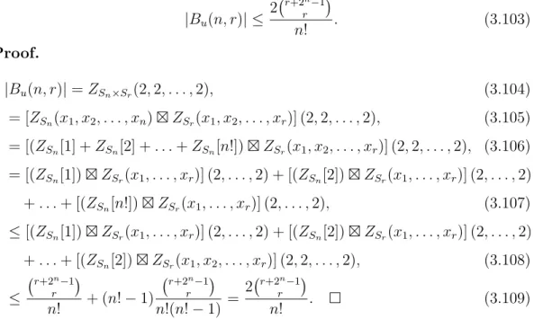
Theorem 7. |Bu(n, r)|  2 r+2_rn 1 n! . (3.103) Proof. |Bu(n, r)| = ZSn⇥Sr(2, 2, . . . , 2), (3.104) = [ZSn(x1, x2, . . . , xn)⇥ ZSr(x1, x2, . . . , xr)] (2, 2, . . . , 2), (3.105) = [(ZSn[1] + ZSn[2] + . . . + ZSn[n!])⇥ ZSr(x1, x2, . . . , xr)] (2, 2, . . . , 2), (3.106) = [(ZSn[1])⇥ ZSr(x1, . . . , xr)] (2, . . . , 2) + [(ZSn[2])⇥ ZSr(x1, . . . , xr)] (2, . . . , 2) + . . . + [(ZSn[n!])⇥ ZSr(x1, . . . , xr)] (2, . . . , 2), (3.107)  [(ZSn[1])⇥ ZSr(x1, . . . , xr)] (2, . . . , 2) + [(ZSn[2])⇥ ZSr(x1, . . . , xr)] (2, . . . , 2) + . . . + [(ZSn[2])⇥ ZSr(x1, x2, . . . , xr)] (2, 2, . . . , 2), (3.108)  r+2n ₁ r n! + (n! 1) r+2n ₁ r n!(n! 1) = 2 r+2_rn 1 n! . (3.109)

Table 3.1 lists ln_|Bu(n, r)| along with the natural logarithms of lower and upper

bounds for 1 n < r  15.

Remark 2. It should be mentioned that, if r < n, using the relation|Bu(n, r)| =

|Bu(r, n)| gives

|Bu(n, r)|  2

n+2r ₁

n

r! . (3.110)

Likewise, if r < n, Theorem 4 and_|Bu(n, r)| = |Bu(r, n)| together imply

|Bu(n, r)|

n+2r ₁

n

r! . (3.111)

Furthermore, if r = n, using the cycle index representation of bi-colored graphs provided in Section 3 in [23] and Theorem 4 gives

|Bu(n, n)|

n+2n ₁

n

2n! . (3.112)

The Z0_{term in the cycle index representation of bi-colored graphs in [23] prevents}

us from deriving an upper bound for _|Bu(n, n)| that is a constant multiple of

the lower bound in this case. On the other hand, an obvious upper bound for |B (n, n)_{| can be derived by setting r = n + 1 in the inequality in Theorem 7.}

n r 2 3 4 5 6 7 8 9 10 11 12 13 14 15 1 1.09861 1.09861 1.79176 1.38629 1.38629 2.07944 1.60944 1.60944 2.30259 1.79176 1.79176 2.48491 1.94591 1.94591 2.63906 2.07944 2.07944 2.77259 2.19722 2.19722 2.89037 2.30259 2.30259 2.99573 2.3979 2.3979 3.09104 2.48491 2.48491 3.17805 2.56495 2.56495 3.2581 2.63906 2.63906 3.3322 2.70805 2.70805 3.4012 2.77259 2.77259 3.46574 2 2.30259 2.56495 2.99573 2.83321 3.09104 3.55535 3.3322 3.52636 4.02535 3.73767 3.91202 4.43082 4.09434 4.2485 4.78749 4.40672 4.55388 5.10595 4.70048 4.82831 5.39363 4.96284 5.0814 5.65599 5.20401 5.31321 5.89715 5.42495 5.52943 6.1203 5.63479 5.7301 6.32794 5.82895 5.91889 6.52209 6.01127 6.09582 6.70441 3 4.00733 4.46591 4.70048 4.8828 5.24702 5.57595 5.65599 5.95584 6.34914 6.34914 6.59851 7.04229 6.97728 7.18841 7.67089 7.55276 7.73368 8.24617 8.08364 8.24012 8.77678 8.57622 8.71276 9.26936 9.03575 9.1562 9.7289 9.46653 9.57345 10.1597 9.872 9.96754 10.5651 10.255 10.3409 10.9481 4 6.4708 6.9594 7.16395 7.72356 8.08641 8.41671 8.86869 9.14238 9.56184 9.92471 10.1349 10.6179 10.9056 11.0692 11.5987 11.8219 11.9512 12.515 12.6821 12.7855 13.3752 13.493 13.5767 14.1861 14.2603 14.3287 14.9534 14.9885 15.045 15.6816 15.6816 15.7287 16.3748 5 9.87164 10.2603 10.5648 11.5633 11.826 12.2565 13.1474 13.3276 13.8406 14.6391 14.7645 15.3322 16.0501 16.1388 16.7432 17.3899 17.4535 18.083 18.6662 18.7124 19.3593 19.8854 19.9195 20.5785 21.053 21.0784 21.7461 22.1736 22.1927 22.8667 6 14.3253 14.5771 15.0185 16.5086 16.6637 17.2017 18.588 18.6849 19.2811 20.5759 20.6372 21.269 22.482 22.5215 23.1752 24.3146 24.3403 25.0078 26.0804 26.0974 26.7736 27.7852 27.7965 28.4783 29.4338 29.4415 30.127 7 19.9011 20.0463 20.5942 22.6165 22.6996 23.3097 25.2339 25.282 25.927 27.7633 27.7915 28.4564 30.2128 30.2295 30.906 32.5895 32.5995 33.2827 34.8992 34.9053 35.5924 37.147 37.1507 37.8401 8 26.6393 26.7201 27.3324 29.9164 29.9604 30.6096 33.102 33.1261 33.7952 36.2043 36.2177 36.8975 39.2304 39.2378 39.9235 42.186 42.1902 42.8792 45.0764 45.0788 45.7696 9 34.5644 34.6096 35.2575 38.4241 38.4479 39.1173 42.1988 42.2114 42.892 45.8953 45.902 46.5885 49.5197 49.5233 50.2128 53.0769 53.0789 53.7701 10 43.693 43.7187 44.3861 48.1502 48.1635 48.8434 52.5284 52.5353 53.2216 56.8335 56.837 57.5266 61.0705 61.0723 61.7636 11 54.0381 54.0528 54.7312 59.1036 59.1111 59.7967 64.0955 64.0993 64.7886 69.0189 69.0208 69.712 12 65.6106 65.6191 66.3038 71.2925 71.2968 71.9856 76.9056 76.9078 77.5988 13 78.4205 78.4254 79.1137 84.7251 84.7275 85.4182 14 92.4768 92.4797 93.17

Table 3.1: Exact values of ln|Bu(n, r)|, 1  n < r  15, and natural logarithms

of lower and upper bounds.

We conclude this chapter by stating that the constant factor of 2 in the upper bound can potentially be reduced further. However this will require a further reduction in Inequality 3.68, but reducing 1/(n! 1) in this inequality further seems difficult. Another alternative for reducing the constant in the upper bound would be to bound the remaining terms by a di↵erent technique, and this remains to be settled with further research.

Chapter 4

Labeled Bipartite Graphs

In this chapter, we will extend the bounds given in previous chapter to labeled bi-partite graphs. In particular, we introduce left(right)-set-labeled and set-labeled bipartite graphs and provide asymptotic bounds for their sizes.

4.1

Preliminary Facts

We begin with some definitions. An (n, r)-bipartite graph is called left(right)-set-labeled if its left(right) vertices are distinguishable up to subsets of all left(right) vertices. An (n, r)-bipartite graph is called set-labeled if left vertices are distin-guishable up to subsets of all left vertices and right vertices are distindistin-guishable up to subsets of all right vertices.

4.2

Left-Set-Labeled Bipartite Graphs

In this section, we start with counting four families of left-set-labeled bipartite graphs and then provide a lower and an upper bound on the number of left-set-labeled bipartite graphs. Right-set-left-set-labeled bipartite graphs are counted similarly and their counting is omitted.

Let Bx(n, r) be the set of all (n, r)-left-set-labeled bipartite graphs. Let Bx(n, r, i)

be the set of (n, r)-left-set-labeled bipartite graphs in each of which the degrees of exactly i left vertices are greater than 0. Let Bx(i, r) be the set of all (i,

r)-unlabeled bipartite graphs in each of which the degrees of all left vertices are greater than 0. It follows that

|Bx(n, r, i)| = ✓ n i ◆ |Bx(i, r)|. (4.1) |Bx(n, r)| = 1 + n X i=1 |Bx(n, r, i)|. (4.2) |Bx(n, r)| = 1 + n X i=1 ✓ n i ◆ |Bx(i, r)|. (4.3)

4.2.1

Counting Left-Set-Labeled Bipartite Graphs

Recall that Bu(n, r) denote the set of all unlabeled (n, r)-bipartite graphs. In

chapter 2, it was stated that_|Bu(1, r)| = r + 1. Dropping the empty graph yields

|Bx(1, r)| = r, and hence |Bx(1, r)| = r + 1. To compute |Bx(n, r)|, n 2 we

note the following identities.

|Bu(n, r)| = 1 + n X i=1 |Bx(i, r)|, (4.4) |Bu(n 1, r)| = 1 + n 1 X i=1 |Bx(i, r)|. (4.5)