The application of stochastic processes in exchange rate forecasting: benchmark test for the EUR/USD and the USD/TRY

(1)

Giray GOZGOR, PhD

Dogus University

Istanbul, Turkey

E-mail: ggozgor@dogus.edu.tr

THE APPLICATION OF STOCHASTIC PROCESSES IN

EXCHANGE RATE FORECASTING: BENCHMARK TEST FOR

THE EUR/USD AND THE USD/TRY

Abstract. This paper investigates the short-time exchange rate predictability in a developed and in an emerging market, and for this purpose we consider the Euro/United States Dollar (EUR/USD) and the United States Dollar/Turkish Lira (USD/TRY) exchange rates. We apply the benchmark test and compare the results of daily out-of-sample forecasting by Brownian Motion (BM), Geometric Brownian Motion (GBM), Ornstein-Uhlenbeck Mean-reversion (OUM), Jump Diffusion (JD) stochastic processes, Vector Autoregressive (VAR), Autoregressive Integrated Moving Average (ARIMA) models and Uncovered Interest Rate Parity (UCIP) against the Random Walk (RW). We conclude that none of these models or stochastic processes displays superiority over the RW model in forecasting the USD/TRY exchange rate. However, GBM, BM and OUM processes beat the RW model in forecasting the EUR/USD exchange rate. Furthermore, we show that these findings are robust and not time-specific. When we separately examine the pre-crisis and the post-crisis periods, results remain unchanged.

Key Words: Exchange Rate Predictability; Brownian motion; Mean-reversion; Jump Diffusion; GARCH Models; Probability Distributions.

JEL Classification: C53, F31, F47 1. Introduction

Since collapse of the Bretton Woods System in early 1970s, studies about forecasting performance of models for exchange rate determination have been taking an increasing share in international economics literature. Seminal papers of Meese and Rogoff (1983a, 1983b) indicated that any structural model (using fundamental macroeconomic variables, such as gross domestic product, money supply, interest rates and inflation rates) and time series techniques have not outperformed the simple random walk model in the out-of-sample forecasting. Similar diverse empirical findings make researchers think in a consensus that

(2)

Giray Gozgor

________________________________________________________________ exchange rates may follow a martingale difference sequence, and the exchange rate predictability cannot be possible with current available information or variables.1 This is known as the ‘exchange rate disconnect puzzle’ or the ‘Meese-Rogoff puzzle’ in the literature. Mark (1995) firstly pointed out that structural models might beat the random walk model in both out-of-sample and in-sample forecasting for the long-run. However, his general evidence on exchange rate predictability was only valid in the two year forecasting period or in the longer term. Cheung et al. (2005) clearly showed that none of structural model, specification or their combinations was able to show a success in the exchange rate forecasting. Actually, some models showed a ‘better performance’ than the random walk at the certain horizon and for the certain selection criteria. It might also be possible that one model would be “well-performed” for an exchange rate. However, their robust empirical evidences suggested that the Meese-Rogoff puzzle has still not unraveled. In that time, the literature about the exchange rate predictability was almost accepted validation of the Meese-Rogoff puzzle. However, a key suggestion for solution of the Meese-Rogoff puzzle was introduced by Engel and West (2005). In the rational expectations present-value model, they demonstrated that exchange rates follow near-random walk process and the factor for discounting future fundamentals is also near one. In their asset-pricing model for exchange rates, value of exchange rates can be linked to the fundamentals, if one uses forward-looking variables of the monetary policy or the reaction function of central banks. Engel et al. (2008) then used the panel data techniques in the forward-looking variables of monetary policy tools, and showed that structural models were able to beat the simple random walk. Rogoff (2008) commented about the empirical findings of Engel et al. (2008) such that: “Right now, things still look pretty good if we can call the glass 10 percent full”. Recent and ongoing literature still tries to fill the “glass”.2

The mentioned improvements in the above have eventuated in the middle-term or the long-term exchange rate forecasting literature. However, there is nearly no evidence about the short-term exchange rate predictability.3 So, the short-term exchange predictability has not adequately taken into consideration and this issue can be called as the ‘short-run exchange rate disconnect puzzle’. This paper investigates the short-run exchange rate predictability, and it suggests that a novel solution for the short-run exchange rate disconnect puzzle. In this study we use Brownian Motion (BM), Geometric Brownian Motion (GBM), Ornstein-Uhlenbeck Mean-reversion (OUM) and Jump Diffusion (JD) stochastic processes

1_{The terms of ‘random-walk’ and ‘martingale’ are interchangeably used in the literature.} However, strictly speaking, the series are independent and identically distributed (iid) for ‘random-walk’, while there is a martingale difference sequence (mds) for a ‘martingale’. 2

See Rossi (2013) for a brief review of the recent literature.

3_{For example, Cheong et al. (2012) recently showed that the daily exchange rates may} follow a martingale difference sequence, so it can be said that ‘short-run exchange rate disconnect puzzle’ still remains.

(3)

The Application of Stochastic Processes in Exchange Rate Forecasting: Benchmark test for the EUR/USD and the USD/TRY

___________________________________________________________

and performed their out-of-sample forecasting results against random walk at daily frequency sample. We also include Vector Autoregression (VAR), Autoregressive Integrated Moving Average (ARIMA) and Uncovered Interest Rate Parity models in the paper. In fact, our interest for related stochastic processes basically comes from two facts. First, fundamentals, such as inflation rate, money supply or gross domestic products are not yet available at the daily frequency. So, related stochastic processes could provide an alternative and a further methodology for solution of the short-run exchange rate disconnect puzzle. Second, despite some kind of stochastic process are commonly used in the forecasting of interest rate, oil and agricultural commodity prices, and their futures markets prices4, they have not adequately used for the nominal exchange rate forecasting.5 Thus, main contribution of this paper is to define a standard methodology using mentioned stochastic processes in order to solve the short-run exchange rate disconnect puzzle. So, first hypothesis in this study is that at least one of the stochastic processes will significantly be able to beat the naive random walk model. As we have already mentioned, this study focuses on both developed (the EUR/USD) and emerging (the USD/TRY) exchange rate markets. So, another hypothesis is tested that different stochastic processes may display superiority over the random walk model, when we separately investigate the forecasting performances of the developed and the emerging exchange rate market. Furthermore, we separately examine the pre-crisis and the post-crisis periods, so another hypothesis is that different stochastic processes may beat the random walk model in the pre-crisis, the crisis and the post-crisis periods.

The remainder of the paper is organized as follows. Section 2 explains the data and the methodology, section 3 discusses the empirical results, section 4 checks robustness of the empirical results, and section 5 is the concluding remarks.

2. Data and Methodology

This study based on 3182 daily spot exchange rate data from 4/1/1999 to 31/08/2011 for the EUR/USD. We obtain the data from database of the Federal Reserve Board (FED). We also use 2645 daily exchange rate data from 21/2/2001 to 31/08/2011 for the USD/TRY. The main reason to select this time period for the USD/TRY comes from the fact that the floating exchange rate regimes have taken effect in the Turkish Exchange Markets over the related period. The USD/TRY

4_{For an example, see Schwartz (1997).}

5_{Wang and Zong (2009) also used the Markov stochastic process for the nominal exchange} rate forecasting. Actually, we suggest the systematic methodology in asset price forecasting, such as that proposed by Brigo et al. (2009a, 2009b). We think that their papers are described to use the stochastic process for the exchange rate forecasting. In this study we follow their suggestions to compute daily exchange rate forecasting within the systematic methodology.

(4)

Giray Gozgor

________________________________________________________________ data are calculated as average of the “ask” and the “bid” rates for closed time in a day. We obtain the data from database of the Central Bank of Turkey (CBRT). Furthermore, if the domestic market is closed, but foreign market is opened in a day, we use the data of previous day for domestic market and vice versa. Our first exchange rate forecast starts from June 1, 2007, and they are kept going to the last observation. We follow the recursive scheme out-of-sample forecasting technique for both exchange rates. Selection of June 1, 2007 as a starting date of the out-of-sample forecasting is basically important for one reason. This starting date allows concurrently investigating the pre-crisis, the crisis and the post-crisis periods. The global crisis started in the middle 2007; however, it fully impacted the global exchange rate markets from July 2008 to February 2009 (Fratzscher 2009).In this study we therefore define the ‘crisis period’ from July 1, 2008 to February 1, 2009.

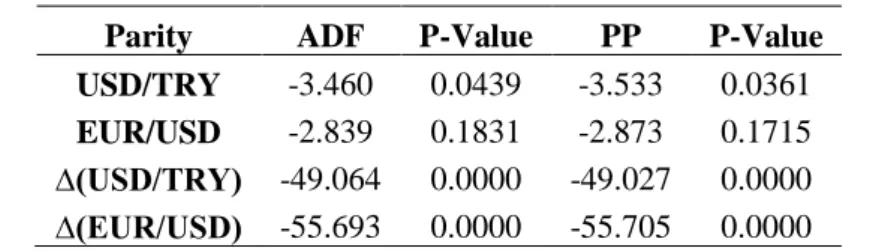
We firstly test the basic assumption of stationary exchange rates, and apply the Augmented Dickey Fuller (ADF) and the Phillips-Perron (PP) unit root tests into the natural logarithm of the EUR/USD and the USD/TRY. We report the results in Table 1 as follows:

Table 1. Results of the Unit Root Tests for the EUR/USD and the USD/TRY

Parity ADF P-Value PP P-Value

USD/TRY -3.460 0.0439 -3.533 0.0361 EUR/USD -2.839 0.1831 -2.873 0.1715 ∆(USD/TRY) -49.064 0.0000 -49.027 0.0000 ∆(EUR/USD) -55.693 0.0000 -55.705 0.0000

Notes: The table shows the results of the Dickey-Fuller and the Phillips-Perron unit root

tests, and results both include the constant and the trend terms. In these unit root tests the null hypothesis of that series have unit root. The optimal number of lag is selected by the Schwarz Criteria (SC) and the maximum number for lag is 28. We use the bandwidth selection method of Newey-West and the Barlett Kernel for the Phillips-Perron test. The critical values at the 5% and at the 1% significance levels are 3.411 and 3.961, respectively. The p-values are the one-sided MacKinnon probability values.

All results in Table 1 show that exchange rates in logarithmic form are stationary. We state the data and the basic properties of the exchange rates; thus we can explain the methodology for the exchange rate forecasting. We use eight methods for exchange rate forecasting and define them as follows:

(1) Random Walk: Following the seminal paper of Meese and Rogoff (1983a), we use the Random walk without drift (RWw) as a benchmark model, and define it as follows:

X

n



X

n1





n (1) In this equation,

X

_n is the value of exchange rate at current day,

X

_n_₁ is the exchange rate at previous day, and



_n is the error term and it has zero mean and iid.

(5)

___________________________________________________________

(2) Uncovered Interest Rate Parity (UCIP): In this study we use two interest rates for calculating the UCIP. First is the target or the policy rate of the central banks, and second is the yield of the benchmark government bonds. We use the marginal lending facility rate of the European Central Bank (ECB) and yield of the public debt securities for the EUR; the FED funds effective target rate and the yield of the four weeks treasury bills for the USD; and the overnight lending rate of the CBRT and the yield of the benchmark government debt securities for the TRY. We obtain related data from databases of the CBRT, the FED and the Deutsche Bundesbank, and calculate the UCIP as follows:

* 1 1 t t o t F i S i    (2) In this equation, i_tis the domestic interest rate, *

t

i is the foreign interest rate, So is the spot exchange rate, and F_tis the forward exchange rate.

(3) ARIMA (p,d,q): We use the ARIMA (p,d,q) model in the recursive scheme forecasting, and define it as follows:

  St 1 St1 2 St2 ... pSt p    t 1 t1 2 t2 ...  q t q (3) In this equation,



S

_tis the first difference of the natural logarithm of the exchange rate at time t,



is the autocorrelation coefficient of AR (p) and



_t is the coefficient of MA (q) models, respectively. We select the best fitting ARIMA (p,d,q) model by the Akaike Information Criteria (AIC) and the SC for the USD/TRY and the EUR/USD.

(4) VAR (p): We also use the VAR (p) model in the recursive scheme forecasting, and write it as follows:

yt 1yt1 ... pytp xtt (4)

In this equation,X_tis an (nx1) vector of endogenous variables (included as the difference between domestic interest rate and foreign interest rate) as well as the exchange rate, and



_tis a vector of white noise error terms. We select the best fitting lag structure for the VAR (p) model by the AIC and the SC for the USD/TRY and the EUR/USD. Thus, the basic models for exchange rates forecasting could easily be written as follows:

(6)

Giray Gozgor ________________________________________________________________ 1 1

(R

R

)

m m it it it j it it j it j j

USDTRY

c



USDTRY

_



try

usd

_

u

 

 









 

(5) 1 1

(R

Re

)

m m jt jt it j jt it j jt j j

EURUSD

c



EURUSD

_



usd

ur

_

u

 

 









 

(6)

(5) Brownian Motion: Firstly, we set some standard assumptions for stochastic process: (1) number of iteration or simulation is 1000 and the simple average of the simulation results are accepted as the ‘forecast’ for related day (2) number of the step or the path is 1000 for every stochastic process (3) we don’t use a random seed, and the forecasting period is only one day (4) we employ the out-of-sample recursive scheme methodology in the exchange rate forecasting. At this point, we define a simple Brownian motion process as follows:

dY dtdX (7) In this equation,



is the drift rate and  is the standard deviation or the volatility term.

(6) Geometric Brownian Motion: We define a simple Geometric Brownian motion process as follows:

2 1 (1 ) 2 dS 



S



S dt



SdZ (8)

In this equation,Spresents the value of the exchange rate.

(7) Uhlenbeck Mean-reversion: We define a simple Ornstein-Uhlenbeck Mean-reversion process as follows:

dr

t



 

(



r dt

t

)





dZ

t (9) In this equation,(



r_t)is the diversion from the long-term value of exchange rate,is the mean-reversion rate and



is the volatility term.

(8) Jump Diffusion Process: We define a simple Jump Diffusion Process as follows: dX t( )a X t dt( , ) b X t dZ t( , ) ( )h J X t dN( , , ) ( )



(10) 0;1 probability, ( ) 1;1 probability dt and dN dt         _   

(7)

___________________________________________________________

In this equation, h J X t( , , )is the jump size,

dN

( )



is the jump rate. The part of

a X t dt b X t dZ t

( , )



( , )

( )

is a simple Ito stochastic process with the drift parameter ( a ) and the volatility term (b).

Moreover, we define the mandatory parameters as follows. Drift rate is the return of last 20 days, long-term value is the value of exchange rate which is defined by the Consumer Price Index (CPI) based Purchasing Power Parity (PPP) condition, mean-reversion rate is the absolute return of last 200 days, jump rate is the simple average of extreme values6 in last 4 days, jump size is the number of extreme value days in last 4 days.7 The stochastic processes used in this study are basically generated by the Java and the SQL based algorithms. On the other hand, A stochastic process has three parts: These are the ‘mean part’ based on past returns, the ‘variance part’ based on volatility values, and the ‘random part’ based on probability distributions. At this point, we also need two parameters to compute the stochastic processes for the exchange rate forecasting; namely, the random terms (or the probability distributions) and the volatility terms.

Probability Distributions:

The probability distributions mentioned below will constitute the random part of the stochastic processes in exchange rate forecasting. We firstly determine the probability distribution of return of the last 252 days, according to the goodness of fit tests of Anderson and Darling (AD) and Kolmogorov and Smirnoff (KS). We select the probability distributions from distributions that are able to generate not only negative and positive changes in exchange rate returns, but also able to generate random negative numbers and extreme values if necessary. At this point, the methodology of random numbers generation strictly sticks to the last parameter values in the probability distributions. Moreover, obtained random numbers are constant for each day due to the performances of the stochastic processes will be compared. Thus we need same random numbers for all stochastic processes in a day. Hence the changes in best fitting probability distributions and/or parameters for each day are reflected to the all stochastic processes as such. We then use the probability distribution and related parameters to generate the random numbers in a rolling window scheme. The most common probability distributions that we used in this study can be written as follows:

Normal distribution, if real-valued random X variable XЄ (-∞,∞), µ is the mean and σ2

is the variance, the equation is,

6_{We call the ‘extreme value day’ if the realized return in a day exceeds the (absolute} average return of last 4 days+ 3 standard deviations).

(8)

Giray Gozgor ________________________________________________________________ X~N(µ, σ2 ) pdf = 2 2

1 (

)

exp(

)

2

2 x









cdf =

1 (1

(

))

2

2 x

erf









mgf= 2 2

exp(

)

2 t

t







Student-t distribution, for the real-valued random and the independent X variable XЄ(-∞,∞), let v be the degree of freedom, µ is the population mean and



is the gamma function, then X~GH(-/2, 0, 0, , ,µ) pdf=

1 2 ( ) 2

1 (

)

2 ₍₁

₎

( )

2

v

x

v



 









cdf = 2 2 1 1 1 1 3 ( ( 1)) ( ; ( 1); ; ) 1 ₂ _{2 2} ₂ 1 2 ₍ ₎ 2 t t v F v v v v



     mgf is not defined here.

Hyperbolic Secant distribution, compared to a standard normal distribution, it is a leptokurtic distribution. For markets that having leptokurtic distribution problems, such as the Turkish exchange rate markets, it becomes more important. In this distribution, For XЄ (-∞,∞) _{sech( )} 2

x x x e e   is calculated for pdf = 1 sec ( ) 2 h 2x  _{cdf =}2 arctan[exp( )] 2x   mgf=t 2   sec( )t .

Logistic distribution, for real-valued random independent X variables, when XЄ (-∞,∞) , µ is the mean and s is the standard deviation, then _{( )}

1 e Z e      and if 1 1 1 0 ( , ) x (1 )y B x y 



t  t dtRe( ), Re( )x y 0 pdf = ( ) / ( ) / 2 (1 ) x s x s e s e        and cdf = ( ) / 1 1e x  s mgf= st 1 (1 ,1 ) t e B st st .

Loglogistic distribution, for real-valued random independent X variables, when XЄ, (>0) is the median,



(



>0) is the Beta function b 



 , E(x) =

sin

b b

 _(for

_

_{>1), the variance is V(x)=} 2 2 2 2 ( ) sin 2 sin b b b b   (for



>2) pdf = 1 2 ( / )( / ) [1 ( / ) ] x x         cdf = 1 1 ( / ) x  

and mgf is not defined here.

Volatility Term:

The significant ARMA process in exchange rates means that they also have a significant Autoregressive Conditional Heteroskedasticity (ARCH) effect, and we therefore use the Generalized Autoregressive Conditional Heteroskedasticity

(9)

___________________________________________________________

(GARCH) models in the volatility term of stochastic processes. Many studies in the exchange rate literature employs the GARCH (1,1) as a standard model. The main reason of this may come from the empirical evidences of Hansen and Lunde (2005). They showed that the GARCH (1,1) model provides more accurate out-of-sample and in-out-of-sample performances than various volatility models. In their study they compared among 330 ARCH type models, and found no evidence that GARCH (1,1) model has been outperformed in their analysis of nominal exchange rates. However, in this study GARCH (1,1) model is not considered as a standard model of the volatility term. We investigate the best fitting and the robust GARCH model for out-of-sample exchange rate forecasting. We consider GARCH (p,q), Integrated GARCH (IGARCH), ARCH in Mean (ARCH-M), Threshold GARCH (TARCH), Exponential GARCH (EGARCH), Power ARCH (PARCH), and Component GARCH (CGARCH) models in our analysis. In this paper Fractional Integrated GARCH (FIGARCH), Fractional Integrated Exponential (FIEGARCH) and Fractional Integrated Asymmetric Power ARCH (FIAPARCH) models are not considered as they are not theoretically justifiable for modeling in nominal exchange rate volatility (Poon, 2005: 52-53). Similarly, following Hansen and Asger (2005), Stochastic Volatility (SV) models are also dismissed in our analysis, because of the assumption on the time-varying parameter vector of low-dimension in the SV models.8

Our empirical findings show that GARCH (1,1) model and CGARCH (1,1,1) model are the best fitting, robust and suitable models for the volatility term of the USD/TRY and the EUR/USD, respectively.9 GARCH (p,q) models was generalized by Bollerslev (1986). These models include the martingale approach indicating that the lack of relation between stochastic processes of the returns and the stochastic realizations; but models also noting that they are not totally independent from each other. The conditional variance in the GARCH (1,1) model can simply be defined as follows:

2 2 2 2 2 1 1 .... 1 1 .... t t p t p t q t q              0,0 (11) t t tz   z_t~NID(0,1)

Furthermore, the CGARCH model of Ding and Granger (1996) can be simply defined as follows:

8_{Furthermore, one can suggest that the Implied Volatility (IV) models may also be used.} However, the Turkish Exchange Rate Markets have not operated the Options Markets and the Option Contracts yet. Thus, results of other kind of the IV quotations, particularly based on the over-the-counter markets, can be inefficient and biased. For an example study about this issue, see Neely (2009).

(10)

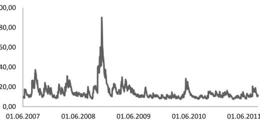
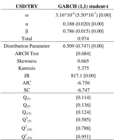
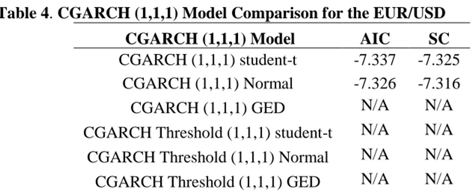
Giray Gozgor ________________________________________________________________ ht h1,t (1 )h2,t (12a) 2 1,t 1 t 1 (1 1) 1, 1t h     h  (12b) 2 2,t 2 t1 2 2, 1t h    _ h _ (12c) At this point, it is important to note that the autocorrelation analyses of the USD/TRY and the EUR/USD exchange rates are carried out in the GARCH and the CGARCH models. We report the Q and the LM tests in order to show results for autocorrelation, and also the Q2 statistics for the accuracy of the variance specification. We use the ARCH-LM tests in order to test the ARCH effect of the lags of variance in the variance equation. We determine the suitable GARCH (p,q) model by the AIC and the SC. We report all results of the model comparison in GARCH (1,1) and CGARCH (1,1,1) in Table 2 for the USD/TRY and in Table 4 for the EUR/USD, respectively. We illustrate the annualized volatility values for the USD/TRY in Figure 1, and for the EUR/USD in Figure 2. We report the GARCH (1,1) and the CGARCH (1,1,1) model features for the USD/TRY and the EUR/USD in Table 3 and Table 5, respectively.

Table 2. Results of the GARCH (1,1) Model Comparison for the USD/TRY GARCH (1,1) Model AIC SC

GARCH (1,1) student-t -6.756 -6.747 GARCH (1,1) Normal -6.705 -6.699 GARCH (1,1) GED -6.747 -6.738

Notes: We sequentially calculate 45 GARCH (p,q) models from GARCH (0,1) to GARCH

(3,3). However, we report the GARCH (1,1) models and select the best model by the AIC and the SC.

Figure 1. The USD/TRY Annualized Volatility

0,00 20,00 40,00 60,00 80,00 100,00 01.06.2007 01.06.2008 01.06.2009 01.06.2010 01.06.2011

(11)

___________________________________________________________ Table 3. The GARCH (1,1) Model Features for the USD/TRY

USD/TRY GARCH (1,1) student-t ω 3.16*10-6 (5.50*10-7) [0.00] α 0.188 (0.020) [0.00] β 0.786 (0.015) [0.00] Total 0.974 Distribution Parameter 6.509 (0.747) [0.00] ARCH Test [0.684] Skewness 0.665 Kurtosis 5.375 JB 817.1 [0.00] AIC -6.756 SC -6.747 Q(5) [0.114] Q(5) [0.136] Q(15) [0.124] Q2(5) [0.585] Q2(10) [0.788] Q2(15) [0.951]

Notes: Standard errors in () and probability values in [ ]. The JB values show the results of

the Jarque-Bera test for normal distribution. As it suggested by Engel (2001), we report the Q and the Q2 statistics up to 15 lags. We use the robust standard errors of Bollerslev- Wooldridge in the normal distribution.

Figure 2. The EUR/USD Annualized Volatility (%)

0,00 5,00 10,00 15,00 20,00 25,00 01.06.2007 01.06.2008 01.06.2009 01.06.2010 01.06.2011

(12)

Giray Gozgor

________________________________________________________________ Table 4. CGARCH (1,1,1) Model Comparison for the EUR/USD

CGARCH (1,1,1) Model AIC SC

CGARCH (1,1,1) student-t -7.337 -7.325 CGARCH (1,1,1) Normal -7.326 -7.316

CGARCH (1,1,1) GED N/A N/A

CGARCH Threshold (1,1,1) student-t N/A N/A CGARCH Threshold (1,1,1) Normal N/A N/A CGARCH Threshold (1,1,1) GED N/A N/A

Notes: We sequentially calculate 45 CGARCH (p,q,r) models from CGARCH (1,0,0) to

GARCH (1,3,3). However, we report the CGARCH (1,1,1) models and select the best model by the AIC and the SC.

Table 5. CGARCH (1,1,1) Model Features for the EUR/USD EUR/USD CGARCH (1,1) student-t

κ 4.81*10-5 (1.75*10-5) [0.006] ρ 0.996 (0.002) [0.00] η 0.034 (0.005) [0.00] α -0.048 (0.012) [0.00] β 0.571 (0.015) [0.016] Distribution Parameter 11.37 (2.227) [0.00] ARCH Test [0.993] Skewness 0.024 Kurtosis 3.676 JB 60.91 AIC -7.337 SC -7.325 QQ(5) [0.280] QQ(5) [0.536] QQ(15) [0.487] QQ2(5) [0.763] QQ2(10) [0.561] QQ2(15) [0.646]

Notes: Standard errors in () and probability values in [ ]. The JB show the results of the

(13)

___________________________________________________________

Now, we can move on the empirical findings that obtained from exchange rate forecasting methodology and the robustness check of our findings.

Comparing Forecast Errors:

We also use the forecasting errors statistics for a comparison of forecasting errors with realized values, regardless of the different sign and scale. We use forecasting errors statistics of the Mean Square Percentage Error (MSPE), and the Mean Absolute Error (MAE). In a comparison of models’ forecasting, the lower MSPE and MAE values indicate that more accurate model. These commonly using forecasting error statistics are simply defined as follows (Poon, 2005: 24):

MSPE= 2 1 1 1 1 _ˆ ( ) N N t t t t t N   N     



(13) MAE= 1 1 1 1 ˆ N N t t t t t N   N     



(14) At this point, Diebold and Mariano (1995) and West (1996) (henceforth the DMW) proposed the t-test to determine whether there is significant difference between the related forecasting errors in two models, and they defined it as follows: H0: 12220 H1: 12220 ( 2 2 1 2 0    or 2 2 1 2 0    )

According to this, test one model (in this study Random Walk model) is considered to be benchmark model. Accordingly, this benchmark models’ MSPE values are calculated as follows:

12 P 1 (yt i)2 







(15)

On the other hand, the MSPE value of the second model subject to comparison with the benchmark model is calculated as follows:

2 1 2 2 P (yt i yˆt i)     





(16)

It is important to note that y_{t i}_ denotes the standard deviation of the benchmark model, whereas y_{t i}_ yˆ_{t i}_ shows the deviation of the second model subject to comparison.Pis the number of observations. Diebold and Mariano (1995) and

West (1996) developed the simple t-test in order to compare the performances of the benchmark model with other models. According to this, while the null hypothesis shows that the performances of both of models are equal, an alternative

(14)

Giray Gozgor

________________________________________________________________ hypothesis shows that the other models are less or more accurate than the benchmark model. If they contain less forecasting errors that means they will have significant positive DMW test statistics. Accordingly, the DMW test statistic is simply defined as follows:

1 f DMW P V 

(17)

f yt i (yt i yˆt i)

(18)

1 f P



f and 1 2 ( ) V P



f

(19)

Now, we can move on the empirical results of the related methodology.

3. Empirical Results

We apply the methodology in the related forecasting models and methods, and compare the recursive scheme out-of-sample forecasting errors by using the DMW test. We report that the MSPE and the DMW test statistics for the USD/TRY and the EUR/USD exchange rates in different periods as the performance analyses in Tables 6, 7 and 8.

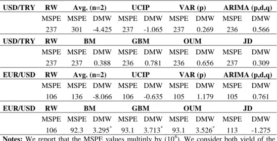
Table 6. Performance Analysis of the USD/TRY and the EUR/USD (June 1, 2007-August 31, 2011)

Notes: We report that the MSPE values multiply by (106). We consider both yield of the government bonds and the policy rates of central banks in the UCIP and the VAR (p) models, and report the minimum MSPE values among them. The DMW test table values at 10%, 5% and 1% are 1.32, 1.72 and 2.51, respectively. * indicates the better performance exists at the 1% significance level.

USD/TRY RW Avg. (n=2) UCIP VAR (p) ARIMA (p,d,q)

MSPE MSPE DMW MSPE DMW MSPE DMW MSPE DMW

237 301 -4.425 237 -1.065 237 0.269 236 0.566

USD/TRY RW BM GBM OUM JD

237 237 0.388 236 0.781 236 0.656 237 0.309

EUR/USD RW Avg. (n=2) UCIP VAR (p) ARIMA (p,d,q)

106 136 -8.066 106 -0.635 105 1.179 105 0.761

EUR/USD RW BM GBM OUM JD

(15)

___________________________________________________________

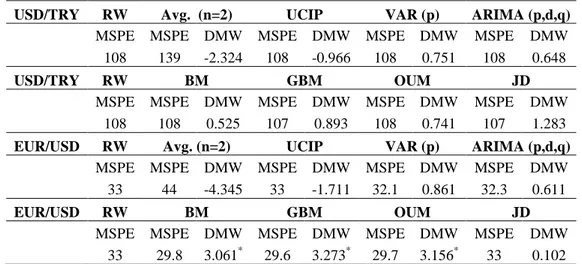
Table 7. Performance Analysis of the USD/TRY and the EUR/USD (July 1, 2008-February 1, 2009)

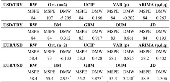
Empirical evidences in Tables 6, 7, and 8 suggest that no model or process can continuously and significantly outperforms the random walk model for the USD/TRY. However, when whole sample and post-crisis period is considered, the minimum MSPE values are provided by GBM and OUM processes for the USD/TRY. On the other hand, JD process is relatively well-performed in the crisis period. Empirical findings from our performance analyses also suggest that GBM, BM, and OUM stochastic processes can continuously and significantly outperform the random walk model for the EUR/USD. These results are all valid in the whole sample, crisis period and post-crisis period for the EUR/USD exchange rate. Empirical findings of the USD/TRY and the EUR/USD predictability can be directly drawn in Tables 6, 7, and 8, and they can easily be interpreted. However, we would like to discuss some findings that seem to be stayed in the background. For example, the first fact may be the power of the DMW test. The DMW and similar predictive ability tests have widely been discussed in the literature. Generally, the DMW test has basically been criticized by the proposition that the t-student distribution table values of this test are oriented to rejection for the hypothesis of “nominal exchange rates are predictable” (Della Corte and Tsiakas 2012). However, excluding the results of JD process for the USD/TRY in the crisis period, our main findings are quite obvious. One can only argue that results of JD process for the USD/TRY in the crisis period can be significant at 10% level; USD/TRY RW Avg. (n=2) UCIP VAR (p) ARIMA (p,d,q)

108 139 -2.324 108 -0.966 108 0.751 108 0.648

108 108 0.525 107 0.893 108 0.741 107 1.283

EUR/USD RW Avg. (n=2) UCIP VAR (p) ARIMA (p,d,q)

33 44 -4.345 33 -1.711 32.1 0.861 32.3 0.611

(16)

Giray Gozgor

________________________________________________________________ however, this will only state the “weak significance level” for exchange rate predictability. Following Della Corte and Tsiakas (2012)10, we can assert that the failure predictability for the USD/TRY is not occurred by the possible lack of power of the DMW test. Secondly, our findings also suggest that the USD/TRY exchange rate market is more volatile and fat-tailed than the EUR/USD.11

Table 8. Performance Analysis of the USD/TRY and the EUR/USD (February 1, 2009-August 31, 2011)

4. Robustness Check

In this paper as far as possible, we try to avoid from all kinds of “intrinsic motivators” or in a broad sense, to avoid any factor that may be related into “behavioral economics” or “behavioral finance”. Thus we attempt to define a “mechanical methodology”. Beyond any doubt, not only subjectivity of researchers and “animal instinct” behaving of market agents, but also parameters of “news effect” and “market expectations” can be incorporated into our stochastic processes methodology or they can theoretically be modeled. Confirmation of the Meese and Rogoff’s findings by numerous empirical studies has led to the judgment that

10_{They have recently argued that the model selection criteria based upon statistical,} economic and econometric evolutions.

11

Out-of sample forecasted annualized average GARCH volatility is 15.79% for the USD/TRY and 10.14 % for the EUR/USD in whole data sample. In the forecasting period, average GARCH volatility is 14.62% for the USD/TRY and 11.15 % for the EUR/USD. All these results are available upon request.

USD/TRY RW Ort. (n=2) UCIP VAR (p) ARIMA (p,d,q)

84 107 -5.205 84 0.166 84 -0.202 84 0.263

84 84 0.312 83 0.917 83 0.861 84 0.193

EUR/USD RW Ort. (n=2) UCIP VAR (p) ARIMA (p,d,q)

58.4 73 -6.133 58.3 0.428 58.1 0.825 58.2 0.402

(17)

___________________________________________________________

nominal exchange rates almost follow a martingale difference sequence. In other words, future changes in nominal exchange rates are unpredictable when they base upon past changes. This definition of martingale behavior is consistent with “weak-form market efficiency” in foreign exchange markets (Yang et al. 2008). Fundamental methods in exchange rate predictability generally focus on serial correlation (or white noise) properties, rather than martingale difference. However, from a nonlinear time series perspective, we know that there is a considerable difference between serial correlation (and white noise) and a martingale difference sequence. Nonlinear time series can have zero autocorrelation, but have a non-zero conditional mean that based on its past history, which implies “predictable nonlinearity” in mean. Thus, when one applied the nonlinear time series by fundamental exchange rate predictability methods, they could yield a result of distortion in favor of the martingale hypothesis (Hsieh, 1993).

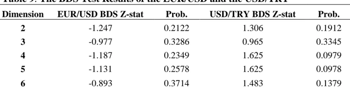
We basically suggest that OUM stochastic process and/or GARCH type volatility models are capable to model the possible nonlinearity in our data. However, we apply the BDS test of Brock et al. (1996) for possible misspecification in the return of exchange rates, and report the BDS test results for the EUR/USD and the USD/TRY in Table 9 as follows:

Table 9. The BDS Test Results of the EUR/USD and the USD/TRY

Dimension EUR/USD BDS Z-stat Prob. USD/TRY BDS Z-stat Prob.

2 -1.247 0.2122 1.306 0.1912

3 -0.977 0.3286 0.965 0.3345

4 -1.187 0.2349 1.625 0.0979

5 -1.131 0.2578 1.625 0.0978

6 -0.893 0.3714 1.483 0.1379

Notes: The table shows the BDS test results in which obtained from standardized residuals

in related GARCH models for the EUR/USD and the USD/TRY. According to the null hypothesis of the test, residuals are independent and identically distributed. Rawvalues are based upon the pairs of friction method and related values are 1.434 for the EUR/USD and 1.386 for the USD/TRY.

Following the results of the BDS test in Table 9, we can assert that a possible presence of nonlinearity is also captured by our methodology. We now suggest that ‘the predictability success’ in the results of the EUR/USD, and the “the predictability failure’ in the results of the USD/TRY can simply and mainly explained by the efficient-market hypothesis. The EUR/USD exchange rate market is unquestionably more efficient than the USD/TRY exchange rate market. We discuss reasons of these general conclusions in the concluding remarks.

(18)

Giray Gozgor

________________________________________________________________ 5. Concluding Remarks

Predictability of nominal exchange rates has become more complicated due to not only the invention of new financial models, instruments and products, but also developments in financial information and technologies. During last decades, exchange rate forecasting methods have transformed from basic linear models into more dynamic techniques. During this transformation process, developments in both time series models and fundamental approaches have led to non-negligible advancements in the exchange rate forecasting literature. In this study we investigate the short-time exchange rate predictability in a developed and in an emerging market and for this purpose consider the EUR/USD and the USD/TRY exchange rates. We apply the benchmark test and compare the results of daily out-of-sample forecasting by four stochastic processes, VAR, ARIMA and UCIP models against the naive random walk. We conclude that martingale difference hypothesis is valid in the USD/TRY exchange rate. In other words, our robust out-of-sample forecasting results for the USD/TRY cannot reject the applicability of the “exchange rate disconnect puzzle” or the “Meese-Rogoff puzzle”. However, we are able to reject the validity of the “Meese-Rogoff puzzle” for the EUR/USD. Furthermore, we show that these findings are robust and not time-specific. When we separately examine the pre-crisis and the post-crisis periods, results remain unchanged. We therefore basically suggest that findings of ‘predictability success’ in the EUR/USD can mainly be explained by the fact that the EUR/USD exchange rate market is in more “efficient-form” than the USD/TRY exchange rate market, due to a martingale behavior in asset price is strongly consistent with weak-form market efficiency in any foreign exchange market.

We think that this general inference of market efficiency can be explained by several facts or reasons. First, the USD/TRY exchange rate market is more vulnerable than the EUR/USD exchange rate market, particularly in the periods of global imbalances. This also can be shown by the results of higher GARCH volatility in the USD/TRY yields. Second, we can call the USD/TRY exchange rate market as the “semi-organized loose oligopoly” market. It can be said that banks are most crucial agents in the USD/TRY exchange rate market. When we even consider that every bank has an “exchange rate investment position”, and so an “exchange rate level expectation”, we can easily suggest that a remarkable reason of unpredictability is the “lack-of-deepness” in the USD/TRY exchange rate market. Third, in the “relatively smaller ”financial markets like the USD/TRY exchange rate market an approach that can be defined as “uncertainty-oriented” is the main determinant factor, probably much the same in all financial markets. As we have already mentioned, the EUR/USD trades at a “global” and an “organized” market; however the USD/TRY trades at a “local” and a “semi-organized” market. Similarly, derivatives markets and instruments are also more developed and more complicated for the EUR/USD exchange rate. Thus, we would like to emphasize that a kind of “uncertainty-oriented” approach is also an important factor on banks’ investment position in the USD/TRY exchange rate market. Fourth, whatever exchange rate regime is implemented in an open-economy, values of nominal

(19)

___________________________________________________________

exchange rates are certainly a monetary policy tool. It can be said that values nominal exchange rates have significant direct or indirect effects on monetary policy and/or on the results of monetary policy. Because of this, it is certainly “suspicious” and “controversial” issue whether the actual market value in foreign exchange markets shows that an “equilibrium price” at any time, particularly in emerging market economies. When we consider the issue in terms of the USD/TRY exchange rate market, the CBRT has not only randomly, but also “systematically” intervened to the USD/TRY exchange rate market. At this point, effects of “reserve currency shortage” or “reserve currency constraint” should not be ignored in Central Banks’ interventions into foreign exchange markets.

Of course, the empirical findings of out-of-sample predictability success in stochastic processes for the EUR/USD in this study, is not only important for researchers that using the fundamental-based approaches, but also market agents in the terms of using technical trading models. Empirical results in this paper indicate that stochastic processes should more extensively be used in the exchange rate forecasting literature. Nevertheless, within the framework of the methodology described in this paper and forecasts arise from related stochastic processes are not the ‘armada invincible’ even for the EUR/USD. Stochastic processes and their methodology described in this paper are still open fields, particularly associated with “behavioral economics” and “behavioral finance”. Additionally, it is always possible to achieve results of better significant performance than random walk model in exchange rate predictability by using stochastic processes, as well as following a different methodology that used in this study.

Future studies will be built on the exchange rate predictability by using stochastic processes can be applied into a greater number of developed and developing exchange rate markets, in order to provide results and inferences in above can be seen as “more general state” in literature. Similarly, using weekly, monthly or different frequency data by a methodology within stochastic processes, one can perform short-term, medium-term and long-term exchange rate predictability.

REFERENCES

[1]Achelis, S.B. (2003), Technical Analysis from A to Z; Equis International, Salt Lake City;

[2] Bollerslev, T. (1986), Generalized Autoregressive Conditional Heteroskedasticity; Journal of Econometrics, Vol. 31, pp. 307-328;

[3] Brigo, D., Dalessandro, A., Neugebauer, M., Triki, F. (2009a), A Stochastic Process Toolkit for Risk Management: Geometric Brownian Motion, Jumps, GARCH and Variance Gamma Models; Journal of Risk Management in Financial Institutions, Vol. 2, pp. 365-393;

(20)

Giray Gozgor

________________________________________________________________ [4] Brigo, D., Dalessandro, A., Neugebauer, M., Triki, F. (2009b), A Stochastic Process Toolkit for Risk Management: Mean Reverting Processes and Jumps; Journal of Risk Management in Financial Institutions, Vol. 3, pp. 65-83;

[5] Brock, W.A., Dechert, D.W., Scheinkman, J.A., LeBaron, B. (1996), A Test for Independence Based on the Correlation Dimension; Econometric Reviews, Vol. 15, pp. 197-235;

[6]Cheung, Y.W., Chinn, M.D., Pascual, A.C. (2005), Empirical Exchange Rate Models of the Nineties: Are Any Fit to Survive?, Journal of International Money and Finance, Vol. 24, pp. 1150-1175;

[7]Chongcheul, C., Kim, Y., Yoon, S. (2012), Can We Predict Exchange Rate Movements at Short Horizons?, Journal of Forecasting, Vol. 31, pp. 565-579; [8]Corte, P.D., Tsiakas, I. (2012), Statistical and Economic Methods for Evaluating Exchange Rate Predictability; Handbook of Exchange Rates, John Wiley, London, pp. 239-282;

[9]Diebold, F.X., Mariano, R.S. (1995), Comparing Predictive Accuracy, Journal of Business and Economic Statistics ; Vol. 13, pp. 253-263;

[10]Ding, Z., Granger, C.W.J. (1996), Modelling Volatility Persistence of Speculative Returns: A New Approach ;Journal of Econometrics, Vol. 73, pp. 185-215;

[11]Engel, C., West, K.D. (2005), Exchange Rate and Fundamentals; Journal of Political Economy, Vol. 113, pp. 485-517;

[12]Engel, C., Mark, N.C., West, K.D. (2008), Exchange Rate Models are not as Bad as you Think; National Bureau of Economic Research Macroeconomics Annual, Vol. 22, University of Chicago Press, Chicago, pp. 381-441;

[13]Engle, R.F. (2001), GARCH 101: The Use of ARCH/GARCH Models in Applied Econometrics ;Journal of Economic Perspective, Vol. 15, pp. 157-168; [14]Fratzscher, M. (2009), What Explains Global Exchange Rate Movements during the Financial Crisis?, Journal of International Money and Finance, Vol. 28, pp. 1390-1407;

[15]Hansen, P.R., Lunde, A. (2005), A Forecast Comparison of Volatility Models: Does Anything Beat a GARCH (1,1)? Journal of Applied Econometrics, Vol. 20, pp. 873-889;

[16]Hsieh, D.A. (1993), Implications of Nonlinear Dynamics for Financial Risk Management ;Journal of Financial and Quantitative Analysis, Vol. 28, pp. 41-64; [17]Mark, N.C. (1995), Exchange Rates and Fundamentals: Evidence on Long-Horizon Predictability ; American Economic Review, Vol. 85, pp. 201-218; [18]Meese, R.A., Rogoff, K.S. (1983a), Empirical Exchange Rate Models of the Seventies: Do They Fit Out of Sample? Journal of International Economics, Vol. 14, pp. 3-24;

[19]Meese, R.A., Rogoff, K.S. (1983b), The Out of Sample Failure of Empirical Exchange Model ;, Exchange Rates and International Macroeconomics,

(21)

___________________________________________________________

[20]Neely, C.J. (2009), Forecasting Foreign Exchange Volatility: Why is Implied Volatility Biased and Inefficient? And Does It Matter? Journal of International Financial Markets, Institutions and Money, Vol. 19, pp. 188-205;

[21]Poon, S. (2005), A Practical Guide for Forecasting Financial Market Volatility ; John Wiley and Sons, West Sussex;

[22]Rogoff, K.S. (2008), Comment on Exchange Rate Models are not as Bad as You Think ;National Bureau of Economic Research Macroeconomics Annual, Vol. 22, University of Chicago Press, Chicago, pp. 443-452;

[23]Rossi, B. (2013), Exchange Rate Predictability; Journal of Economic Literature, forthcoming;

[24]Schwartz, E.S. (1997), The Stochastic Behaviour of Commodity Price: Implications for Valuation and Hedging ;Journal of Finance, Vol. 52, pp. 923-973;

[25]Wang, Z., Zhong, S. (2009), Application Continuous Time Markov Process to Forecast Exchange Rate; The Proceeding of International Joint Conference on Artificial Intelligence, Hainan Island, China, PR., April 25-26, 2009, pp. 63-66; [26]West, K.D. (1996), Asymptotic Inference about Predictive Ability; Econometrica, Vol. 64, pp. 1067-1084;

[27]Yang, J., Su, X., Kolari, J.W. (2008), Do Euro Exchange Rates Follow a Martingale? Some Out-of-sample Evidence ; Journal of Banking and Finance, Vol. 32, pp. 729-740.

(22)

Giray Gozgor

________________________________________________________________ Appendix I. Simulation Examples of Stochastic Process for Exchange Rate

Forecasting

A Brownian Motion Process for the USD/TRY and the EUR/USD Forecasting

A Geometric Brownian Motion Process for the USD/TRY and the EUR/USD Forecasting

A Mean-reversion Process for the USD/TRY and the EUR/USD Forecasting