W ií'é - W“ * — ta w· ;■ Γ-. / > ‘‘Г · ‘*-··| · · ^ ^ A L S 'D .-'ÎV K i-'jî - ù K iP '5 'C r 2 Н У :^£ :
. / г ^ ^', , :
ti tz ц! U ^4^ ί» ύχΐ.'ϋ ti : ►;> 5 ίτ-:.s г.ѵ^ ;■■“ьх*'··ν * с . ч ’. ·· ■·?*■ ' ^ ’*
I M P L E iV I E N T A T I O N O F T H E B A C K P R O P A G A T I O N A L G O R I T H M O N i P S C / 2 H Y P E R C U B E
M U L T I C O M P U T E R S Y S T E M
A THESIS SUBMITTED TO THE DEPARTMENT OF
COM PUTER ENGINEERING AND INFORMATION SCIENCE AND
THE INSTITUTE OF ENGINEERING AND SCIENCES OF
BILKENT UNIVERSITY
IN PARTIAL FULFILLMENT OF THE REQUIREMENTS FOR THE DEGREE OF
M ASTER OF SCIENCE
By
Deniz Erco§kiin
December 1990
__— tarafisdaa k r : ,L - 'Я й 'H /:
.из
■ 4 3 ^ 0
ÔUB3V
I certify that [ have rearl this thesis and that in rny opinion it is fully adequate, in scope and in quality, as a thesis for the degree of Master of Science.LAX V J ^ X X .tl.X X , t-XvJ U .X X V ^ v J4 v J X W X U
x J k ^
Assist. Prof. Dr. Kemal Of lazer(Principal Advisor)
I certify that I have read this thesis and that in my opinion it is fully adequate, in scope and in quality, as a thesis for the degree of Master of Science.
Assoc. Prof. Dr. Varol xA.kman
I certify that I have read this thesis and that in my opinion it is fully adequate, in scope and in quality, as a thesis for the degree of Master of Science.
Assist. Prof. Dr. Cevdet Aykanat
I certify that I have read this thesis and that in my opinion it is fully adequate, in scope and in quality, as a thesis for the degree of Master of Science.
Assist.' Prof. Dr. Uğur Halıcı
I certify that I have read this thesis and that in my opinion it is fully adequate, in scope and in quality, as a thesis for the degree of Master of Science.
^ J / ) P U
rof. Dr. Neşe Yalabık
Approved for the Institute of Engineering and Sciences:
Prof. Dr. MeliK^t Baray
A B S T R A C T
IMPLEMENTATION OF THE BACKPROPAGATION
ALGORITHM ON iPSC/2 HYPERCUBE
MULTICOMPUTER SYSTEM
Deniz Ercoşkıın
M.S. in Computer Engineering and Information Science
Supervisor; Assist. Prof. Dr. Kemal Of lazer
December 1990
Backpropagation is a supervised learning procedure for a class of artificial neural networks. It has recently been widely used in training such neural networks to perform relatively nontrivial tasks like text-to-speech conversion or autonomous land vehicle control. However, the slow rate of convergence of the basic backpropagation algorithm has limited its application to rather small networks since the computational requirements grow significantly as the network size grows. This thesis work presents a parallel implementation of the backpropagation learning algorithm on a hypercube multicomputer system. The main motivation for this implementation is the construction of a parallel training and simulation utility for such networks, so that larger neural network applications can be experimented with.
Ö Z E T
GERİ YANSITMA ALGORİTMASININ İPSC/2
HYPERCUBE PARALEL İŞLEMCİSİNDE
GERÇEKLEŞTİRİLMESİ
Deniz Ercoşkım
Bilgisayar ve Enformatik Mühendisliği Yüksek Lisans
Tez Yöneticisi: Y. Doç. Dr. Kemal Of lazer
Tarih 1990
Geri yansıtma, bazı yapay sinir ağı modelleri için geliştirilmiş bir öğrenme al goritmasıdır. Bu algoritma, özellikle bu tip sinir ağı modellerinin eğitilmesinde kullanılmaktadır. Temel geri yansıtma algoritmasının yavaş yakınsaması bu algoritmanın kullanımını küçük sinir ağlarıyla sınırlandırmıştır. Bu tez çalış masında geri yasıtma algoritması hypercube paralel işlemcisinde gerçekleştirilmiş ve bir dizi yapay sinir ağına uygulanmıştır. Bu çalışmanın diğer bir amacı, buyuk yapay sinir ağları için bir simulasyon ve öğretim ortamı geliştirilmesidir.
A C K N O W L E D G iM E N T
I thank my advisor, Assist. Prof. Dr. Kernal Oflazer for teaching me the meaning of the word “research,” and providing perfect dosage of criticism and unfailing support throughout the thesis. I am thankful for his proper combina tion of justice and mercy on deadlines to ensure the completion of this thesis. I explicitly want to acknowledge the helpful contributions of Assist. Prof. Dr. Cevdet Aykanat during the last stages of my work. I owe debts of gratitude, to Elvan Göçmen, Zeliha Gökmenoğlu, Güliz Ercoşkun, Müjdat Pakkan for their help in shaping this thesis. Finally, I owe a measure of gratitude Bilkent University, who provided a very fruitful environment without which this work could not have been possible.
Contents
1 In tro d u c tio n
2 A rtificia l N eu ra l N etw o rk s
3 P e r c e p tr o n s
3.1 Single Layer P erceptrons... 7
3.2 Multilayer P e rce p tro n s... 9
3.2.1 Backpropagation Networks 4 T h e B a ck p r o p a g a tio n A lg o r ith m 11 5 P a r a lle l Im p le m e n ta tio n o f B a ck p r o p a g a tio n A lg o r ith m 16 5.1 Parallelism in Backpropagation ... 16
5.2 The Hypercube A rchitecture... 17
5.3 Mapping Backpropagation to H y p e rcu b e ... 18
5.4 Other Parallel Im plem entations... 22
6 H Y P E R B P - T h e P a ra llel B a ck p r o p a g a tio n S im u la to r 24 6.1 Backpropagation Block Delimiter C a l l s ... 25
6.2 Neural Network Definition Calls 26
CONTENTS ^jj
6.3 Training Parameters Setting C a lls ... 30
6.4 Training Set Specification Calls 31 6..5 Neural Network Simulation Calls 34 6.6 Neural Network Training C a l l ... 33
6.7 Information Retrieval C a lls... 35
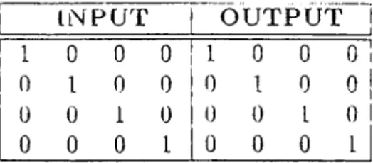
6.8 Scimple Program 4-2-4 Encoding/Decocling P ro b lem ... 38
7 P erfo rm an ce M odels for th e S im u lato r 42 7.1 Parameters of the Mathematical M o d e l... 42
7.1.1 System Param eters... 43
7.1.2 Problem P a r a m e te r s ... 45
7.2 Model for Network Partitioning Off-line... 45
7.3 Model for Training Set Partitioning O f f - lin e ... 47
8 E x p erim e n ts 8.1 8 Bit Parity P ro b le m ... 49
8.1.1 Problem D e sc rip tio n ... 49
8.1.2 Backpropagation Approach ... 50
8.2 Digit Recognition P ro b le m ... 52
8.2.1 Problem D e sc rip tio n ... 52
8.2.2 Backpropagation Approach ... 53
8.3 The Two Spirals Problem ... 55
8.3.1 Problem D e sc rip tio n ... 55
CONTENTS V lU··;
S.-t NETTalk ... 5g 5.4.1 Problem D e scrip tio n ... 53
8.4.2 Backpropagation Approach 53
9 C onclusions 03
A D eriv atio n of th e B ack p ro p ag atio n A lg o rith m 65 A. I Backpropagation R u l e ... 55 A.2 The Derivation of Backpropagation R u l e ... 55
L ist o f F ig u r e s
2.1 Artificial Neural Network M o d el... 5
3.1 A Single-Layer P e rc e p tro n ... 8
3.2 A Backpropagation Neural N etw ork... 10
4.1 A Backpropagation Neural N etw ork... 12
5.1 Mapping backpropagation to multiple processors using Network P a rtitio n in g ... 19
5.2 Partitioning the weight matrix for forward and backward passes... 21
5.3 Mapping backpropagation to multiple processors using Training Set P a rtitio n in g ... 22
8.1 A subset of the training set of 8 Bit Parity P roblem ... 51
8.2 Number of processors versus speed up graph for 8 bit parity p r o b le m ... 53
8.3 Number of processors versus speed up graph for digit recognition p r o b le m ... 54
8.4 Training points for two-spirals p ro b le m ... 55
8.5 Fragment of C code which generates the training set of two-spirals p r o b le m ... 56
LIST OF FIGURES x
8.fS iN'trnbT of pror<^ssors versus speed up ¿^raph for two-spirals prob lem ... 5S 8.7 Prescritatiou of word competition to NETtalk Mcural Network 60 8.8 Number of processors versus speed up graph for NETTalk problem 61
L ist o f T a b les
6.1 The table illustrating 4-2-4 Encoding Decoding Problem .38
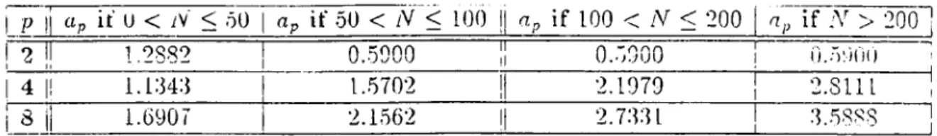
7.1 flp values used in the calculation of 44
7.2 bp values used in the calculation of 44
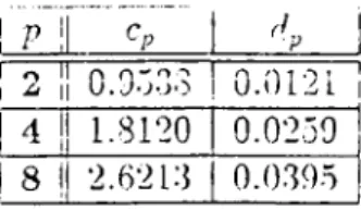
7.3 Cp, dp values used in the calculation of ... 45
8.1 Results for 8 Bit Parity Problem (Times are per epoch and in se c o n d s)... 52 8.2 Results for digit recognition network (Times are per epoch and
in seconds)... 54 8.3 Results for two-spirals network (Times are per epoch and in
se c o n d s)... 57 8.4 Results of NETTalk problem (Times are per epoch and in seconds) 61
C h a p te r 1
Introduction
Backpropagation [22] is a supervised learning procedure for a class of artificial neural networks. It has recently been widely used in training such neural net works to perform relatively nontrivial tasks (e.g., text-to-speech conversion [27], autonomous land vehicle control [16]). However, the slow rate of convergence of the basic backpropagation algorithm coupled with the substantial computa tional requirements has limited its application to rather small networks. In this thesis, a parallel implementation of the backpropagation learning algorithm on an 8-processor Intel iPSC/2 hypercube multicomputer system is presented.
In computer science, there is a widespread feeling that conventional com puters are not good models of the cognitive processes embodied in the brain. Tasks like arithmetic calculations and flawless memorization of large numbers of unrelated items are very easy for the computers and very hard for humans. However, humans are much better than computers at recognizing objects and their relationships, at natural language understanding, and at commonsense reasoning. In addition to all these, humans are experts at learning to do things through experience. The computational process in the brain is significantly different from those in the computers, and this causes the performance differ ence between humans and computers. The human brain consists of billions of comparatively slow neurons, that all compute in parallel, while conventional digital computers have fast processor units, which operate by executing in a sequential manner a sequence of very simple primitive steps [7].
The Artificial Neural Network model is a computational model proposed for emulating the functionality of human brains. This model consists of many
Chapter L Introduction
iieurou-iike computaciotial elements operatin':; in parallel, arranged in a striir-turc :similar to biological neural networks [13]. Learning, a property a,ssodar,ed only with humans and animals, is a very important property of this model [1].
Artificial neural networks has been a popular research area for the last forthy years. During this period a number of different neural net models have been proposed, e.g., Hopfield networks [9], Boltzmann Machines [1], Kohonen’s Self Organizing Feature Maps [13], Perceptrons [20].
The perceptron model was introduced in 1962 [20]. Later a special class of perceptrons multi-layer perceptrons attracted significant attention, mainly because of its simple structure, and potential capacity. Learning algorithm, called the backpropagation learning algorithm for a subclass of multi-layer per ceptrons was proposed in 1986 to solve the learning problem of multi-layer perceptrons [23]. This thesis presents a tool for training and simulating back- propagation neural networks on an Intel’s iPSC/2 hypercube multicomputer system. The main motivation for this implementation is the development of a parallel training and simulation utility for this class of networks so that larger neural network applications can be experimented with.
The remaining parts of this thesis are organized as follows. Chapter 2 surveys artificial neural networks. In Chapter 3, the two classes of percep trons, namely single-layer and multi-layer perceptrons, and a subclass of multi layer perceptrons called backpropagation neural networks are explained in de tail along with their network topologies and the applicable learning algorithms. Chapter 4 gives a detailed explanation of the standard backpropagation learn ing algorithm. Chapter 5 discusses the parallelism in the backpropagation algorithm and presents general information about the iPSC/2 system. Af terwards, the implementation of the standard backpropagation algorithm on the Intel iPSC/2 Hypercube multicomputer system is explained, along with the detailed explanation of two different approaches to the algorithm, network partitioning and training set partitioning. Finally, other parallel implemen tations of the backpropagation algorithm in literature along with the perfor mance achieved with these implementations and the parallel platforms used are summarized. Chapter 6 describes our parallel backpropagation training and simulation tool, HYPERBP. Chapter 7 gives mathematical performance
Chapter 1. Introduction
models tor calculatint^ the theoretiral elao'^ed times of network partitioning oiT- linc, and tralaiiig set partitioniini; oiT-line approaches. By applying tlie neiiral network problem parameters to the models, a user can estimate tlie elapsed times of these approaches, and can select the appropriate approach for a neural network problem without actually running it on the multicomputer. Chapter 8 discusses the five neural networks that are experimented with, using the HY PERBP. The problem descriptions, parameters, experimental results as well as the theoretical results calculated using the mathematical model, are given in this chapter. Conclusions are given in Chapter 9. Appendix A presents the detailed derivation of the standard backpropagation learning algorithm.
C h a p te r 2
Artificial Neural Networks
Studies for simulating computational processes in brain-like systems brought the need for models of computation that are appropriate for parallel systems composed of large numbers of interconnected, simple units. From these studies a model called Artificial Neural Networks is emerged. Artificial neural networks are referred by many different names in literature: Neural Nets, Connection- ist Models, Parallel Distributed Processing (PDP) models, and Neuromorphic Systems [13]. All these models are composed of many computational elements operating in parallel and arranged in patterns similar to biological neural net works. Artificial neural networks have six major aspects [21]:
1. A set of processing units, 2. a state of activation,
3. a pattern of connectivity among units,
4. a propagation rule for propagating patterns of activities through network of connectivities,
5. an activation rule for combining the inputs impinging on a unit with the current state of the unit to produce a new level of activation for the unit, and
6. a learning rule whereby patterns of connectivity are modified by experi ence.
Chapter 2. Artificial Neural Networks
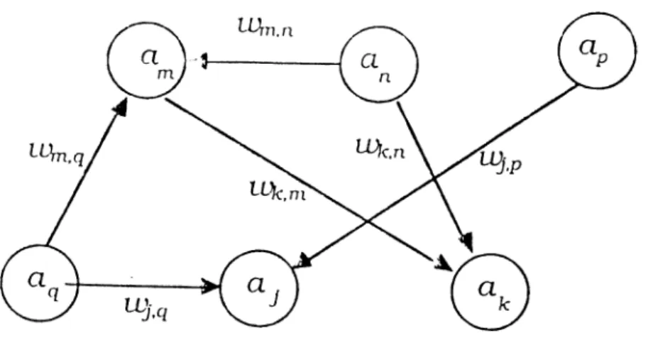
Figure 2.1: Artificial Neural Network Model
An artificial neural network consists of a set of processing units (see Fig ure 2). Every unit in the network has an activation value (denoted by a,·) at each point in time. The units within the neural network are connected to each other. The pattern of connectivity along with the neurons, determine what the response of the network to a specific input, will be. The output value of a unit is sent to other units in the system through this set of unidirectional connections (in Figure 2 the connections are represented as arrows between units). Associated with each connection, is the lueight or the strength of the connection. The weight of a connection from unit i to unit j is represented as Wji, and determines the amount of effect the source unit has on the destination unit. How the incoming inputs to a unit should be combined is determined by a propagation rule. The output values of the source units are combined with the corresponding weight values of the connections. Then, with the help of the propagation rule, the net input of the destination unit is calculated. The activa tion value of a unit is passed through a rule called activation rule to determine the new activation value of the unit. The artificial neural networks are mod ifiable, in the sense that the pattern of connectivity can change as a function of experience. Changing the processing or knowledge structure of an artificial neural network model involves changing the pattern of its connectivity. The rule which defines how weights or strengths of connections should be modified
Chapter 2. Artificicil Neural Networks
lurougii experience is ilermed by the learning rule ot the network, '['his
13 called as learning or training. Learning cnui eillier he supervised where an external agent indiciites to the network what the correct response should be^ or unsupervised where the network itself classifies the input patterns. (See [6] for a detailed overview of various learning methods.)
Artificial neural network models offer an alternative knowledge represen tation paradigm against conventional models. In neural network models the knowledge is represented in a distributed fashion by the strength of connec tions and interactions among numerous very simple processing units. Neural networks also offer fault tolerance. This property of artificial neural networks is mainly due to the distributed representation, since the behavior of the net work is not seriously degraded when a (small) number of processing units fail. Another important property of the artificial neural networks over conventional models is that they can learn their behavior through a training or learning process.
C h a p te r 3
Perceptrons
3,1 Single Layer P ercep tron s
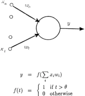
Perceptron is the name given to a class of simple artificial neural network structure [20, 25, 8]. A perceptron is a threshold logic unit with n inputs (see Figure 3.1). Associated with each input there is a real valued weight that plays a role analogous to the synaptic strength of inputs to a biological neuron. The input to the perceptron is an n-dimensional vector. The perceptron multiplies each component of the input vector with the associate weight and sums these products. The perceptron gives an output of 1 if this sum exceeds a threshold value 0 and 0 otherwise. A more formal definition is given in Equation 3.1, where x,· is the activity on the input line and Wi is the associated weight, and 9 is the threshold.
Perceptrons can learn their expected behavior through a process called the Perceptron Convergence Procedure [20]. The procedure is as follows:
1. First, connection weights are initialized to small, random, non-zero val ues.
2. Then, the input with n continuous valued elements is applied to the input and the output is computed using equation 3.1. If the computed output value is different from the desired output value then connection weights are adapted using the error correction formula
Clicipíer Percer)trons
(3.1)
Figure 3.1: A Single-Layer Perceptron
where ojj is the weight of the connection connecting the input value to the perceptron, 77 is a constant which determines the learning rate of the procedure, t is the target (expected) value of the perceptron, o is the calculated value of the perceptron, ij is the input value.
3. Step 2 is repeated until the network responds with the desired outputs to the given inputs.
The main result proven about perceptron convergence procedure is the following: Given an elementary perceptron, an input word W which consists of n continuous elements, and any classification C{W) for which a solution exists, then beginning from an arbitrary initial state, perceptron convergence procedure will always yield a solution to C{W ) in finite time. Thus, if the given classification is separable (that is the classes fall on different sides of some hyperplane in n dimensional space), then the perceptron convergence procedure converges and positions the decision hyperplane between these classes [20, 13].
The results of a very careful mathematical analysis of the perceptron model was published in 1969 [14]. This careful analysis of conditions under which perceptron systems are capable of carrying out the required mapping of input
Chapter 3. Perceptrons
CO oucpuc showed ciia.t in a. large number of interesting rases, rmtv.'ork models of tliis kind aro not capable of solving the pixdslern [14]. This idea was siij^norterl by many example problems, where perceptron models failed to find the solution. A classical example problem is the exclusive-or, (XOR) problem where the output is 0 if the inputs are same, and it is I if they are different. It has been shown that perceptron model fails to solve even such a simple problem [14] because the inputs of the problem is not separable. Thus, the single layer perceptron model can not solve the XOR problem, since there is no hyperplane (a line in this case) to separate the two classes of the problem.
3.2
M u ltilayer P ercep tro n s
Following these pessimistic results, an alternative model was suggested where the perceptron model was augmented with a layer of perceptron-like hidden units between input nodes and original perceptron layer. In such networks, there is always a recording (internal representation) of the input patterns in the hidden units. As a consequence, these hidden units can support any required mapping from input to output units. Thus, if we have the right connections from the input patterns to a large enough set of hidden units, we can always find a representation that will perform any mapping from input to output through these hidden units. This model given the name multi-layer perceptrons [14].
The multi-layer perceptron model fixed all the weaknesses of single-layer perceptrons. However, in spite of its strong features, the multi-layer percep trons had a very important problem: They did not have a provably convergent learning procedure. Perceptron convergence procedure which is applicable to single-layer perceptrons, could not be extended to multi-layer perceptrons, be cause it could not adjust the weights between the perceptrons.
3.2.1
B ackpropagation N etw ork s
The pessimistic results about perceptrons actually halted the research on neural networks for about 20 years. In early 1980’s, several solutions for the learning problem of multi-layer perceptrons were proposed, but none had the guarantee of convergence.
(Jhripter ’L Perceptron^ conn<?ct'ions - - > connections — >
t
t
t
/ hidden units input unitsFigure 3.2: A Backpropagation Neural Network
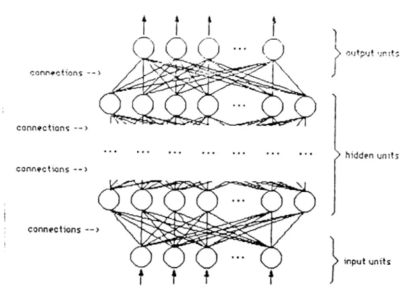
In 1986, a learning procedure for a subclass of multi-layer perceptrons was proposed [24]. This procedure is applicable specifically io fully connected^ layered, feedforward multi-layer perceptrons as shown in Figure 3.2. The proce dure is named the Backpropagation Learning Procedure, and the corresponding subclass of multi-layer perceptrons is generally called as Backpropagation Net
works. In backpropagation networks activations flow from the input layer to the output layer, through a series of hidden layers. Each unit in a layer is connected in the forward direction to each unit in the next higher layer. In backpropagation networks the activation values of the input layer is set in ac cordance with the sample input, then the rest of the units in the network find their activation values. The activation values of the units in the output layer determine the output of the network. The learning rule is called as the back- propagation rule [22], and is in fact a generalization of Perceptron Convergence Procedure. Backpropagation Learning Procedure involves only local computa tions. Although it does not guarantee to converge to the correct solution, in almost all applications it has done so. These properties of the learning algo rithm, and the strong features of the multi-layer perceptron algorithm, made the multi-layer perceptrons a very popular neural network model.
C h a p te r 4
The Backpropagation Algorithm
The backpropagation algorithm is a supervised learning method for the class of networks described in Chapter 3. Starting with a given network structure and weights initialized to small random values, the backpropagation algorithm updates the weights between units as a given set input/output pattern associa tions - known as the training set - are presented to the network. Presentation of all the patterns in the training set to the network is known as an epoch. The backpropagation algorithm can be implemented as either an on-line or an off-line version. In the on-line version, the weights in the networks are ad justed after each input/output pair is presented, while in the off-line method the weights are adjusted after an epoch. The on-line method is described below (the off-line method is very similar).
In on-line training, each input/output presentation consists of two stages: 1. A forward pass during which inputs are presented to the input layer and
the activation values for the hidden and the output layers are computed. 2. A backward pass during which the errors between the computed and ex pected outputs are propagated to the previous layers and the weights between the units are appropriately updated.
Training a backpropagation network typically takes many epochs. The net work weights may never settle into stable values for certain problems as there is no corresponding convergence theorem for this algorithm. However, in prac tice almost all the networks have converged to configurations with reasonable performance.
Chapter 4. The Backpropagation Algorithm 12
o o o o
f
t
t
t
o o o o
2 3 4
Figure 4.1: A Backpropagation Neural Network
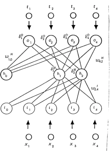
The following is a formal description of the backpropagation algorithm for networks with a single hidden layer - extension to networks with multiple hidden layers is straightforward. Let Ni, Ns and No be the number of units at the input, hidden, and the output layers of a network respectively. We assume that the input and hidden layers employ an additional unit for thresholding purpose whose output is always a 1. The activation values will be denoted by ij (0 < J' < A^,·, ¿0 = 1 always) at the input layer, by hj (0 < j < Nh, ho = 1 always) at the hidden laj'er, and by Oj (1 < i < No), at the output layer. Let the elements of the pattern vector be Xj (1 < i < Ni) and the coriesponding expected output be tj (1 < i < No) (see Figure 4). We initialize the input layer:
7J = X j 1 < ; < A ' . (-1.1)
Chapter k The Backpropagation Algorithm 13
ferzO 1
.2)
which is the weighted sum computation and application of activation function F. In backpropagation learning algorithm generally, the sigmoid function is used as the activation function. The sigmoid function is defined as
F(a) = I (T3)
1 + e-(«)
Then, we propagate the activations from hidden layer to the output layer with
(4.4) k=o
Heveujf. denotes the weight between the input unit and th ey ‘d hidden unit, and denotes the weight between the hidden unit and the output unit. We then compute the errors at the output layer as
8° = Oi{l - - Oi) l < j < N o (4.5) This definition of the error is related to the derivative of the activation function (see Appendix A, for the details of the mathematical derivation.) These errors are then propagated to the hidden layer as
No
(4.6) Jt=l
The weights between the hidden and output layers are then updated with
l < k < N . a < j < N H , (4.7) and the weights between the input and hidden layers are updated with
Aw( · = 1 < < A)i, 1 < i < (4.8) here 7/ is a constant called the learning rate.
^In networks with more than one hidden layer, such errors are computed for every hidden layer.
(Jhripter i. '['he BackpvopngpJion Algoritlun I [
The oiT-Hae version of the algorithm accumulates thc'^e values for nil the patterns during an epoch and peL-forms <i weight update oidv <\i idle end of the epoch with the ¿iccurnulated changes. The computation of may also involve a niomeiitiiiii term in certain implementations of the algorithm ; this has been observed to improve the convergence rate. Using a momentum term o:, the weight update rule for all layers is changed to
A u k j = T]Spij + aA ujlj where j is the previous Auj^j value.
(1.9)
The procedure outlined above is repeated with every iiiput/output pair in the training set and epochs are repeated as many number of times as necessary until satisfactory convergence is achieved (though as stated earlier there is no guarantee for convergence).
A clo ser lo o k at th e forw ard pass
The forward pass of the backpropagation computation is essentially a sequence of matrix - vector multiplications with intervening applications of the sigmoidal activation function to each element of the resulting vectors. For example, the outputs of the first hidden layer H = [hi,h2, . . . , can be written as
H = F(W ^ · I) (4.10)
where denotes the Nh x (A,· + 1) matrix^ of weights between the input and the hidden layers, I denotes the input vector and F denotes the sigmoidal activation function applied to each element of the vector. For the output layer one can similarly write
0 = F’(W “ -H ') (4.11)
where denotes the No x {Nh + 1) weight matrix between the hidden and the output layers and O = [oi,c>2) · · · > is the output vector and H ' is the same as H with ho prepended. It is therefore possible to use parallel algorithms for matrix-vector multiplication for the parallel processing platform available.
Chapter i. The Dackpropagation Algoritlun lo
A cl oser look at the b a c k w a r d pass
During the backward pass, the computed at the output layer are prop¿ı- gated to the previous layers. A closer look at the definition of 6^ shows that the summation involved is actually computing an entry of the multiplication of a matrix (W ^)^ - the transpose of the weight matrix - and the vector
6^ = · · · 7 Each such element computer is then multiplied by a scalar — hi)). Once 6^ is computed, A W ’s can be computed and the weight matrices can be updated.
Parallel Implementation of Backpropagation
Algorithm
C h a p te r 5
5.1 P arallelism in B ackpropagation
The backpropagation algorithm described in Chapter 4 offers opportunities for parallel processing in a number of levels. The on-line version of the algorithm is more limited than the off-line version in the ways parallel processing can be applied because of the necessity of updating the weights at every step. The fol lowing is a list of possible approaches to parallel processing of backpropagation algorithm, each with a different level of parallelism [15]:
1. Each unit at the hidden and output layers can perform the computation of the weighted sum (which is actually a dot-product computation) using a parallel scheme. For example, each multiplication can be performed in parallel and the results can be added with a tree-like structure in loga rithmic number of steps. Here, the granularity of parallel computation is a single arithmetic operation like multiplication or addition.
2. Within each layer, all the units can compute their outputs in parallel, once the outputs of the previous level are available. Here, the granularity of parallel computation is the computation performed by a single unit. 3. With the off-line version where weight updates are performed once per
epoch, all the patterns in the training set can potentially be applied to multiple copies of the network in parallel and the resulting errors
(Jhapl'cv 6. P:irLillcl Implementation o l Dackpropagatiun Algoriih m
can ue coniLlueci co>recher. The granularity of parallel computation is a complete forv.'iaJ pass of the pattern tlirough the network followerl b\- the computation of changes in weight (but not the vipdate of the weights).
Some or all of these parallel processing approaches can be used together de pending on the available resources and the configuration of the parallel imple mentation platform.
5.2 T h e H y p ercu b e A rch itectu re
The iPSC/2^ (Intel Personal Super C om puter/2) is a distributed memory multiprocessor system. It consists of a set of nodes , and a front-end processor called host [10]. Each node is a processor, memory pair. Physical memory in each node is distinct from that of the host and other nodes. The nodes of the iPSC/2 system are connected in a hypercube topology. An n-dimensional hypercube consists of A: = 2” vertices labeled from 0 to 2" — 1 and such that there is an edge between any two nodes if and only if the binary representations of their labels differ by precisely one bit [26].
S y s te m O v e r v ie w
The iPSC/2 is the second generation hypercube supplied by Intel. An iPSC/2 system can have up to 128 nodes [10, 3].
The hypercube system is controlled from a host computer called System Resource Manager or SRM. The host computer is a PC/AT compatible com puter having the following features [10, 3]:
• Intel 80386 central processor running at 16MHz, • Intel 80387 numeric processor running at 16MHz, • 8.5 Megabytes memory, and
• AT&T UNIX, Version V, Release 3.2, Version 2.1 operating system TPSC is a registered trademark of Intel Corporation
Chapter 6. Ihu'cillcl Impiementnilon at Buckpropagation Algorithm iS
lie li.} porcuoc co;i'4>utCi cu. uukcul uhivcrsii.y Has iioc.ie^s. t^a(:h node lias the following foalnr'^'S [1.0, :]]:
• Intel 803S6 node processor running ¿it I6MHz, • Intel 80387 numeric coprocessor mnning at 16MHz, • 4 Megabytes memory, and
• NX/2 (Node e.Yecutive/2) operating system, providing message passing to communicate with the other nodes, and the host computer
T h e C om m u n icatio n S ystem
In iPSC/2 hypercube multiprocessor system, communication between proces sors is achieved by message passing. Data is transferred from processor A to processor B by traveling across a sequence of nearest neighbor nodes starting with node A and ending with B [26]. The iPSC/2 hypercube system has a com munication facility called Direct Connect Module (DCM)^ for high speed mes sage passing. DCM is used as a communication tool within nodes as well as be tween nodes and host. It supports peak data rates of 2.8 Megabytes/second[10j. At worst case, the hypercube interconnection network enables any one proces sor to send a message to another in at most a logarithmic number of hops (3 in our case).
5.3
M apping B ackpropagation to H yp ercu b e
In this thesis, an on-line version and an off-line version of the backpropagation algorithm using the second approach of parallelism has been implemented. This method, where units within a single layer compute their outputs in parallel, is called the Network Partitioning method. Also off-line version of the algorithm using the third approach of parallelism has been implemented. This method, where the training set is partitioned among processors is called the Training Set Partitioning method.
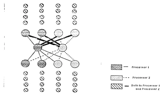
Chapter 5. Parallel [mplementation of Backpropagation Algorithm 19 0 0 0 0 0 © © © © © 0 0 © © 0 © 0 0 © 0 0 0 © m m P r o c e ^ t o r I P r o c e s s o r 2 Do Ift If» P r o c e s s o r I Qful I’ l o c e s s o r 2
Figure 0.1: Mapping backpropagation to multiple processors using Network Partitioning
N etw o rk P a rtitio n in g
In network partitioning, assuming P = 2^ processors available, the units in each hidden layer hidden layer and the output layer are partitioned so that (approximately) the same number of units from each layer are distributed to each processor. This is equivalent to partitioning the weight matrices into horizontal strips and assigning each strip to a processor. For example matrix is partitioned so that the first N/^IP rows are assigned to the first processor, the second Nh!P rows are assigned to the second processor, and so on. The input vector I is available to all the processors. It can be seen that each processor assigned to a portion of the units from each layer needs to have access to the outputs of all the units in the prior layers. For instance, for computing the outputs of the first hidden layer, all the processors need to access all of the input vector I. In a network with a single hidden layer, in order to compute the outputs of the output layer, all the processors need to access all of the output vector H of the hidden layer. Since a given processor computes only a portion of the layer outputs, the processors have to synchronize after each layer computation and then exchange their respective portions of the relevant output vectors by a global communication, so that all the processors get a copy of the output vector for the next stage of the computation (see Figure 5.1). In a network with multiple hidden layers a global communication would be necessary after each hidden layer computation in the forward pass. The total number of global communications performed during the forward pass of the
aigoricum is equal to the number of layers in the network.
The forward pa.ss is completed when each processor computes its portion of 'i'he network output vector O. After the error vector is computed and passed to all the processors, the next step in the backward pa.ss is the computa tion of the error vector for the (last) hidden layer for which the transpose of the weight matrix has to be multiplied with 6^. Since the forward pass requires thcit the weight matrices be distributed to the processors as rows, rnultiplicix- tion with the transpose cannot readily be done. The necessary weight matrix values can be obtained in three different ways.
1. As a first attack to the problem, the weight values necessary at the back ward pass, that are partitioned among the processors can be gathered by a number of communications.
2. The required weight information can be kept at the corresponding pro cessors in addition to the horizontal matrix strips. This requires extra computations to maintain them.
3. Instead of keeping extra information, processors can calculate their par tial 6^ values necessary for the calculation of the overall vector and by a global communication, and a following internal addition can calculate the overall vector.
We select the second approach for the implementation. The first method requires extra communication steps which significantly slows down the algo rithm. The number of communications performed at the third approach is equal to the second one, but the information amount per communication in creases by an amount proportional to log2P. Communication in the hypercube
architecture being a bottleneck, we have opted to do some redundant compu tation instead of communication.
Chapter ö. Parallel [rnplementatinn of Packpropagation Algorithm 2 0
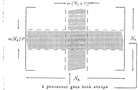
Instead of distributing just the horizontal strips from the weight matrices to the processors, we also distribute a vertical strip as shown by the shaded area in Figure 5.2. During the forward pass, each processor uses the horizontal strip, but during the backward pass it uses the vertical strip for multiplication with the transpose. Thus in the backward pass each processor computes the appropriate portion of locally and then performs a global communication
Chupter 5. Parallel implementation o f Backpropagation .4/<T on>/v •Ti
( -V,. -u n
■No/P No
A processor gets both strips
Figure 5.2; Partitioning the weight matrix for forward and backward passes.
to obtain a copy of the whole 5^ vector for the next stage of computation. The total number of communications performed at the backward pass is equal to the number of layers within the network. If there are more hidden layers, this procedure is repeated. After the computation of the error vectors, each processor computes the weight changes for the portions of the weight matrices assigned to it and then updates the weights in parallel. At this stage some of the computations are redundant since we are essentially keeping two copies of each weight matrix distributed across the processors and we are trading extra storage and redundant computation, for communication.
T ra in in g S e t P a r titio n in g
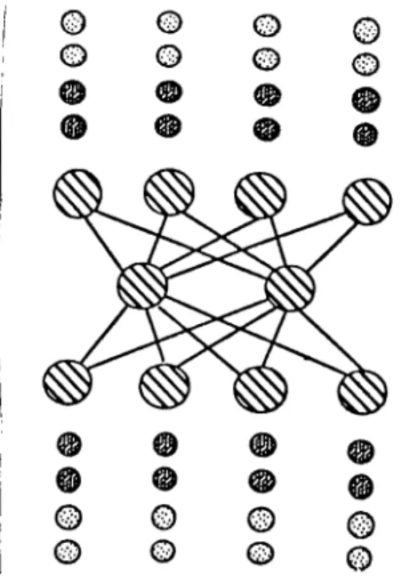
In training set partitioning, the training set of the neural network is par titioned among the processors so that nearly the same number of input output pairs are kept in all processors. In addition to a portion of the training set, each processor keeps a copy of entire network (both units and weights see Fig ure 5.3), and storage for accumulating the total weight change due to its own training set.
In this method, each processor performs the algorithm on its own training set. After all processors have finished calculating weight changes for all their input output pairs, they share their accumulated weight changes with the other
Chapter 5. Parallel Implementation of Backpropagation Algorithm 22 © ©© ©© © P r o c e s s o r 1 P r o c e s s o r 2 B o th In P r o c e s s o r 1 o n d P r o c e s s o r 2
Figure 5.3: Mapping backpropagation to multiple processors using Training Set Partitioning
processors using the communication system. Finally, each processor updates its local weights with the resulting total weight change over whole training set.
In order to parallelize the backpropagation algorithm by partitioning the training set across the processors, it is assumed that the changes to weights due to each input output pattern are independent; that is, the training set can be applied in any order and yield the same result . Clearly, this condition is not satisfied by the on-line version of the algorithm, in which weight changes are calculated and applied after each pattern presentation. Consequently, this kind of parallelism is applicable to only the off-line version of the algorithm.
5.4
O th er P arallel Im p lem en ta tio n s
There have been a number of implementations of backpropagation learning algorithm on a number of different platforms. These include implementation of the NETTalk system on the massively parallel Connection Machine [2], the simulator on the WARP array processor for a neural network for road recog nition and autonomous land vehicle control [16, 17], the implementation of backpropagation on IBM’s experimental G F ll system with 566 processors ca pable of delivering 11 gigaflops [28], an implementation of backpropagation on an array of Transputers [19]. Other massively parallel systolic VLSI emulators for artificial neural networks have also been proposed [18, 11].
I he ('onnerf.ion n, highly p?,r:'!!o! '^omputs-r 'j'yiiiigar.Lblc .vuli
bctvvcc;!! iG,3o4 lo o5,o3o processors. The implementation of NetT->lk system on a Comicctioa Machine with lo К prore'^sors otters a speed up of 500 O'v'cr a similar iinpleinentation of the backpropagation algorithm on V AX -11/780, and a speed up of 2 over an implementation on Cray 2 [2].
The WARP machine is a programmable systolic array composed of a linear array of 1 0 processors. Each processor is capable of performing a peak rate of
10 million floating point operations per second. The backpropagation simulator implemented on WARP machine is first implemented using the second type of parallelism (see Section 5.1) , then it is implemented using the third type of parallelism. It is experimented that second implementation of the algorithm performs much better than the first implementation. It is reported that the second implementation can update 17 million weights per second, and this is 6
to 7 times faster than a similar simulation running on Connection Machine [17].
The G F ll is an experimental SIMD machine consisting of 566 processors. Each processor is capable of performing 20 million floating point operations per second. The implementation of backpropagation simulator for G F ll Sys tem is planned to be used for continuous speech recognition. The simulator implemented for G F ll which uses the third type of parallelism approach, is estimated to deliver 50 to 100 times the performance of the WARP implemen tation [28].
Chapter 6
H Y P E R B P - The Parallel Backpropagation
Simulator
The ilYPERBP tool is a library of C functions for the iPSC/2 hypercube mul ticomputer system. Using these functions in an appropriate order, a user can create a backpropagation neural network, train it with the standard backprop agation learning algorithm, simulate it, and obtain the simulation results.
A user who wants to use the simulator HYPERBP has to write a C program and has to include the definition file namely common.h at the top of his pro gram. This file includes necessary type definitions and constant declarations. The user must also include a header file depending on the parallel version to be used. If the user wants to use the training set partitioning method then trainset-part.h header file is to be included at the top of the program. If the network partitioning method is to be used then the network.part.h header file must be included. The user also has to write a block called Backpropagation Block in the program. This block consists of a set of C statements and calls to the simulator functions.
Backpropagation Simulation and Training Tool functions can be classified into seven categories:
1. Backpropagation Block Delimiter calls, 2. Neural Network Definition calls,
3. Training Parameter Setting calls.
4. I r a i a i n g .'Det, ,'i[)ecitu:a.tion ra ils ,
5. Neural Network Simulation calls, 6. Neural Network Training call, and 7. Information Retrieval calls.
6.1
B ackpropagation B lock D elim iter Calls
The backpropagation block begins by a bp^begin call and ends by a bp-end call.
bp_begin
The function call bp-begin marks the beginning of the backpropagation sim ulation block within the C code. It is the first function to be called in the backpropagation block. The function has the following form :
('I];ipter o’. f l YFKI l Bl · ’- /■ 'araii'·.'/ ii.ic.':p;'opa,:^'a:;Ga Si^iUilaLui· 2o
INTEGER} bp-begin(n.of-prcs, name-of-cube) INTEGER Ji-of-prcs;
char *name-of-cube;
The bp-begin call takes two parameters. The first parameter, n-of.prcs,
specifies the number of processors to be used during training , and simulation. The second parameter, namc-of-cube^ is the name to be given to the allocated cube.
After the execution of this call, a hypercube named namc-of-cube, con sisting of possibly n-of-prcs is allocated; the number of processors successfully allocated is returned as a result.
The number of processors allocated for a process has to be a power of 2. This is due to the requirements of the iPSC/2 hypercube multicomputer system (see page 17). Thus, if the value of parameter, n.of-prcs is not a power of two, this value is rounded to the next power of two, and then a cube consisting of
Chapter 6. HYPERBP - The Parallel Backpropagation Simulator 26
that many number of processors is allocated. Example :
A user can do a simulation with a cube named deniz with 4 pro cessors, by the following call.
k=bp-begin(4, “deniz”);
If the number of processors available at that moment is 4 or greater, then the function will allocate a cube named ’’deniz” with 4 processors. Under such circumstances the value of variable k will be 4. But, if the number of processors available in the s3^stem at that moment is less than 4, then the largest possible cube will be allocated, and its number of processors will be returned as a result of the call.
bp_end
The function call bp.end marks the end of the backpropagation simulation block within the C code. It is the last function called at the end of backpropagation block. The function has the following form :
void bp-end()
6.2
N eu ral N etw ork D efin itio n Calls
In the backpropagation block, first the neural network to be used is declared. This declaration is surrounded by the bp-def-begin and bp.def-end calls.
bp_def_begin
The function call bp-def-begin marks the beginning of the neural nctv.'ork dec laration within the backpropagation block. The function has the following form:
INTEGER bp-def.begin (n-ofJnyerfi) INTEGER n.ofJayers;
('haptf'r в. H Y P E R B P - The Parallel Backpropa^atlon Simiihitor 2 7
The hp-defJyegin rail takes one parameter. 'The parameter, n.of Jayers spec ifies the luaiiber of layers in the network. This is hiddenlayer[s)-\-onfpntlnyer.
After the execution of this call, the value of the parameter n-oJJayers is returned if such a number of layers is acceptable, otherwise 0 is returned otherwise.
b p -in p u t
The function bp-input defines the input layer of the network. It has the follow ing form :
INTEGER bp-input (n-of-nodes, bias.flag) INTEGER n-of-nodes;
BOOLEAN^ bias-flag;
The bp-input call takes two parameters. The first parameter, n-of.nodes specifies the number of nodes to be used in the first layer, namely the input layer of the neural network. The second parameter, bias-flag speciRes the existence of a dynamic biasing node in the input layer. If the bias-flag has a TRUE value, then an extra special node is augmented to the input layer. The activation value of this node is always one. Its weights on the connections to the upper layers are automatically updated like other ordinary nodes during training. These weights are used as a dynamic biasing factor during the calculation of the activation values in the upper layer.
After the execution of this call, the value of parameter n-of-nodes is re turned, if there is no error, otherwise a 0 is returned.
b p _ h id d en
The function bp.hidden defines a hidden layer of the network. It has the fol lowing form :
Chr'tpt.er 6. H Y P E R B P - The Parallel Back propagation SlniuldLor 2S
ii'iTEGER ¡)[)Jiiddta(hl-index, n..of.nodes, afptr, epfpir, hias-jlaq) INTEGER hLindcx; INTEGER n-of.nodes; ADDTYPE afptr; ADDTYPE epfptr; BOOLEAN biasGlo,g;
The bp-hidden call takes five parameters. The first parameter, hLindex specifies the hidden layer being defined, since, a neural network may have more than one hidden layer. All these layers must be defined one by one using the successive bp-hidden calls. The hLindex parameter distinguishes hidden layers, the hidden layer following the input layer has an index 1, while the hidden layer following it has an index 2, etc. The second parameter, hLindex specifies the number of nodes at the hlJndex*^ layer. The third parameter, afptr is a function pointer to a library function, which will be used for calculating the current hidden layer nodes activation values. When a NIL value is passed as the pointer value, the default C function is used to calculate the activation value. The default function is the standard sigmoid function. The fourth parameter, epfptr is a function pointer to a C function, which will be used for propagating the error values of the current hidden layer. When a NIL value is passed as the pointer value, the default C function is used as the error propagation function. The last parameter, bias.flag is a biasing flag parameter similar to the one in the bpJnput function.
After the execution of this call, the value of parameter n-of-nodes is re turned if there is no error. Otherwise a value of 0 is returned.
b p -o u tp u t
The function bp-output defines the output layer of the network. It has the following form ;
Chapter 6. H Y P E R B P - T h e Parallel Da.ckpropaga.tlon Sinmhitor 2 9
INTEtrEfi n-of-Tiode.'^;
-ADDTYPE afptr;
The bp-hidden call takes two parameters. The first parameter, n.of-iiodes specifies number of nodes in the output layer of the neural network. The second parameter, afptr is a pointer to a function, which will be used to calculate the activation values of the nodes in the output layer. When a NIL value is passed as the pointer value, the default C function is used to calculate activation value. The default function is the standard sigmoid function.
After the execution of this call, the value of parameter n^of-nodes is re turned if there is no error. Otherwise a value of 0 is returned.
bp_def_end
bp-def-end marks the end of the neural network declaration within the back- propagation block. The function has the following form :
void bp-def-end()
After this call, a neural network with the specified properties is built. Ex a m p l e:
A user can define a neural network with 3 layers, by the following function calls.
bp-def-begin(3);
bp-input(6, TRUE);
bp-hidden(l, 10, NIL, NIL, TRUE); bp.hidden(2, 3, NIL, NIL, TRUE); bp-output(4, NIL);
bp-def-end();
There are 4 input nodes and an extra biasing node. The first hidden layer will have 10 nodes, and an extra biasing node. The default ac tivation function will be used for these nodes, also at the backward
Chixptcr 6. I[\'P E IIB P - I he PiimUel BiickpL^opclgгítion Simulator 3 0
pass of the learning algorithm default error propagation functions will be used. The second hidden laver will have 3 nodes, and an extra biasing node. Also the default functions will be used for the nodes in this layer. The output layer will consist of 4 nodes, and these nodes will use the default activation function.
6.3
Training P aram eters S ettin g Calls
The parameters to be used during the learning process are momentum, learning rate, and the initialization range. These parameters are set using the following calls.
b p _ se tm o m en tu m
The function call bpsetmomentum sets the value of the momentum term to be used in the backpropagation learning algorithm.
void hp-setmomentum (momentum-value) SIMTYPEP momentum-value;
The function has only one parameter. The value of parameter momen tum-value is used to set the momentum term of the learning algorithm. If this function is not called within the backpropagation block, the default momentum value of 0.9 is used.
b p -s e tle a r n in g r a te
The function call bpsetlearningrate sets the value of the learning rate term to be used in the backpropagation learning algorithm.
void bp-setlearningrate(learning-rate-value) SIM TYPE learning-rate-value;
^The type SIMTYPE symbolizes the type of the simulation going on, this value can be long or float.
Chapter 6. H Y P E R B P - The Parallel Backpropagation Simulator 31
TIxc fuucLiua has only one parameter. I he parameter, learning.rate .value's is used to set the learning ra.te term of the learning algorithm. If this function is not called within the backpropagatioii block the default learning rate value of 0 . 2 is used.
bp _ ran d o m ran g e
The function call bp.randomrange sets the upper and lower limit values to be used during weight matrix initializations, with random numbers. This weight randomization process is actually the first step of the backpropagation learning algorithm.
void bp-randomrange(lower, upper) SIM TYPE lower, upper;
The function has two parameters. The first parameter, lower, is used as the lower limit, and the second parameter, upper, is used as the upper limit value during the random initialization. If this function is not called within the backpropagation block the default limits, 0 and 0.32767 are used.
6.4
T raining S et S pecification Calls
The training set of a neural network problem can be introduced to the simula tion and training tool in two steps. First, the input pattern set is introduced by bp-setinput or bp..setsinput call, and then the target pattern set is introduced by the calls bpsettarget or bpsetstarget.
b p _ se tin p u t
The function bpsetinput defines the input patterns of the training set. The function has the following form :
Chapter 6. H Y P E R B P - The Parallel Backpropagation Simulator 3 2
SIM TYPE '■ ‘"b.add-in put;
ii\'TEGER a .of.pattern
The bp.setinput ca\{ takes two parameters. The first parameter, h .add.input, is a pointer to a matrix containing the input patterns of the training set. One input pattern resides in each row of the matrix. The number of columns of this matrix must be equal to the number of nodes at the input layer. The second parameter, n.of-patterns specifies the number of input patterns that is being defined. Thus, it specifies the training set size of the neural network. This call returns the value of n-of-patterns parameter if there is no error. Otherwise, it returns a value of 0.
b p _ se tta rg et
The function call bpsettarget introduces the target (in other words, destina tion) patterns of the training set. The function has the following form :
INTEGER bp.settarget(b-add-target,n.of.patterns) SIM TYPE **b-add-target;
INTEGER n-of.patterns;
The bp.settarget call takes two parameters. The first parameter, b.add.target, is a pointer to a matrix containing the target patterns of the training set. One target pattern resides in each row of the matrix. The number of columns of this matrix must be equal to the number of nodes at the output layer. The second parameter, n-of.patterns, specifies the number of target patterns that is being defined. Thus, it specifies the training set size of the neural network. This value has to be consistent with the number of input patterns specified in the calls bp.setinput or bp-setsinput.
This call returns the value of n-of.patterns parameter if there is no error. Otherwise, it returns 0.
The training set of many neural network problems requires sparse input patterns and/or sparse target patterns. These sparse patterns consists of lot
of 0 <.Liiu voiy few 1 Vcilues. In order to introduce such patterns in
an efficient way two special functions arc implemented in IIYPERDP; called, bp.setsinput and bpsetstarget.
While preparing the pattern array for the calls bpsetsinput and bp^setstarget the user has to place one pattern at each row of the array in a coded way. In each row there are n + 1 elements, where n is the number of 1 values within that pattern. The first element of the row holds the value n. The following n elements of the row specify the indices of the input unit to which the value I has to be applied.
b p _ setsin p u t
The function bpsetsinput introduces the sparse input patterns of the training set. The function has the following form :
INTEGER bp-setsinput(b-add.input,n.of.patter ns) unsigned char **b-add-sinput;
INTEGER n-of-patterns;
The bp-setsinput call takes two parameters. The first parameter, b.add.sinput, is a pointer to a matrix containing the input patterns of the training set in a coded form as explained above. One input pattern resides in each row of the matrix. The second parameter, n-of-patterns, specifies the number of input patterns that is being defined. Thus, it specifies the training set size of the neural network.
This call returns, the value of n-of-patterns parameter if there is no error. Otherwise, it returns 0.
In a backpropagation block there can be a bpsetinput or hp.setsinput call, but not both.
b p _ se tsta r g e t
Ciuxpter 6. H Y P E IiB P - llw P;)ralP'l Barkpvopagation SirmiUitoi· 33
Chapter 6. H Y F E ltB P - The Parallel Back-propagation Simulator 3 4
INTEGER i)p-:ietstarget(b.add-starget,nmf.patterns) unsigned char “h aild starget;
INTEGER n.of.paLtenis;
The bpsetstargetcall takes two parameters. The first parameter, b-add-target, is a pointer to a matrix containing the target patterns of the training set in a coded form as explained at page 33. One target pattern resides in each row of the rnatri.x. The second parameter, n..of.patterns, specifies the number of target patterns that is being defined. Thus, it specifies the training set size of the neural network. This value has to be consistent with the number of input patterns specified in the calls bpsetinput or bpselsinput.
This call returns the value of n-of-palterns parameter if there is no error. Otherwise, it returns a value of 0.
In a backpropagation block there can be a bp..settarget or bp^setstarget call but not both.
6.5
N eu ra l N etw ork Sim ulation Calls
The functions bp.forward and bpsforward perform a forward pass over the defined neural network with the given input pattern.
v o id bp_forw ard
bp-forward simulates the current neural network. It actually performs a forward pass of the backpropagation learning algorithm with the specified input vector. The function has the following form :
void bp-forwardfan-input-pattern) AD D TYPE an-inpuLpattern;
The function bp-forward takes only one parameter. The parameter, an-inpuLpattern is a pointer to an input vector. This input vector is applied to the input layer
C h a p t e r 6\ II Y P E R B F - The P¿ır¿iItel Backpropa^^ation Simulator .So
void bp-sforw ard
The hp sfonrard simulates the current neural network. It ¿ictually perluriiis a forward pass of the backpropagation learning algorithm, with the specified sparse input vector. The function has the following form :
void bp-sforwardfan^sinput-pattern) unsigned char anAnput^pattern;
The function bp-sforward takes only one parameter. The parameter, a n . s i n p i L t . p a t t e r n
is a pointer to an input vector which is coded as explained at page 33. This input vector is forwcirded to the input layer and a forward pass is performed over the neural network.
6.6
N eu ral N etw ork Training Call
The function call bpJearn performs the forward and backward passes of the backpropagation learning algorithm.
b p -lea rn
bpJearn performs a specified number of epochs of the backpropagation algorithm to the defined network.
long bpJearn(n-of-patterns, n-of.epochs, online-flag) INTEGER n-of-patterns, n-of-epochs;
BOOLEAN online-flag;
The function takes two parameters. The first parameter, n-oflepochs, spec ifies the number of epochs to be performed. The second parameter, online-flag, specifies the version of the program to be used. If this parameter has the value TRUE then the on-line version of the algorithm is performed. Otherwise, the off-line version of the algorithm is performed. But note that, with training set