Superior Performance of Switched Fuzzy Control Systems: an Overview and
Simulation Experiments
Vesna M. Ojleska and Tatjana
Kolemishevska-Gugulovska
Faculty of Electrical Engineering and Information Technologies (FEEIT)
SS Cyril and Methodius University Skopje, Republic of Macedonia e-mail: {vojleska, tanjakg}@feit.ukim.edu.mk
Georgi M. Dimirovski
School of Engineering Dogus University
Istanbul, TR-34722, Republic of Turkey FEEIT, SS Cyril and Methodius University
Skopje, Republic of Macedonia [email protected]
Abstract —This article gives a brief overview of the basic notions of switched fuzzy systems, their model construction and stability analysis, followed by the proposed concepts for building simulation algorithms for this type of systems. Using these concepts we have shown the whole process of modelling, stability analysis and design of stabilizing switching fuzzy logic controllers for the hovercraft-vehicle as a typical nonholonomic system. MATLAB Simulator (Simulink model) and special MATLAB functions for the switching fuzzy controller of the hovercraft vehicle, along with the numerous simulation results, verify the correctness of the proposed concepts. Using this typical nonholonomic system we have also explored the good performance of switched fuzzy systems in comparison to the ordinary T-S fuzzy systems.
Keywords –control, hybrid systems, fuzzy systems, switched systems, switching, simulation of switched fuzzy systems
I. INTRODUCTION
Switched systems are special class of hybrid dynamical systems, which consist of a set of continuous-time or discrete-time subsystems and a rule that coordinates the switching among them. The last couple of decades have witnessed an enormous growth of interest of the class of switched systems in combination with the even larger class of hybrid systems [1], [2], [3], [4], as these systems have a wide range of potential applications.
From the middle of the 1980’s, there have appeared a number of analysis/synthesis problems for Takagi-Sugeno (T-S) fuzzy systems [5], [6], [7].
Succeeding the remarkable developments in theory, applications, and the industrial implementations of fuzzy control systems, recently switched systems have been extended further to encompass switched fuzzy systems [8].
In general, a switched fuzzy system involves fuzzy systems among its sub-systems or an alternative fuzzy-switching law, or the both (least explored case). Resent developments in this area promote a new direction in the control of dynamic systems [9], [10], [11], [12], [13], [14], [15], [16], [17], [18], [19] and it is clear that the field of switched fuzzy systems is becoming very popular.
To our best knowledge, it may well be found that up to know the most of the research in this area is focused on representation modelling, stability analysis and controller design, that guarantees stabilization and certain system performance. We are expecting that these results can be used as a good platform for solving real world control problems. Thus, in this paper we are proposing the simulation scheme algorithms that can be used in modelling and design of
switching fuzzy controllers for real world systems and we continue with exploring the performance of switched fuzzy control systems. The model of a hovercraft vehicle (a typical nonholonomic system that can not be stabilized by any continuous feedback control law) is used to verify the proposed simulation schemes as well as to prove the good performance of switched fuzzy systems.
Since in [20] and [21] we have given a detailed overview of the achievements in the field of switched fuzzy systems, followed by the comparative study for this kind of systems (different approaches in their model construction and challenges associated with the stability analysis and stabilization), here, we have provided a discussion of some of the key principles of the joint concept. This paper is an extension of the study given in [22].
To begin with, in Section II we give a brief overview of the basic concepts of switched fuzzy systems and their representation modelling. Appropriate stability analyses for this type of systems are given in Section III. In Section IV we outline the proposed concept for building simulation algorithms for switched fuzzy systems. In Section V the dynamics of a hovercraft vehicle as a typical nonholonomic system is given. For the purpose of later comparison, in Section VI we have given the whole process for building normal (non-switched) T-S fuzzy controller for the hovercraft vehicle, showing that with this type of controllers the control purpose can not be achieved. Using the proposed simulation schemes from Section IV, in Section VII we present the whole process of modelling and design of the switching fuzzy controllers for the hovercraft vehicle. We conclude this section with numerous simulation results, proving the good
performance of switched fuzzy control systems. In Section VIII we give the essential conclusions of this study.
II. CONCEPTS OF SWITCHED FUZZY SYSTEMS AND REPRESENTATION MODELLING
The idea for switched fuzzy systems was putted forward by Palm and Driankov in 1998 [8]. Tanaka et.al. according to their previous research in the field of T-S fuzzy systems, for the purpose of control of more complicated real systems such as multiple nonlinear systems, switched nonlinear hybrid systems, and second order nonholonomic systems, introduced new type of model-based fuzzy systems - switched fuzzy systems [9]-[11]. The main aim of this design approach was to lose the “curse of dimensionality” - the complexity of a system makes the number of rules of a fuzzy model exponentially increase. Differently from the ordinary T-S fuzzy model, the switching fuzzy model given in [9]-[11] has locally Takagi-Sugeno fuzzy models (local fuzzy rule level) and switches them according to the premise variables, i.e., states, measurable external variables and/or time (region rule level). In general, the switching fuzzy model has two key features. One is to switch local T-S fuzzy models represented in each region. The other is to decrease the number of rules which fire simultaneously in comparison with an ordinary fuzzy model. Moreover in [9] a stable fuzzy switching control design is presented, where the design conditions are based on “common” quadratic Lyapunov function (CQLF), expressed in linear matrix inequality (LMIs - [7], [24]) form. The same idea is extended further in [10] where the switching controller is constructed by naturally extending the idea of the parallel distributed compensation (PDC) [7], [25].
Parallel to these results, authors in [15] propose T-S fuzzy model which differs from existing ones in the literature and is based on the fuzzy controller switching. Switching PDC controller is designed for a linear fuzzy system based on the switched systems model, i.e. every sub-controller is a PDC controller. Continuous way and discrete way are adopted to establish the stability results. First, sufficient conditions for asymptotic stability are presented and then, stabilizing switching laws of the state-dependent form are designed. Different from [15], where the controller switching strategy is employed to the ordinary T-S fuzzy model, authors in [16]-[18] propose switched fuzzy model for continuous ([16], [17]) and discrete case ([16]-[18]). The switched fuzzy model is seemingly similar to the model proposed in [9]-[11], but there is a crucial difference (the details for these, along with the detailed comparative study for these two approaches, are given in [21]).
Even though there many different approaches on representation modelling of switched fuzzy systems, the typical design procedure, which is present in most of the works, consists of the following steps. First, the whole state-space n
R is partitioned on m regions, and every region is a switched sub system. While functioning, this is the level where via the appropriate switching law an appropriate sub system is chosen to be on. The sub system on every region
i
is represented by a suitable model. When the subsystems of the switched system are represented as T-S fuzzy systems
the system is switched fuzzy system. T-S fuzzy system partitions the space in the corresponding region into fuzzy sub-regions. In that way, the whole state-space is partitioned into many fuzzy sub-regions, where every sub-region is represented by a local model. The local model can be linear or nonlinear, continuous time or discrete time.
Figure 1. Sketch map of switched fuzzy system [19].
The sketch map of switched fuzzy system, regarding the state-space partitioning, is depicted on Fig. 1. In there, i
denotes the state-space area of the i-th switched subsystem. il
denotes the l-th fuzzy sub-region in the region i. In
fact, the switched fuzzy systems partition the i region into
l fuzzy sub-regions i1,,il,,i . There is a local
linear/nonlinear model in every fuzzy sub-region. The model for every switched region 1,,m, which consists of local
linear/nonlinear models, is composed by linking the local models with fuzzy membership functions. When local model in fuzzy sub-region satisfies the switching law, switching to the i-th subsystem is made. In this way, stability of the switched fuzzy system, as a whole, is ensured.
For better understanding the concept of switched fuzzy systems, we will proceed by presenting one of the two basic analytical representations, analysed in [21], the so-called “switched fuzzy system with levels of structure”, given in [9]-[12]. The purpose for choosing this type of representation modelling is that the analysis given in this paper is based on this type of modelling.
The model in [9]-[12] has local T-S fuzzy models and switches them according to the premise variables, i.e., states, measurable external variables and/or time. The switched fuzzy model from [9]-[12] is given with:
l r i m t x C t y t u B t x A t x M t z M t z l N t z N t z i il il il ilp p il ip p i , , 2 , 1 , , 2 , 1 , , , : , : 1 1 1 1 THEN is and and is IF Rule Plant Local THEN is and and is IF Rule Region (1)In (1), m is the number of regions partitioned on the
of rules of the local models; Milj is fuzzy set; x
t Rn is thestate vector,
m R tu is the input vector, y
t Rq is theoutput vector, nn il R A , Bil Rnm , and qn il R C ;
t
z
t z
t
z 1 ,, p are known premise variables that can be
functions of the state variables, external disturbances, and/or time. Nij
z
t is a crisp set, where:
w o N t z t z Nij 0 , . ij , 1 . (2)From (1), it is clear that the switched fuzzy model has two levels of structure: region rule level and local fuzzy rule level. The region rule is crisply switched according to the premise variables. In other words, the membership functions Nij
z
tin the premise parts of the region rules are crisp sets.
The switched fuzzy model (1) is inferred by fuzzily blending the linear system models x
t Ailx
t Bilu
t andswitching the global T-S fuzzy models, defined on every region.
Given a pair of
x ,
t ut
and z
t , the final output of thefuzzy system is inferred as follows:
m i r l il il il izt h zt A xt B ut t x 1 1 (3)
m i r l il il izt h zt C xt t y 1 1 (4) where
m i p j j ij p j j ij i t z N t z N t z 1 1 1 ,
r l p j j ilj p j j ilj il t z M t z M t z h 1 1 1 (5)It is clear from (2) and (5) that
. . , 0 , 1 w o i t z t z i Region . This means that i
z
t 1 ifand only if z
t belongs to “Region i ”. The regions satisfy:
m i i m 1 21 Region Region Region
Region (6) m i m i i i i i1Region 2,1 2, 11,, , 21,, Region , where
denotes the universe of discourse.
In [9], authors propose a new PDC to design a stable switching fuzzy controller for the switched fuzzy system (1). The idea for designing a PDC controller is a natural extension of the same concept, used for the ordinary T-S fuzzy systems (see for example [7]).
t Fx
t l r i m u M t z M t z l N t z N t z i il ilp p il ip p i , , 2 , 1 , , 2 , 1 , , : , : 1 1 1 1 THEN is and and is IF Rule Control Local THEN is and and is IF Rule Region (7)Finally, the overall fuzzy controller is represented by:
m i r l il il izt h zt Fxt t u 1 1 (8)By substituting (8) into (3), the fuzzy control system can be represented as:
m k r i r j kj ki ki kj ki k m k m l r i r j lj ki ki lj ki l k t x F B A t z h t z h t z t x F B A t z h t z h t z t z t x 1 1 1 1 1 1 1 (9)III. STABILITY ANALYSIS AND CONTROL DESIGN
Compared with the results on stability of switched systems and those of T-S fuzzy systems, the results on switched fuzzy systems are very few. Similar to the stability analysis for model based T-S fuzzy systems ([7]) and switched systems ([1]-[3]) alone, stability analysis of switched fuzzy systems has been pursued mainly based on Lyapunov stability theory but with different Lyapunov functions. One of them is the so-called common (or global) quadratic Lyapunov functions, another one is the so-called
piecewise quadratic Lyapunov functions, and the third one is
the so-called fuzzy (or non-quadratic) Lyapunov functions. Regardless of the different Lyapunov functions that are used, the typical design procedure, common for most of the papers, concerning switched fuzzy systems, includes the following:
Stability analysis and derivation of asymptotic stability conditions for autonomous system;
Synthesis of the parameters of the predefined controllers that will stabilize the system [9]-[14], as well as (or) derivation of stabilizing switching laws (signals) that will stabilize the system [15]-[19]. As in Section II we outlined one of the two typical approaches for representation modelling of switched fuzzy systems, here we will summarise the conditions for
asymptotic stability for this kinds of models, as well as the conditions for designing controllers for stabilizing this kind of systems. Detailed analyses on the stability results of switched fuzzy systems, based on the different types of Lyapunov functions, are given in [21].
Considering the literature related to T-S fuzzy model based systems ([5], [7]) it can be well found that the Linear Matrix Inequalities (LMIs - [7], [24]) play an important role in stability analysis of this kind of systems. Very natural, authors in [9]-[12], extend their previous works, considering stability of ordinary T-S fuzzy systems (expressed in the form of LMIs - see [7]), in the field of switched fuzzy systems. Bellow, we will address the stability conditions for the open-loop system (model (1)), as well as the stability and relaxed stability conditions for the closed-loop system (model (9)), given in [9]-[12].
A. Stability Conditions of Switched Fuzzy Model with Levels of Structure
To begin with, we show a stability condition (based on quadratic Lyapunov function (10)) for the switched fuzzy system (1), when u0.
xt x
t PxtV T , 0P . (10)
Note that Theorem 1 is taken from [13] and [14], although it addresses the stability problem given in [12].
Theorem 1 [12] ([13] and [14]): The switched fuzzy
system (1), for u0, is asymptotic stable if there exist a positive definite matrix P , satisfying the following LMI conditions: 0 il T ilP PA A , l,i. (11)
The condition (11) is easily derived by taking the time derivative of equation (10) along the trajectories of the system (1).
B. Stable Controller Design of Switched Fuzzy Model with Levels of Structure
Here we will focus on the LMI stability conditions as well as LMI relaxed stability conditions for the closed-loop system (9) - system that consists of the switched fuzzy model (1) and the appropriate PDC controller, given with (7). The LMI stability conditions are obtained with respect to P1
X and
X F
Mil il (note that these LMI conditions correspond to the
LMI (relaxed) stability conditions for the ordinary T-S fuzzy model-based systems given in [7]). The PDC fuzzy controller design is to determine the local feedback gains F in the il
consequent parts. As it is mentioned in [7] and [9], although the PDC fuzzy controller (8) is constructed using the local design sense, the feedback gains F should be determined il
using the global design sense (stability conditions for the global stabilization of the system).
Theorem 2 [9], [10] (stability): The switched fuzzy model
(3) can be stabilized via the PDC switching fuzzy controller
(8), if there exist a common positive definite matrix X , such that: 0 il il T il T il il T il A X M B B M XA , (12) for i1 ,2, ,m, l1 ,2, ,r and 0 il ik T ik T il ik il T il T ik ik T ik il T il M B B M M B B M X A XA X A XA (13)
for all i and lk excepting all the pairs
l,k such that
zt h
z
t 0 hil ik , t, where 0 1 P X , Mil FilX.Proof: See [9] and [10].
According to Theorem 2, stability analysis of the switched fuzzy control system is reduced to a problem of finding a common P. If r, that is the number of IF-THEN rules, is large, it might be difficult to find a common P satisfying the conditions of Theorem 2. In Theorem 3, these conditions are relaxed.
Theorem 3 [9], [10] (relaxed stability): Assume that the
number of rules that fire for all t is less than or equal to , where 1 r . The switched fuzzy model (3) can be
stabilized via the switching PDC fuzzy controller (8), if there exist a common positive definite matrix X and a common positive semi-definite matrix Y , such that: i
1
0 T il il i il T il il T il A X M B B M Y XA , (14) for i1 ,2, ,m, l1 ,2, ,r and 0 2 il ik T ik T il ik il T il T ik ik T ik il T il i M B B M M B B M X A XA X A XA Y , (15)for all i and l excepting all the pairs k
l,k such that
zt h
z
t 0 hil ik , t and m1, where 0 1 P X , X F Mil il , 0Yi XQiX .Proof: see [9], [10] and [12].
Except stability (relaxed stability) theorems for the switched fuzzy system (1), authors in [9]-[12] also present the conditions for the constraints on control inputs. These conditions match the corresponding ones for ordinary T-S fuzzy systems, given in [7].
Consider each input variable, i.e. [9]-[12]:
m i r l il il i k k k t Eut E zt h zt F xt u 1 1 (16) where Ek
k
f 1 0 1 0 .Theorem 4 [11], [12] (constraints on the control inputs):
constraint uk
t 2k (k1 ,2, ,f) is enforced at all timesif the following LMIs hold:
0 0 0 1 X x xT , 0 2 I M E E M X k il k k T il , l , i , k , (17) where 10 PX and Mil FilX are LMI variables.
Proof: See [12].
IV. PROPOSED SIMULATION ALGORITHMS
In this section we will present the proposed concepts for building simulation algorithms for switched fuzzy control systems which is the main contribution of the presented work.
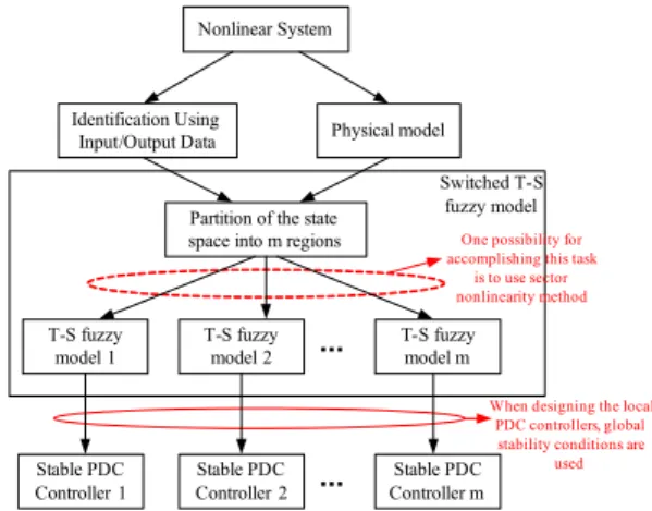
First, we present the whole process for designing the switching fuzzy controller for the given nonlinear system. This is given on Fig. 2. As it is obvious from Fig. 2, first we have to find the switched fuzzy model for the nonlinear system, after what (using certain conditions) we will synthesize the appropriate switching PDC controllers. The final aim is to generate stable controllers which will satisfy certain stability conditions given in a form of LMIs (e.g. using Theorem 2 or Theorem 3).
...
...
Nonlinear System
Identification Using
Input/Output Data Physical model
Partition of the state space into m regions
T-S fuzzy model 1 T-S fuzzy model 2 T-S fuzzy model m Switched T-S fuzzy model
One possibility for accomplishing this task
is to use sector nonlinearity method Stable PDC Controller 2 Stable PDC Controller 1 Stable PDC Controller m
When designing the local PDC controllers, global stability conditions are
used
Figure 2. Switching fuzzy controllers design.
Next, we propose one possible way for finding this stable switching fuzzy logic PDC controllers (using MATLAB), after what, with the appropriate Simulink model, we can make the performance analyses simulations. The necessary steps are represented on Fig. 3. After the local switching controllers are generated (using the algorithm on Fig. 3), according and for the appropriate switched T-S fuzzy model (Fig. 2), they can be used for controlling the real nonlinear system. Choosing the appropriate controller in certain moment (switching among these controllers) is made according the conditions which define the certain region selection. This is shown on Fig. 4. In every region there is an appropriate stable PDC controller which is synthesized using the design procedure given on Fig. 3.
Parameters that define the linear systems in every region, initial conditions and design constraints
LMI Design (“Robust Control Toolbox” -MATLAB) Design of T-S PDC controllers Simulink model Performances Fil
Figure 3. Steps for controller design and performance evaluation for the given switched fuzzy model.
Region 1 Region 2 Region m Real System Switch Region selection according the predefined conditions ... u x
Figure 4. Control of a real system with previously designed controllers, according the procedure given on Fig. 3.
V. HOVERCRAFT VEHICLE (HV) AS A TYPICAL
NONHOLONOMIC SYSTEMS
A hovercraft is a craft capable of travelling over surfaces while supported by a cushion of slow moving, high-pressure air which is ejected against the surface below and contained within a "skirt".
Figure 5. The model of a hovercraft vehicle [9].
From Fig. 5 it is obvious that if we apply the same force to both motors, the vehicle will go straight, and if different force is applied, the vehicle will turn.
According to hovercraft model of Fig. 5, the following state-space model of the hovercraft vehicle is given in [9]:
t f t M t y t x1 1sin 1 , x2
t yt x1
t
f
t I l t t x3 sin 2 , x4
t t x3
t (18)where f1
t fR
t fL
t , f2
t fR
t fL
t , is the angleof the vehicle; l is the distance between the gravity and fans;
is the angle between the gravity and fans; fR and fL are
the forces generated by the right and left side fans, respectively; M and I are the mass and the inertia,
respectively. The control purpose is lim
0 yt t and
0 lim t t , by manipulating fR
t and fL
t .Using the theory for nonholonomic systems in [1], it can be easily shown that the hovercraft vehicle, with the model (18), is a typical nonholonomic system. Nonholonomy means that the system is subject to constraints involving both, the position and velocity, whereupon it is shown that this systems can not be stabilized by any continuous feedback law [1].
Moreover, for proving this conclusion we will try to stabilize the system with the continuous control law (based on the T-S fazzy model), and then we will design a switching controller, based on the switched fuzzy-logic model.
VI. T-S FUZZY MODEL BASED CONTROL FOR THE HV A. T-S Fuzzy Model for the Hovercraft Vehicle
The design of T-S fuzzy model for the hovercraft system will be made according to the presented design procedure for building T-S fuzzy models in [7].
The main feature of the T-S fuzzy model given in [7] (equation 2.1 – Chapter 2) is to express the join dynamics of each fuzzy implication (rule) by a linear system model.
We replace the equations (18) with an ordinary T-S fuzzy model. The idea of sector nonlinearity is employed in the T-S fuzzy model construction ([7] - Chapter 2).
To begin with, we replace sin
t with a fuzzy modelrepresentation. By considering that
t
, the range of sin
t is given with sin
t
1 1
(this isvisible from Fig. 6-a):
a) b)
Figure 6. a) Nonlinearity sin
t , for
t
; b) Membership functions v1
and v2
.Subsequently, the nonlinear function sin
t can beconverted into the following fuzzy model representation:
2 1 sin i i i t b v t , (19) where
2
1 1 t v t v . (20)From (19) and (20) the membership functions v1
t and
tv2 are calculated as:
2 sin 1 1 t t v ,
2 sin 1 2 t t v , (21)and they are plotted on Fig. 6-b.
We construct the following fuzzy model by utilizing the representation (19) and the membership functions (21).
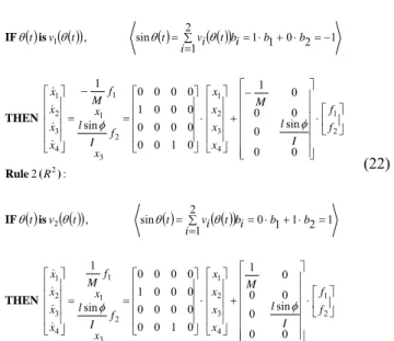
2 1 4 3 2 1 3 2 1 1 4 3 2 1 2 2 2 1 4 3 2 1 3 2 1 1 4 3 2 1 1 1 0 0 sin 0 0 0 0 1 0 1 0 0 0 0 0 0 0 0 0 1 0 0 0 0 sin 1 1 2 1 1 0 2 1 sin , : 2 0 0 sin 0 0 0 0 1 0 1 0 0 0 0 0 0 0 0 0 1 0 0 0 0 sin 1 1 2 0 1 1 2 1 sin , : 1 f f I l M x x x x x f I l x f M x x x x b b i vi t bi t t v t R f f I l M x x x x x f I l x f M x x x x b b i vi t bi t t v t R THEN is IF ) ( Rule THEN is IF ) ( Rule (22)
The model (22) can be given in the following condense form: t Ax t Bu t x t v t R 1 1 1 1 , : 1 THEN is IF ) ( Rule , , , : 2 2 2 2 2 t u B t x A t x t v t R THEN is IF ) ( Rule (23)
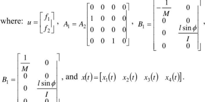
where: 2 1 f f u , 0 1 0 0 0 0 0 0 0 0 0 1 0 0 0 0 2 1 A A , 0 0 sin 0 0 0 0 1 1 I l M B , 0 0 sin 0 0 0 0 1 1 I l M B , and x
t
x1
t x2
t x3
t x4
t
.Following the design procedure in [7] (equation 2.1 – Chapter 2), the T-S fuzzy model is represented as:
2 1 i i i i t Axt But v t x .B. Design of T-S Fuzzy Logic Controller
The fuzzy logic PDC controller for the T-S fuzzy model (23) can be designed according the design procedure in [7] (equation 2.23 – Chapter 2), having the form:
t Fx t u v t 1 1, : 1 THEN is IF rule Control t Fx t u v t 2 2, : 2 THEN is IF rule Control (24)
From (23), it is obvious that the design process depends on the local feedback gains F and 1 F , which can be 2
obtained if there is a feasible solution to the LMI stability design conditions given in [7] (equations 3.15 and 3.16 – Chapter 3).
The linear matrix inequalities, adequate for the T-S fuzzy model (23) and the PDC control scheme (23), are given in the form:
0 0 0 0 1 2 2 1 2 1 1 2 2 2 1 1 2 2 2 2 2 2 1 1 1 1 1 1 M B B M M B B M X A XA X A XA M B B M X A XA M B B M X A XA X T T T T T T T T T T T T
where the feedback gains F (i i1,2) and the common
matrix P can be derived according the equations:
1
1,
X F M X
P i i , (25)
using the resulting values of X and M . i
Using the LMI toolbox in MATLAB the matrices P and Fi (i1,2) are calculated as:
0 0 0 0 0 0 0 0 0 0 0 0 0 0 0 7171 1 106 . P 7399 . 4 1278 . 12 0 0 0 0 0 0 1 F 7399 . 4 1278 . 12 0 0 0 0 0 0 2 F
Even though the solution seems to be feasible, this controller can not stabilize the system and achieve the control purpose. This was expected, as the hovercraft vehicle is typical nonholonomic system, and it can not be stabilised with any type of feedback continuous control law. Moreover, this is visible from the fact that:
0 0 sin 0 0 0 0 0 2 1 I l B t v i i i , for
t 0.This means that the first control input f1
t nevercontributes for achieving the control purpose. Given that, if the initial conditions are
Tx0 0 1 0 1.5708 , only
control input f2
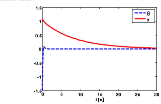
t influence the system performance,which tries to turn the vehicle from state /2 into the state 0, but y1, t . This is shown on Fig. 7.
Figure 7. Simulation results using the PDC controller for the T-S fuzzy model, for the hovercraft vehicle, for initial conditions
Tx0 0 1 0 1.5 and ( M=0.1, /4, I=0.5, l=0.1).
In the next Section we will show that the control purpose will be achieved by designing the switched fuzzy model based controller.
VII. T-S SWITCHED FUZZY CONTROLLER DESIGN FOR A
HV
In this section we will use the proposed simulation algorithms from Section IV (Fig. 2 and Fig. 3), in order to build switched fuzzy controller for the hovercraft-vehicle as a typical nonholonomic system. After synthesizing the appropriate local controllers we can build Simulink model (Fig. 4) and explore the performance of the given control system. This scheme for constructing the simulation environment can also be used for other nonlinear systems.
A. Switched Fuzzy Model
The switched fuzzy model that we will derive (according to the procedure represented on Fig. 2) will satisfy the form of the switched fuzzy model with levels of structure, given with the equations (1).
To make a switched fuzzy model for the nonlinear system (18), assume that
t
179 179
. We divide the premisevariable space into three regions with nonnegative constant
d (in [23] we have shown that the state-space partitioning
into different regions has considerable influence to the control performance of the switched fuzzy system). Therefore, the switched fuzzy model has three regions (Region 1-3) according to the premise variable . The local
tnonlinear dynamics in each region is represented by a T-S fuzzy model. We will use sector nonlinearity concept ([7]) to determine the local linear models in every region. ()
Region 1 (
t d): In this region (
t
d 179
), thenonlinear function sin
t can be rewritten as
2 1 1 1 sin i i i t a h t . Since
2 1 1 1 i i t h , the membership functions
12 11 12 11 sin a a a t t h and
12 11 11 12 sin a a t a t h ,where a111 and a12sin
1790 0.01.Region 2 (d
t d):In this region, we fix the first input, i.e. f1
t C, where C is a positive constant. This implies
CM t t
y sin . The
nonlinear function sin
t can be rewritten as t h t a t i i i
2 1 2 2 sin . Since
2 1 2 1 i i t h , the membership functions
22 21 22 21 sin a a a t t t h and
22 21 21 22 sin a a t t a t h , where a211 and a22sin
d /d.Region 3 (
t d): In this region (
t
179 d
)thenonlinear function sin
t can be rewritten as
2 1 3 3 sin i i i t a h t . Since
2 1 3 1 i i t h , the membership functions
32 31 32 31 sin a a a t t h and
32 31 31 32 sin a a t a t h ,where a311 and a32sin
1790
0.01.By aggregating the above results, according the relation (1), we construct the following switched fuzzy model for the hovercraft model (18): t A x t B u t x t h t t u B t x A t x t h t d t 12 12 12 11 11 11 , : 2 , : 1 , : 1 THEN e IF Rule Plant Local THEN e IF Rule Plant Local THEN IF Rule Region t A x t B u t x t h t t u B t x A t x t h t d t d 22 22 22 21 21 21 , : 2 , : 1 , : 2 THEN e IF Rule Plant Local THEN e IF Rule Plant Local THEN -IF Rule Region t A x t B u t x t h t t u B t x A t x t h t d t 32 32 32 31 31 31 , : 2 , : 1 , : 3 THEN e IF Rule Plant Local THEN e IF Rule Plant Local THEN IF Rule Region (26) where
t f t f t u 2 1 and
t x t x t x t x t x 1 2 3 4 , 0 1 0 0 0 0 0 0 0 0 0 1 0 0 0 0 32 31 12 11 A A A A , 0 1 0 0 0 0 0 0 0 0 0 1 0 0 0 21 21 a M C A , 0 1 0 0 0 0 0 0 0 0 0 1 0 0 0 22 22 a M C A , 0 0 sin 0 0 0 0 1 11 11 I l a M B , 0 0 sin 0 0 0 0 1 12 12 I l a M B , 0 0 sin 0 0 0 0 0 22 21 I l B B , 0 0 sin 0 0 0 0 1 31 31 I l a M B , 0 0 sin 0 0 0 0 1 32 32 I l a M B .The defuzzification is carried out according the relation (3), whereas for this case we get:
3 1 2 1 i l il il il i t h t A xt B ut t x (27) . . , 0 0 , 1 1 w o t t , . . , 0 , 1 2 w o d t d t ,
. . , 0 , 1 3 w o d t t .B. Controller Design via Switching PDC
The switching fuzzy controller of PDC type for the switched fuzzy model (26) can be designed according the relation (7), having the form:
t F x t u t h t t x F t u t h t d t 12 12 11 11 , : 2 , : 1 , : 1 THEN is IF Rule Control Local THEN is IF Rule Control Local THEN IF Rule Region t F x t u t h t t x F t u t h t d t d 22 22 21 21 , : 2 , : 1 , : 2 THEN is IF Rule Control Local THEN is IF Rule Control Local THEN IF Rule Region t F x t u t h t t x F t u t h t d t 32 32 31 31 , : 2 , : 1 , : 3 THEN is IF Rule Control Local THEN is IF Rule Control Local THEN IF Rule Region (28)
The overall fuzzy controller is obtained according the relation (8), and in this case it has the form:
3 1 2 1 i l il il i zt h zt F xt t u (29)From (29), it is obvious that the design process depends on the local feedback gains F , which can be obtained if il
there is a feasible solution to the LMI stability conditions given with Theorem 2.
The linear matrix inequalities, adequate for the switched fuzzy model (23) and the PDC control scheme (23), are given in the form:
0 0 0 3 Re % 0 0 0 2 Re % 0 0 0 1 Re % 0 31 32 32 31 32 31 31 32 32 32 31 31 32 32 32 32 32 32 31 31 31 31 31 31 21 22 22 21 22 21 21 22 22 22 21 21 22 22 22 22 22 22 21 21 21 21 21 21 11 12 12 11 12 11 11 12 12 12 11 11 12 12 12 12 12 12 11 11 11 11 11 11 M B B M M B B M X A XA X A XA M B B M X A XA M B B M X A XA gion M B B M M B B M X A XA X A XA M B B M X A XA M B B M X A XA gion M B B M M B B M X A XA X A XA M B B M X A XA M B B M X A XA gion X T T T T T T T T T T T T T T T T T T T T T T T T T T T T T T T T T T T T (30)
where the feedback gains F il (i1,2,3, 2l1, ) and the
common matrix P can be derived according the equations:
1
1,
X F M X
P il il , (31)
using the resulting values of X and Mi from (30).
Using the proposed simulation scheme on Fig. 3, i.e. using the LMI toolbox in MATLAB, we have got feasible solution for the values of matrices P and Fil (i1,2,3,
2 , 1 l ), in the form: 1416 . 0 0124 . 0 0106 . 0 0942 . 0 0124 . 0 0016 . 0 0009 . 0 0083 . 0 0106 . 0 0009 . 0 0016 . 0 0097 . 0 0942 . 0 0083 . 0 0097 . 0 0866 . 0 P 1942 . 2 1934 . 0 1645 . 0 4596 . 1 0031 . 0 0003 . 0 0003 . 0 0028 . 0 103 11 F 1937 . 2 1933 . 0 1644 . 0 4591 . 1 0091 . 0 0008 . 0 0010 . 0 0085 . 0 103 12 F 5663 . 1 1380 . 0 0908 . 0 8826 . 0 0 0 0 0 103 21 F 5667 . 1 1381 . 0 0999 . 0 8830 . 0 0 0 0 0 103 22 F 1958 . 2 1935 . 0 1646 . 0 4610 . 1 0030 . 0 0003 . 0 0003 . 0 0028 . 0 103 31 F 1937 . 2 1933 . 0 1644 . 0 4592 . 1 0091 . 0 0008 . 0 0010 . 0 0085 . 0 103 32 F
Fig. 8 shows the values of the control variables y and , using the switching PDC controller. In this case, unlike the case when ordinary T-S fuzzy controller is used, it is clear that the control purpose (lim
0
yt
t and tlim
t 0) isachievable.
Figure 8. .Values for and y, when the LMI conditions according the Theorem 2 are used. Initial conditions are
Tx0 0 1 0 1.5 and ( M=0.1, /4, I=0.5, l=0.1, C=0.5, d/50). 0 0.5 1 1.5 -2000 -1500 -1000 -500 0 500 1000 1500 2000 t [s] Fr Fl 0 0.5 1 1.5 1 1.5 2 2.5 3 t [s] a) b)
Showing this it is obvious that the use of switching fuzzy controllers is worthwhile in comparison of ordinary T-S fuzzy controllers which are continuous feedback control laws. However, if we view the control effort, i.e. the values of fR
t and fL
t , (see Fig. 9-a), it is obvious that theyhave very high amplitudes. The respective switching signal that selects the appropriate region during the control period is shown on Fig. 9- b.
Figure 10. .Values for y, using the control signals, shown on Fig. 12.
Figure 11. .Values for , using the control signals, shown on Fig. 12.
For constraining the control inputs fR
t and fL
t , wecan use the LMI conditions given with (17). Please note that the LMI conditions (17) depend on the initial conditions, so whenever we would like to change the initial conditions it would be necessary to recalculate the feedback control gains according the design process on Fig. 3.
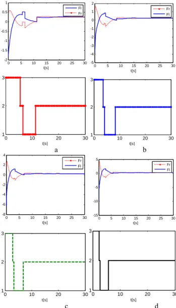
Fig. 10 and Fig. 11 show the values of the control variables for the four different constraint inputs, given on Fig. 12-a,b,c,d. It is obvious that as much as the control inputs are constraint, as hard as the control purpose is achieved. 0 5 10 15 20 25 30 -2 -1.5 -1 -0.5 0 0.5 1 t[s] Fl Fr 0 5 10 15 20 25 30 -5 -4 -3 -2 -1 0 1 2 t[s] Fr Fl 0 10 20 30 1 2 3 t[s] 0 10 20 30 1 2 3 t[s] a b 0 5 10 15 20 25 30 -8 -6 -4 -2 0 2 4 t[s] Fr Fl 0 5 10 15 20 25 30 -15 -10 -5 0 5 t[s] Fr Fl 0 10 20 30 1 2 3 t[s] 0 10 20 30 1 2 3 t[s] c d
Figure 12. .Control inputs fR
t and fL
t and the appropriate switchingsignal, when the joined LMI conditions according the Theorem 2 and Theorem 4 are used. Initial conditions are
Tx0 0 1 0 1.5 and ( M=0.1, /4, I=0.5, l=0.1, C=0.5, d/50).
VIII. CONCLUSION
We have shown that the proposed mechanism for modelling and simulation of the performance of switched fuzzy systems is applicable for building and simulating the switched fuzzy control of the hovercraft vehicle, whereas we expect that these concepts can be used for building and simulating the switched fuzzy control of other nonlinear systems. Also, with the derived simulation results that show the feasibleness of the use of switching fuzzy controllers for the systems that are not stabilizable with any continuous feedback control laws, we believe that this type of control will be used in solving many control problems that were not
0 5 10 15 20 25 30 -1.6 -1.4 -1.2 -1 -0.8 -0.6 -0.4 -0.2 0 0.2 t[s] Theta [rad] Input a Input b Input c Input d 0 5 10 15 20 25 30 0 5 10 15 t [s] y Input a Input b Input c Input d
solvable with other types of controllers. Among many questions that arise considering the performance of switched fuzzy systems is the state-space partitioning. In [23] we have shown that the state-space partitioning into different regions has considerable influence to the control performance of the switched fuzzy system.
ACKNOWLEDGMENT
This research was part of the FANEN Scientific Research Project, financed by the Ss Cyril and Methodius University in Skopje, R. Macedonia, Faculty of Electrical Engineering and Information Technologies (Tatjana Kolemishevska-Gugulovska, Principal investigator - 2011 – 2012, contracted on 20.1.2011).
REFERENCES
[1] D. Liberzon. Switching in Systems and Control. Boston, MA: Birkhauser, 2003.
[2] Z. Sun and S. S. Ge. Switched Linear Systems - Control and Design. London: Springer, 2005.
[3] H. Lin and P. J. Antsaklis. “Stability and Stabilizability of Switched Linear Systems: A Survey of Recent Results.” IEEE Transactions on Automatic Control, vol. 54, no. 2, Feb. 2009.
[4] J. Zhao and G. M. Dimirovski. “Quadratic stability of a Class of Switched Nonlinear Systems.” IEEE Transactions on Automatic Control, vol. 49, no. 4, Apr. 2004.
[5] G. Feng. “A Survey on Analysis and Design of Model-Based Fuzzy Control Systems.” IEEE Transactions on Fuzzy Systems, vol. 14, no. 5, Oct. 2006.
[6] O. Kaynak, K. Erbatur and M. Ertugnrl. “The Fusion of Computationally Intelligent Methodologies and Sliding-mode Control - a Survey.” IEEE Transactions on Industrial Electronics, vol. 48, no. 1, pp. 4–17, Feb. 2001.
[7] K. Tanaka and H. O. Wang. Fuzzy Control Systems Design and Analysis: A Linear Matrix Inequality Approach. New York: John Wiley & Sons, 2001.
[8] R. Palm and D. Driankov. “Fuzzy switched hybrid systems - modelling and identification.” in Proc. of the IEEE ISIC/CIRA/ISAS Joint Conference, Gaithersburg, MD, Sep. 14-17, 1998, pp. 130-135. [9] K. Tanaka, M. Iwasaki and H. O. Wang. “Stabilization of switching
fuzzy systems.” in Proc. of Asian Fuzzy System Symposium, 2000. [10] K. Tanaka, M. Iwasaki and H. O. Wang. “Stable switching fuzzy
control and its application to a hovercraft type vehicle.” in Proc. of the Ninth IEEE International Conference on Fuzzy Systems, 2000, vol. 2, pp. 804–809.
[11] K. Tanaka, M. Iwasaki and H. O. Wang. “Stability and smoothness conditions for switching fuzzy systems.” in Proc. of the 2000 American Control Conference, Chicago, Ilinois, Jun. 2000, pp. 2474-2478.
[12] K. Tanaka, M. Iwasaki and H. O. Wang. “Switching Control of an R/C Hovercraft: Stabilization and Smooth Switching.” IEEE
Transactions on Systems, Man, and Cybernetics Part B: vol. 31, no. 6, Dec. 2001.
[13] H. Ohtake, K. Tanaka and H. O. Wang. “A construction method of switching Lyapunov function for nonlinear systems.” in Proc. of the 2002 IEEE International Conference on Fuzzy System, 2002, pp. 221-226.
[14] H. Ohtake and K. Tanaka. “Switching Model Construction and Stability Analysis for Nonlinear Systems.” Journal of Advanced Computational Intelligence and Intelligent Informatics, vol.10, no.1, 2006.
[15] H. Yang, J. Feng and J. Zhao. “Stability of a class of fuzzy systems based on fuzzy controller switching.” in Proc. of the 6th World
Congress on Intelligent Control and Automation, Dalian, China, Jun. 21-23, 2006, vol. 1, pp. 685-689.
[16] H. Yang, G. M. Dimirovski and J. Zhao. “Switched fuzzy systems: representation modelling, stability analysis, and control design.” in Proc. of the 3rd International IEEE Conference on Intelligent Systems, London, England, Sep. 4-6, 2006, pp. 306-311.
[17] H. Yang, G. M. Dimirovski and J. Zhao. “Switched Fuzzy Systems: Representation Modelling, Stability Analysis and Control Design.” in Studies in Computational Intelligence 109, Berlin Heidelberg, DE: Springer-Verlag, 2008, pp. 155-168.
[18] H. Yang, H. Liu, G. M. Dimirovski and J. Zhao. “Stabilization control for a class of switched fuzzy discrete-time systems.” in Proc. of the 2007 IEEE International Conference on Fuzzy Systems, London, England, Jul. 23-28, 2007, pp. 1345-1350.
[19] H. Yang, G. M. Dimirovski and J. Zhao. “A state feedback H∞ control design for switched fuzzy systems.” in Proc. of the 4th IEEE
International Conference on Intelligent Systems, Varna, Bulgaria, Sep. 6-8, 2008.
[20] V. Ojleska and G. Stojanovski. “Switched fuzzy systems: overview and perspectives.” in Proc. of the 9th
International PhD Workshop on Systems and Control – A Young Generation Viewpoint, Izola, Slovenia, Oct. 1-3, 2008.
[21] V. Ojleska, T. K.-Gugulovska and G. M. Dimirovski. “A survey on modelling, analysis and design of switched fuzzy control systems.” in Preprints of IFAC WS DECOM 2009, Ohrid, Macedonia, Sep. 26-29, 2009. Also to apear in IFAC Papers On-Line 2011 in the Proceedings of DECOM-IFAC-09.
[22] V. Ojleska, T. K.-Gugulovska and G. M. Dimirovski. “Switched fuzzy control systems: exploring the performance in applications.” in Proc. of the 2010 UKSim Fourth European Modelling Symposium on Computer Modelling and Simulation, EMS 2010, Pisa, Italy, Nov. 17-19, pp. 37-42. [23] V. Ojleska, T. K.-Gugulovska and G. M. Dimirovski. “Influence of
the State Space Partitioning into Regions when Designing Switched Fuzzy Controllers.” Facta Universitatis Series Automatic Control and Robotics, vol. 9, no 1, pp. 103-112, 2010.
[24] S. Boyd, L. El Ghaoui, E. Feron and V. Balakrishnan. Linear Matrix Inequalities in Systems and Control Theory. Philadelphia: SIAM, 1994.
[25] H. O. Wang, K. Tanaka and M. Griffin. “Parallel distributed compensation of nonlinear systems by Takagi and Sugeno’s Fuzzy Model.” in Proc. of FUZZ-IEEE’95, 1995, pp. 531-538.
![Figure 1. Sketch map of switched fuzzy system [19].](https://thumb-eu.123doks.com/thumbv2/9libnet/4078348.58296/2.892.465.794.266.332/figure-sketch-map-of-switched-fuzzy-system.webp)