133
Araştırma Makalesi - Research Article
Artırımlı Sosyal Öğrenme Tabanlı Diferansiyel Gelişim
Algoritması
Serdar Özyön
1*Geliş / Received: 28/12/2019 Revize / Revised: 08/02/2020 Kabul / Accepted: 14/02/2020
ÖZ
Bu çalışmada, literatürde yer alan optimizasyon algoritmaları arasında çok güçlü bir yere sahip olan diferansiyel gelişim algoritmasının (DE) geliştirilmesi ve iyileştirilmesi üzerine çalışılmıştır. DE’ye daha önce farklı optimizasyon algoritmalarına uygulanan ve olumlu geri dönüşler alınan artırımlı sosyal öğrenme yapısı (ISL) farklı yaklaşımlarla entegre edilerek, algoritma iyileştirilmiştir. Yapılan bu iyileştirmelerde DE, belirlenen minimum sayıda bireyle aramaya başlatılmış, belirli adımlarda farklı yaklaşımlarla popülasyona yeni bireyler eklenmiş, belirlenen maksimum popülasyon sayısında birey ekleme işlemi sonlandırılmış ve durdurma kriteri sağlanana kadar bu popülasyon sayısıyla aramaya devam edilmiştir. DE’nin yeni bir versiyonu olarak ortaya çıkarılan iyileştirilmiş bu algoritmaya artırımlı diferansiyel gelişim algoritmasının (IDE) adı verilmiştir. Çalışmada öne çıkan diğer bir amaç ISL yapısında en iyi birey ekleme yönteminin belirlenmesidir. Bu amaçla, DE’ye birey ekleme işlemi beş farklı yaklaşımla yapılmıştır. DE ve bu çalışmada geliştirilen IDE algoritmalarıyla, 13 adet, 30 boyutlu unimodal ve multimodal test fonksiyonlarının çözümleri yapılmıştır. Elde edilen sayısal sonuçlar, grafikler ve istatistiki analizler incelenerek, değerlendirmeler yapılmıştır.
Anahtar Kelimeler- Diferansiyel gelişim algoritması (DE), Artırımlı sosyal öğrenme yapısı (ISL), Unimodal ve multimodal karşılaştırma fonksiyonları, Optimizasyon.
*Sorumlu yazar iletişim: [email protected] (https://orcid.org/0000-0002-4469-3908)
134
Differential Evolution Algorithm with Incremental Social
Learning
ABSTRACTIn this study, the differential evolution algorithm (DE), which has a very strong place among the optimization algorithms in literature, has been tried to be improved and bettered. The algorithm has been bettered by integrating incremental social learning (ISL) structure, which was applied to different optimization algorithms previously with positive feedbacks, into DE. In this betterment, DE has been initiated to search with a number of determined individuals, new individuals have been added to the population with different approaches in certain levels, the process of adding individuals has been ended at the maximum population number determined and the search has been continued with this population number until the stopping criterion has been provided. This new bettered algorithm which has been revealed as a new version of DE has been called Incremental differential evolution algorithm (IDE). Another purpose that comes into prominence in the study is to determine the best method to add individuals in ISL structure. For this purpose, five different approaches have been used in the operation of adding individuals to DE. A set of 13 unimodal and multimodal test functions defined on a 30-dimensional space have been solved with DE and IDE algorithms improved in this study. Evaluations have been made by examining the obtained numerical results, graphics and statistical analyses.
Keywords- Differential Evolution Algorithm (DE), Incremental social learnings (ISL), Unimodal and multimodal benchmark functions, Optimization.
135 I. INTRODUCTION
In today’s extremely competitive world, people are trying to obtain maximum efficiency and profit from a limited amount of existing sources. For instance, in engineering design, the selection of the design variables with the possible lowest cost, which meet all the design requirements, is in question. Meanly the main purpose is to conform to the main standards and at the same time to obtain good economic results. The purpose of the optimization is this, as well.
As a definition, “optimization” expresses the study of the problems which want to decrease a function to the least or to carry it to the highest level (minimize or maximize a function) by choosing the values of the variables in a permitted set systematically Many studies have been done in literature, in accordance with this definition, in order to develop more effective and efficient optimization algorithms. Among these studies, some optimization algorithms, which have gained a wide place in literature can be mentioned as the following: genetic algorithm [1], simulated annealing [2], differential evolution [3], particle swarm optimization [4], harmony search [5], artificial bee colony [6], ant colony optimization [7], gravitational search algorithm [8], bacterial foraging optimization algorithm [9], charged system search [10], colliding bodies optimization [11], big bang-big crunch method [12], black hole algorithm [13], water-wave optimization [14], the whale optimization algorithm [15], cuckoo optimization algorithm [16], moth-flame optimization algorithm [17], crow search algorithm [18], a sine cosine algorithm [19], optics inspired optimization [20], multi-verse optimizer [21], radial movement optimization [22], grey wolf optimizer [23] and symbiotic organisms search [24].
On the other hand, applying these developed algorithms to real world problems has become a focus point of many researches, as well. These algorithms have contributed to the solution of many problems in applied mathematics, engineering, medicine, economics and in different fields of other sciences. These methods are also widely used in the design of different systems in civil, mechanical, electrical and industrial engineering. Depending on the increase in the areas of usage, it has become necessary to change the present situation of the algorithms into a faster and more decisive structure. Therefore, improvements have been provided by integrating many different structures into algorithms. One of these methods is the use of incremental social learning (ISL) structure together with algorithm [25]. In population-based optimization algorithms, ISL structure is based on the basis of adding new individuals to the population in time. The algorithm with this structure, starts to search with a small number of individuals in the solution search space, new learning is aimed at by adding new individuals, which communicate with the already existing individuals, to the population. In the literature review, ISL structure has been used successfully in four different optimization algorithms. These are particle swarm optimization [26,27], ant colony optimization [28], artificial bee colony [29,30] and gravitational search [31] algorithms. When these studies are examined, it has been seen that ISL structure has created positive effects on the performances of the algorithms.
In this study, it is aimed to improve the performance of DE, which is shown among the best optimization algorithms in literature, by the use of it together with ISL structure and to change it into a faster and more decisive structure. For this reason, unlike other studies, ISL has been integrated into DE in five different ways. High dimensional unimodal and multimodal test functions have been solved with the created algorithms for each approach and the obtained results have been discussed.
II. DIFFERENTIALEVOLUTIONALGORITHM(DE)
DE, which is a genetic algorithm-based and population grounded optimization technique, was first proposed by Price and Storn in 1995. At the basis of the algorithm lies obtaining a new solution by subjecting the candidate solutions, each including a solution in itself, to the operators one by one. During these processes, mutation and crossover operators are used. If the fitness of the new individual, meanly its closeness to the solution is better than the old one, the new individual is transformed to the next population, otherwise the old individual is transformed [3,32].
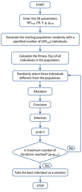
The basic algorithm parameters used in DE are the size of the population (NPmax), maximum iteration number (gmax), crossover rate (CR) and scaling factor (F). The process steps of the algorithms can be defined as variable assignment and formation of the initial population, calculation of the fitness of the individuals,
136 selection, mutation, crossover and stopping of the algorithm. The flowchart belonging to the algorithm has been given in Figure 1 [3,32].
Enter the DE parameters NPmax, CR, F, g, gmax
g=g+1
STOP
Is maximum number of iterations reached? (g=gmax)
No Yes START Mutation Crossover Selection
Generate the starting population randomly with a specified number of (NPmax) individuals.
Calculate the fitness F(xi) of all individuals in the population.
Take the best individual as a solution. Randomly select three individuals
different from the population.
137 Three candidate solutions are required in order to generate a new candidate solution in DE. The generation of the initial population formed of NP numbered, D dimensional candidate solutions is done from the equation below. ( ) ( ) ( ) , , =0= + [0,1].( − ) l u l j i g j j j j x x rand x x (1)
xj,i,g, taking place where shows j parameter of i candidate solution in g population while ( ( )l , ( )u )
j j
x x
shows the lower and upper limits belonging to the variables [3,32].
After the formation of the population, mutation process takes place. Mutation is to make random changes on the genes of the selected candidate solutions. Apart from the present candidate solution three candidate solutions different from each other are chosen for mutation process in the main structure of DE (r1, r2, r3). The difference of the first two is taken and multiplied with F. F is generally taken as a value changing between 0~2. Weighted difference candidate solution is summed up to the third candidate solutions. The mathematical expression of the mutation process applied in this study has been shown in equation (2). Different kinds of mutations are also present for DE in different studies [3,32,33].
3 1 2
, ,+1= , , + .( , , − , , ) j i g j r g j r g j r g
n x F x x (2)
where nj,i,g+1 shows the intermediate candidate solutions subjected to mutation and crossover, r1, r2, r3 show the randomly selected candidate solutions that will be usedin the generation of new candidate solution
1,2,31, 2, 3, ,
r NP , r1 r2 r3 i.
New candidate solution (ui,g+1) is generated by using the difference candidate solution obtained as a result of mutation and xi,g candidate solution. The genes for the trial candidate solution are selected from difference candidate solution with CR probability and from the present candidate solution with (1-CR) probability. j=jrand condition, is used to guarantee the removal of at least one gene from the newly generated candidate solution. A randomly selected gene at the point of j=jrand, is selected from nj,i,g+1 without looking at CR value [3,32]. , , 1 , , 1 , , [0,1] + + = = j n g rand j u g j i g x if rand CR or j j x x otherwise (3)
A new candidate solution (trial) has been obtained by using three different candidate solutions together with the objective candidate solution and with the use of mutation and crossover operators. The candidate solution, which will be transferred to the new population (g=g+1), is determined by looking at its fitness value. The fitness value of the objective candidate solution is already known. The candidate solution whose fitness is high among others is transferred to the new population. The iterations continue until it becomes (g=gmax); when it becomes gmax, the best individual in the present population is taken as solution [3,32].
, 1 , 1 , 1 , 1 , ( ) ( ) + + + + = u g u g i g i g i g x if f x f x x x otherwise (4)
The purpose in algorithm is to obtain candidate solutions with better fitness values continuously and to catch the optimum value or to approximate this value. The circle is carried on until it becomes g=gmax. The stopping of the algorithm in the study depends on the defined iteration number.
III. INCREMENTALSOCIALLEARNING(ISL)
The concept of social learning (SL) is generally used to be able to make the information transfer between individuals without genetic operators. The use of this concept is very suitable for the design of
multi-138 individual systems. The reason of this is that it enables the new individuals entering into the population get information from the other experienced individuals without letting them waste time to get information individually. Theoretical models and empirical studies have shown the result that depending only on socially obtained information is not always advantageous. Providing social learning with the individuals who are wanted to be explained here only with the population is not very effective on the algorithm. It has been found that it is more beneficial to relate randomly generated individuals to individuals providing learning in the population so far. For social learning to be useful, individuals need additional time, in order to learn individually or to make novelties. This approach, which is called incremental social learning, is formed of an increasing individual population, which learns socially when it becomes a part of the main population and learns individually when it becomes a part of the population. The roof of ISL, in individual systems learning multiple, is based on the basis of adding new individuals to the system in time. Algorithms having this structure start to search in the solution search space with small number of individuals and perform a fast learning process. In the next steps, the search is continued by adding new individuals, which are made to get into contact with the present individuals in various ways, to population. Increasing population strategy is based on the observation that newly born individuals in nature learn much more skills than the adult individuals surrounding them. The basic structure of Incremental social lerning approach has been given in Figure 2 [25-31].
Figure 2. Incremental social learning (ISL) algorithm basic structure
IV. INCREMENTALDIFFERENTIALEVOLUTIONALGORITHM(IDE)
Population-based optimization algorithms generally start to search in the solution space with a certain number of individual populations formed randomly. Therefore, the location of the individuals of the firstly formed population, in the search space is very important to be able to obtain the best result. In a condition of the location of the individuals in the first randomly formed population, near local minimums, it is not possible to converge to the best result. Therefore, the risk of being caught by the local minimum points is decreased by integrating ISL structure to the algorithm doing multiple search and with adding new individuals to the system in time. The population is at first formed of a small number of individuals and a fast learning is performed. Later new individuals that get into contact with the present individuals are added to the population. An individual added to the population learns socially from the other individuals existing in the population for some time. This element of ISL is attractive, because through social learning the individuals obtain the information from more experienced individuals, without spending time to get the information individually. Thus, ISL achieves to save from the time which will be spent to teach new things to the new individuals. After adding a new individual to the population, the population needs to have a look at the new conditions again, but the individuals, which are a part of it, do not need to learn everything from the beginning [25-31].
In this study, Incremental differential evolution algorithm (IDE), which has been developed by adding ISL structure to Differential evolution algorithm (DE), is based on the principle of increasing the number of
Incremental Social Learning (ISL) Algorithm % Initilization
t=0;
%İnitialize environment Et
%İnitialize primogenial population of agents Xt
% Main loop
while Stopping criteria not met do
if Agent addition Schedule or criterion is not met then Xt+1→ilearn (Xt, Et) %Individual learning
else
Create new agent anew slearn (anew, Xt) %Social learning
Xt+1Xt U {anew}
end if
Et+1update (Et) %Update environment
tt+1
139 individuals in the population at regular intervals. An individual at a defined iteration interval (number of steps, SS) is added to the population in various ways, until the population reaches the defined maximum individual number (Nmax). In the previous ISL studies, either one way or at most three ways of individual adding approach were tried [30,31]. For the first time in this study, adding individuals to the population has been done with five different approaches. The purpose of using different approaches while adding individuals is to shed light on the following studies that will be done with ISL, about the best method of adding individual.
A. Case 1: IDE-1
In the first approach, the search in the solution space is started with the defined minimum number of individual. The number of the individuals is increased by adding another new individual, which is formed in the search space randomly at certain intervals, to the population as in equation (5). This process continues until the defined maximum individual number is completed.
' , ( )= , ( ) j New j Rand x t x t (5) ' , ( ) j New
x t j. taking place, where shows the individual newly added to the population in the iteration, and , ( )
j Rand
x t j. shows an individual that has been formed randomly in the search space in the iteration. B. Case 2: IDE-2
In this approach, the new individual that will be added to the population is selected randomly among the individuals in the population at that moment as in equation (6). This process continues with certain intervals until the maximum individual number is completed.
'
, ( )= , ( ) j New j Pop
x t x t (6)
Where xj Pop, ( )t j. expresses a randomly selected individual from the population in the iteration.
C. Case 3: IDE-3
In this approach, the best individual taking place in the population at that moment is added to the population as in equation (7) and number of individuals is increased. This process continues with certain intervals until the maximum individual number is completed.
'
, ( )= , ( ) j New j Best
x t x t (7)
where xj Best, ( )t j. expresses the best individual in the population in the iteration.
D. Case 4: IDE-4
In the fourth approach, the new individual that will be added to the population, is determined by getting an individual, randomly selected from the population, into contact with the individual having the best solution as in equation (8). This process continues with certain intervals until the maximum individual number is completed.
'
, ( )= , ( )+ [0,1] , ( )− , ( )
j New j Pop j Best j Pop
x t x t rand x t x t (8)
where rand [0,1] expresses a randomly assigned number at 0-1 interval. E. Case 5: IDE-5
140 In the fifth approach, the individual that will get into contact with the best individual in the population is formed randomly in the search space and added to the population according to equation (9). This process continues with certain intervals until the maximum individual number is completed.
'
, ( )= , ( )+ [0,1] , ( )− , ( )
j New j Rand j Best j Rand
x t x t rand x t x t (9)
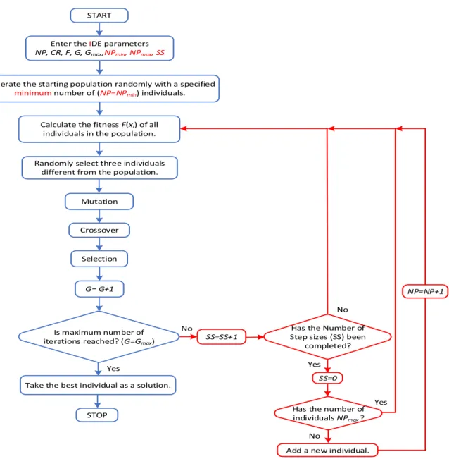
According to the previous studies, in another innovation in this study, the sentence is done in 5 different ways and determining the most suitable individual addition method. The flowchart for the IDE algorithms that have been defined in the previous parts has been given in Figure 3. In the diagram, the parameter and process differences of IDE algorithm from DE algorithm, whose flowchart has been given in Figure 1, have been shown in red.
Enter the IDE parameters NP, CR, F, G, Gmax,NPmin, NPmax, SS
START
G= G+1
STOP
Is maximum number of iterations reached? (G=Gmax)
Yes Mutation
Crossover
Selection
Generate the starting population randomly with a specified
minimum number of (NP=NPmin) individuals.
Calculate the fitness F(xi) of all individuals in the population.
Take the best individual as a solution. Randomly select three individuals
different from the population.
SS=SS+1
No Has the Number of
Step sizes (SS) been completed?
No
Yes
NP=NP+1
Has the number of individuals NPmax ?
No
Yes SS=0
Add a new individual.
141
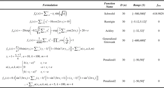
V. UNIMODALANDMULTIMODALTESTFUNCTIONS
The developed algorithms (IDE) have been applied to 13, 30 dimensional unimodal and multimodal test functions, which were solved with different algorithms in literature previously, in order to evaluate the performance of them. These functions have been given in Table 1 and 2 as two groups.
Table 1. Unimodal test functions
Formulation Function Name D (n) Range (S) fmin
2 1( ) 1 n i i f x =
=x Sphere 30 [ 100,100]− n 0 2( ) 1 1 n n i i i i f x =
= x +
= x Schwefel 2.22 30 [ 10,10]− n 0(
)
2 3( ) 1 1 n i j i j f x =
= =x Schwefel 1.22 30 [ 100,100]− n 0
4( ) max i,1 f x = x i n Maximization 30 [ 100,100]− n 0(
)
2 ( ) 1 2 2 5( ) 1 100 1 1 n i i i i f x =
=− x+ −x + x− Rosenbrock 30 [ 30,30] n − 0 ( )2 6( ) 1[ 0.5] n i i f x =
= x+ Step 30 [ 100,100]− n 0 4 7( ) 1 [0,1) n i if x =
=ix +random Quartic noise 30 [ 1.28,1.28]− n0
Table 2. Multimodal test functions
Formulation Function
Name D (n) Range (S) fmin
( )
8( ) 1 sin n i i f x =
= −x x Schwefel 30 [ 500,500]− n -418.9829.n 2 9( ) 1 10 (2 ) 10 n i i i f x =
=x − cos x + Rastrigin 30 [ 5.12,5.12]− n 0 2 10 1 1 1 1( ) 20exp 0.2 in i exp in cos(2 i) 20
f x x x e n = n = = − − − + +
Ackley 30 [ 32,32] n − 0 2 11 1 1 1 ( ) cos 1 4000 n n i i i i x f x x i = = = − +
Generalized Griewank 30 [ 600,600] n − 0
1 2 2
1 12( ) 10sin( 1) 1( 1) 1 10sin ( 1) 1 ( , , , ) 1 1 , 10, 100, 4 4 ( ) ( , , , ) 0 -( ) n n i i i i i i i m i i i i m i i f x y y y u x a k m n x y a k m k x a x a u x a k m a x a k x a x a − − + = = = + − + + + = + = = = − = − − −
Penalized1 30 [ 50,50]− n 0
2 2 2 2 2
13 1 1 1( ) 0.1 sin (3 ) ( 1) 1 sin (3 1) ( 1) 1 sin (2 ) ... ( , , , ), 5, 100, 4 n i i n n i n i i f x x x x x x u x a k m a k m = = = + − + + + − + + = = =
Penalized2 30 [ 50,50] n − 0In the tables D shows the dimension of the functions, (S) search ranges, and fmin shows the minimum values of the functions. The functions taking place in the tables are high dimensional functions or functions with
142 wide search space. Functions in Table 1 are unimodal functions with only one minimum point, and functions in Table 2 are multimodal functions with a lot of local minimum points.
VI. NUMERICALRESULTS
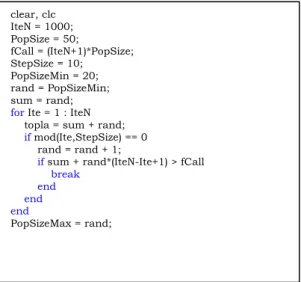
In the study, the solutions of the test functions in Table 1 and 2 have been done with DE and IDE approaches under the same circumstances with the same sizes and parameters in order to be able to make an accurate comparison of the algorithms in terms of performance. IDE parameters given in Figure 3 the calculation of the minimum agent number (Nmin), and the maximum agent number (Nmax) according to step number (SS) have been done with the subprogram the code of which is given in Figure 4, in order that all algorithms can be able to search with an equal number of function calls (fCall) [31]. After these calculations DE and IDE parameter values, which have been used for the solution of all functions in the study have been given in Table 3. In this study the solution of the test functions have been done in MATLAB R2015b by using a workstation with Intel Xeon E5-2637 v4 3.50 GHz processor and 128 GB RAM memory.
Figure 3. The flowchart of IDE
Table 3. DE and IDE parameter values
Algorithm (IteN) (N) (fCall) (SS) (Nmin) (Nmax) (F) (CR)
DE 1000 - 50000 10 20 57 0.8 0.4 IDE 50 - - -
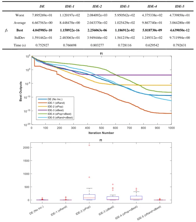
The solution values obtained for f1 function in 30 runs have been given in Table 4, the convergence graphics belonging to the best solution and the box plots of 30 solutions have been given in Figure 5. The horizontal axis in the boxplots shows the algorithms designed according to the method of adding different individuals, and the vertical axis shows the best values obtained from 30 runs with these algorithms.
clear, clc IteN = 1000; PopSize = 50; fCall = (IteN+1)*PopSize; StepSize = 10; PopSizeMin = 20; rand = PopSizeMin; sum = rand;
for Ite = 1 : IteN topla = sum + rand; if mod(Ite,StepSize) == 0 rand = rand + 1;
if sum + rand*(IteN-Ite+1) > fCall break
end
end end
143 Table 4. The data obtained for f1 in 30 runs
DE IDE-1 IDE-2 IDE-3 IDE-4 IDE-5
f1
Worst 7.895269e+01 1.120197e+02 2.084092e+03 5.950562e+02 4.375338e+02 4.739850e+01 Average 6.667563e+00 8.448470e+00 2.043370e+02 1.025429e+02 9.867740e+01 3.064280e+00
Best 4.045985e-10 1.158922e-16 2.256063e-06 1.186912e-02 5.818730e-09 4.639050e-12
StdDev 1.591462e+01 2.483063e+01 3.949446e+02 1.561219e+02 1.249312e+02 9.711994e+00 Time (s) 0.752927 0.766698 0.803277 0.728116 0.629542 0.792631
Figure 5. Convergence curves belonging to the best solutions obtained for f1 and box plots
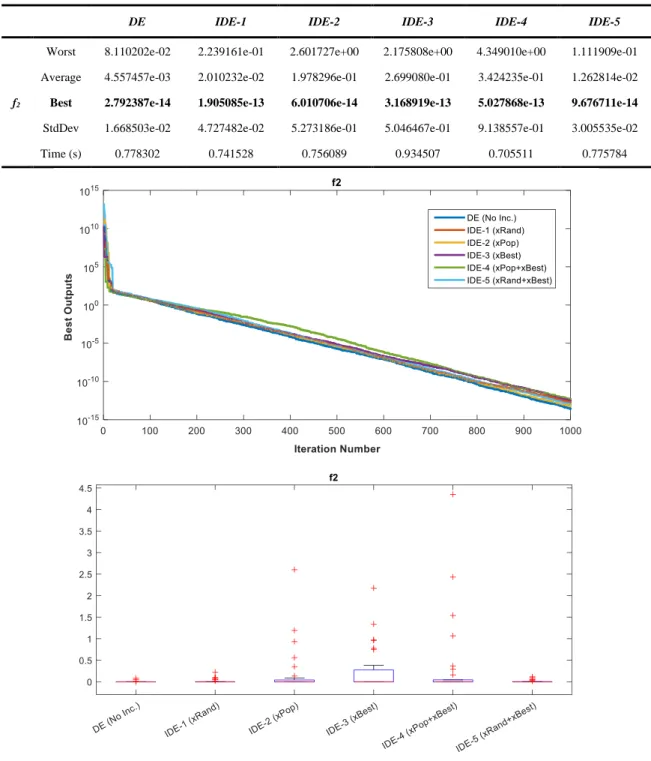
The solution values obtained for f2 function in 30 runs have been given in Table 5, the convergence graphics belonging to the best solution and the box plots of 30 solutions have been given in Figure 6.
144 Table 5. The data obtained for f2 in 30 runs
DE IDE-1 IDE-2 IDE-3 IDE-4 IDE-5
f2
Worst 8.110202e-02 2.239161e-01 2.601727e+00 2.175808e+00 4.349010e+00 1.111909e-01 Average 4.557457e-03 2.010232e-02 1.978296e-01 2.699080e-01 3.424235e-01 1.262814e-02
Best 2.792387e-14 1.905085e-13 6.010706e-14 3.168919e-13 5.027868e-13 9.676711e-14
StdDev 1.668503e-02 4.727482e-02 5.273186e-01 5.046467e-01 9.138557e-01 3.005535e-02 Time (s) 0.778302 0.741528 0.756089 0.934507 0.705511 0.775784
Figure 6. Convergence curves belonging to the best solutions obtained for f2 and box plots
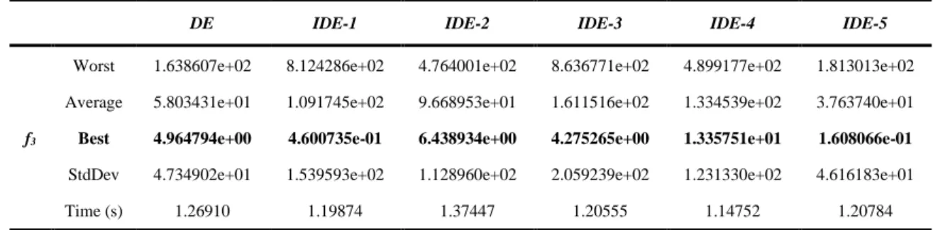
The solution values obtained for f3 function in 30 runs have been given in Table 6, the convergence graphics belonging to the best solution and the box plots of 30 solutions have been given in Figure 7.
145 Table 6. The data obtained for f3 in 30 runs
DE IDE-1 IDE-2 IDE-3 IDE-4 IDE-5
f3
Worst 1.638607e+02 8.124286e+02 4.764001e+02 8.636771e+02 4.899177e+02 1.813013e+02 Average 5.803431e+01 1.091745e+02 9.668953e+01 1.611516e+02 1.334539e+02 3.763740e+01
Best 4.964794e+00 4.600735e-01 6.438934e+00 4.275265e+00 1.335751e+01 1.608066e-01
StdDev 4.734902e+01 1.539593e+02 1.128960e+02 2.059239e+02 1.231330e+02 4.616183e+01
Time (s) 1.26910 1.19874 1.37447 1.20555 1.14752 1.20784
Figure 7. Convergence curves belonging to the best solutions obtained for f3 and box plots
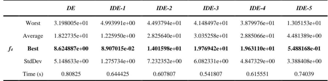
The solution values obtained for f4 function in 30 runs have been given in Table 7, the convergence graphics belonging to the best solution and the box plots of 30 solutions have been given in Figure 8.
146 Table 7. The data obtained for f4 in 30 runs
DE IDE-1 IDE-2 IDE-3 IDE-4 IDE-5
f4
Worst 3.198005e+01 4.993991e+00 4.493794e+01 4.148497e+01 3.879976e+01 1.305153e+01 Average 1.822735e+01 1.225950e+00 2.825640e+01 3.035258e+01 2.885066e+01 4.481389e+00
Best 8.624887e+00 8.907015e-02 1.401598e+01 1.976942e+01 1.963110e+01 5.488168e-01
StdDev 5.148633e+00 1.275734e+00 7.232352e+00 6.082331e+00 4.847329e+00 3.388408e+00 Time (s) 0.80825 0.644425 0.607807 0.541807 0.615551 0.74039
Figure 8. Convergence curves belonging to the best solutions obtained for f4 and box plots
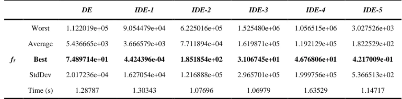
The solution values obtained for f5 function in 30 runs have been given in Table 8, the convergence graphics belonging to the best solution and the box plots of 30 solutions have been given in Figure 9.
147 Table 8. The data obtained for f5 in 30 runs
DE IDE-1 IDE-2 IDE-3 IDE-4 IDE-5
f5
Worst 1.122019e+05 9.054479e+04 6.225016e+05 1.525480e+06 1.056515e+06 3.027526e+03 Average 5.436665e+03 3.666579e+03 7.711894e+04 1.619871e+05 1.192129e+05 1.822529e+02
Best 7.489714e+01 4.424396e-04 1.851854e+02 3.106745e+01 4.676806e+01 4.217009e-01
StdDev 2.017236e+04 1.627054e+04 1.216888e+05 2.965701e+05 1.999756e+05 5.366513e+02
Time (s) 1.28787 1.30343 1.07696 1.06979 1.63529 1.14717
Figure 9. Convergence curves belonging to the best solutions obtained for f5 and box plots
The solution values obtained for f6 function in 30 runs have been given in Table 9, the convergence graphics belonging to the best solution and the box plots of 30 solutions have been given in Figure10.
148 Table 9. The data obtained for f6 in 30 runs
DE IDE-1 IDE-2 IDE-3 IDE-4 IDE-5
f6
Worst 2.626854e+01 6.784331e+01 5.813306e+02 7.891160e+02 7.250097e+02 1.184192e+01 Average 3.108625e+00 4.741635e+00 1.467613e+02 1.678964e+02 1.113373e+02 1.818560e+00
Best 2.135783e-09 3.033633e-13 4.358477e-04 2.264365e-01 3.428679e-05 2.188572e-16
StdDev 6.875922e+00 1.352288e+01 1.565836e+02 1.986455e+02 2.002316e+02 3.603355e+00 Time (s) 0.722924 0.827855 0.642239 0.921612 0.651291 0.771961
Figure 10. Convergence curves belonging to the best solutions obtained for f6 and box plots
The solution values obtained for f7 function in 30 runs have been given in Table 10, the convergence graphics belonging to the best solution and the box plots of 30 solutions have been given in Figure11.
149 Table 10. The data obtained for f7 in 30 runs
DE IDE-1 IDE-2 IDE-3 IDE-4 IDE-5
f7
Worst 8.877953e-02 1.413352e-01 6.722697e-01 1.071769e+00 3.714188e-01 6.300501e-02 Average 2.425526e-02 1.241549e-02 1.146539e-01 1.419781e-01 9.902071e-02 1.271798e-02
Best 7.533943e-03 1.642350e-03 2.143434e-02 2.792598e-02 9.983995e-03 2.521398e-03
StdDev 1.715194e-02 2.504053e-02 1.244443e-01 1.870474e-01 7.538662e-02 1.124675e-02
Time (s) 1.65652 1.37859 1.44075 1.39828 1.8012 1.84728
Figure 11. Convergence curves belonging to the best solutions obtained for f7 and box plots
Evaluations below have been done respectively by examining the tables, graphics and figures obtained for unimodal test functions separately for each function.
150 - In Table 4 respectively IDE-1, IDE-5 and DE algorithms have given the first best three values for f1 function in 30 runs. When considered in terms of decisiveness, IDE-5 algorithm has been the approach whose standard deviation and the worst value are the lowest. When the convergence curves in Figure 5 are considered it has been clearly seen that IDE-1 approach is better than the other approaches. As for the boxplots, it is seen that IDE-2, IDE-3 and IDE-4 approaches have more indecisive structures compared with the other three approaches.
- In Table 5 respectively DE, IDE-2 and IDE-5 are the first three algorithms which obtain the best three values for f2 function in 30 runs. Although IDE-2 approach has caught a better result value than IDE-5 algorithm, standard deviation and the worst values of IDE-2 are higher than the other algorithm. Therefore, DE, IDE-5 and IDE-2 order reveals in terms of decisiveness. When Figure 6 is examined, it is seen that in terms of convergence, all approaches have the same level of convergence speed. As for the boxplots, although IDE-2, IDE-3 and IDE-4 approaches have many divergent values, DE, IDE-1 and IDE-5 approaches have done more decisive searches.
- In Table 6, IDE-1 and IDE-5 algorithms have been the approaches which have obtained the nearest two values to minimum value for f3 function in 30 runs. The other four approaches have been caught by the local minimums at various values. When these two approaches have been considered in terms of decisiveness, IDE-5 algorithm, whose standard deviation value is lower, has been seen to do a more decisive search. When the convergence curves that take place in Figure 7 are examined, it is seen that IDE-1 and IDE-5 approaches have shown a faster convergence compared to the other approaches. The contributions of the individuals that have been added to the population at about 100th iteration in IDE-1 approach and at about 200th iteration in IDE-5 approach are seen clearly. As for the boxplots, it is seen that IDE-5 approach has a more decisive structure compared to the other approaches.
- In Table 7 respectively IDE-1, IDE-5 and DE algorithms have given the first best three values for f4 function in 30 runs. IDE-2, IDE-3 and IDE-4 approaches have stopped their searches at values which are very distant from the minimum point. When considered in terms of decisiveness, IDE-2 algorithm has been the approach whose standard deviation and the worst value are the lowest. When the convergence curves and boxplots in Figure 8 are examined, it is clearly seen that IDE-1 and IDE-5 approaches are superior compared with other approaches. The contribution of ISL structure to DE algorithm is seen at about 80th iteration in IDE-5 approach, and at about 160th iteration in IDE-1 approach at the point of escaping from local minimums.
- In Table 8 two approaches have obtained the nearest values to the minimum value for f5 function in 30 runs. These approaches are IDE-1 and IDE-5. The other four algorithms have been caught by the local values which are very distant from the minimum value. When considered in terms of decisiveness, IDE-5 algorithm has been the approach whose standard deviation and the worst value are the lowest again. When the convergence curves in Table 9 are examined, it has been defined that although DE, IDE-2, IDE-3 and IDE-4 algorithms have the same convergence curves, IDE-1 and IDE-5 approaches have obtained faster convergences. In the graphic it is obvious that especially the sharp fall at about 160th iteration in IDE-1 approach has been provided owing to ISL. As for the boxplots, it is seen that DE, IDE-1 and IDE-5 approaches have a more decisive structure compared with other three approaches.
- In Table 9 the approaches that have obtained the best values for f6 function in 30 runs are 5, IDE-1 and DE. When examined in terms of decisiveness, these three approaches come forward. It is seen clearly from the graphics in Figure 10 that these three algorithms are better compared with the other approaches.
- In Table 10 all approaches have converged to similar values for f7 function in 30 runs in terms of the best values, standard deviation and the worst values in the study. When examined in terms of decisiveness, it is seen from the graphics in Figure 11 that IDE-1 approach has shown better convergence.
The solution values obtained for f8 function in 30 runs have been given in Table 11, the convergence graphics belonging to the best solution and the boxplots of 30 solutions have been given in Figure 12.
151 Table 11. the data obtained for f8 in 30 runs
DE IDE-1 IDE-2 IDE-3 IDE-4 IDE-5
f8
Worst -6.796539e+03 -8.562988e+03 -8.503304e+03 -8.427373e+03 -7.010822e+03 -8.171506e+03 Average -8.998276e+03 -1.202530e+04 -1.014058e+04 -9.739935e+03 -9.793629e+03 -1.043249e+04
Best -1.123238e+04 -1.256949e+04 -1.164021e+04 -1.080810e+04 -1.140094e+04 -1.256949e+04
StdDev 1.296953e+03 1.163158e+03 8.377739e+02 5.982086e+02 1.069396e+03 1.384873e+03 Time (s) 0.76927 0.686985 0.748539 0.748264 0.760597 0.750523
Figure 12. Convergence curves belonging to the best solutions obtained for f8 and box plots
The solution values obtained for f9 function in 30 runs have been given in Table 12, the convergence graphics belonging to the best solution and the boxplots of 30 solutions have been given in Figure 13.
152 Table 12. The data obtained for f9 in 30 runs
DE IDE-1 IDE-2 IDE-3 IDE-4 IDE-5
f9
Worst 1.212181e+02 1.052979e+02 9.366062e+01 4.804935e+01 8.594638e+01 8.769251e+01 Average 5.829819e+01 2.258200e+01 3.624535e+01 3.014927e+01 3.376546e+01 2.540379e+01
Best 1.094552e+01 8.704149e-13 1.126551e+01 1.591939e+01 7.055246e+00 3.048228e-12
StdDev 3.475307e+01 2.949824e+01 2.126818e+01 8.034975e+00 2.003706e+01 2.591818e+01 Time (s) 0.76669 0.768553 0.721411 0.801338 0.771556 0.926197
Figure 13. Convergence curves belonging to the best solutions obtained for f9 and box plots
The solution values obtained for f10 function in 30 runs have been given in Table 13, the convergence graphics belonging to the best solution and the boxplots of 30 solutions have been given in Figure 14.
153 Table13. the data obtained for f10 in 30 runs
DE IDE-1 IDE-2 IDE-3 IDE-4 IDE-5
f10
Worst 3.021926e+00 4.993275e+00 7.545862e+00 9.879745e+00 7.274809e+00 5.021525e+00 Average 9.446775e-01 1.617744e+00 4.507077e+00 4.448833e+00 4.667268e+00 1.943843e+00
Best 3.168088e-06 6.120604e-05 1.897755e+00 1.340487e+00 2.318628e+00 2.530642e-09
StdDev 8.856640e-01 1.389251e+00 1.552781e+00 1.799597e+00 1.246186e+00 1.072517e+00 Time (s) 0.894278 0.832662 0.817743 0.959147 0.914213 0.840819
Figure 14. Convergence curves belonging to the best solutions obtained for f10 and box plots
The solution values obtained for f11 function in 30 runs have been given in Table 14, the convergence graphics belonging to the best solution and the boxplots of 30 solutions have been given in Figure 15.
154 Table 14. the data obtained for f11 in 30 runs
DE IDE-1 IDE-2 IDE-3 IDE-4 IDE-5
f11
Worst 9.708580e-01 6.542805e-01 5.736150e+00 5.648756e+00 2.151101e+01 4.500133e-01 Average 1.824174e-01 1.603784e-01 9.644444e-01 1.364234e+00 2.266231e+00 1.030523e-01
Best 1.338109e-09 1.809664e-14 2.680374e-05 4.262582e-02 1.369290e-05 1.164519e-03
StdDev 2.903695e-01 1.904481e-01 1.468703e+00 1.500082e+00 4.387078e+00 1.199627e-01
Time (s) 1.55979 1.46017 1.95016 2.0309 1.64218 1.81484
Figure 15. Convergence curves belonging to the best solutions obtained for f11 and box plots
The solution values obtained for f12 function in 30 runs have been given in Table 15, the convergence graphics belonging to the best solution and the boxplots of 30 solutions have been given in Figure 16.
155 Table 15. the data obtained for f12 in 30 runs
DE IDE-1 IDE-2 IDE-3 IDE-4 IDE-5
f12
Worst 1.982748e+04 7.927713e-01 3.163830e+05 1.951086e+05 1.617129e+06 1.486512e+00 Average 7.005461e+02 1.125793e-01 3.157557e+04 2.245001e+04 9.631363e+04 1.834235e-01
Best 1.289552e-05 4.418280e-19 1.800711e-01 2.157739e-01 2.219964e-01 2.358232e-12
StdDev 3.556012e+03 2.025242e-01 6.670107e+04 3.934061e+04 2.972117e+05 3.320445e-01
Time (s) 1.58601 1.3418 1.57745 1.86265 1.2059 1.27823
Figure 16. Convergence curves belonging to the best solutions obtained for f12 and box plots
The solution values obtained for f13 function in 30 runs have been given in Table 16, the convergence graphics belonging to the best solution and the boxplots of 30 solutions have been given in Figure 17.
156 Table 16. The data obtained for f13 in 30 runs
DE IDE-1 IDE-2 IDE-3 IDE-4 IDE-5
f13
Worst 3.227348e+05 3.730840e+02 1.692360e+06 1.072748e+06 3.377417e+06 5.952325e+01 Average 2.247515e+04 1.332750e+01 2.694764e+05 1.464427e+05 5.041378e+05 4.654292e+00
Best 2.011482e-06 9.271036e-14 1.799356e+02 4.153683e+02 3.512990e+02 5.872728e-17
StdDev 7.114362e+04 6.681811e+01 4.198266e+05 2.547988e+05 8.322234e+05 1.183245e+01 Time (s) 1.38509 1.11911 1.09131 0.958642 1.26606 1.06049
Figure 17. Convergence curves belonging to the best solutions obtained for f13 and box plots
Evaluations below have been done respectively by examining the tables, graphics and figures obtained for multimodal test functions separately for each function.
- In Table 11 the first best three values for f8 function in 30 runs have been obtained respectively by IDE-1, IDE-5 and IDE-2 algorithms. When considered in terms of decisiveness, IDE-1 algorithm has been the approach whose standard deviation and the worst value are the lowest. When the convergence curves in Figure
157 12 are considered it is clearly seen that IDE-1 and IDE-5 approaches are better than the other approaches. As for the boxplots, although there are six divergent values in IDE-1, it is seen that IDE-1 has a more decisive structure compared with the other approaches.
- In Table 12 two approaches have obtained the best values for f9 function in 30 runs are respectively IDE-1, IDE-5 algorithms. Apart from these two approaches, all the other approaches have been caught at the local minimum points and haven’t been able to converge. Although IDE-1 approach has caught a better result value than IDE-5, its standard deviation and the worst values are higher. Therefore, in terms of decisiveness, IDE-5 algorithm is better. When Figure 13 is examined, it ii-s seen that in terms of convergence, DE, IDE-2, IDE-3 and IDE-4 have the same level of convergence speed and they have been caught by similar local minimums. Despite this, it attracts attention that IDE-1 and IDE-5 algorithms have been saved from local minimum at about 320th iteration with the contribution of ISL and have shown a fast convergence.
- In Table 13, the approaches that have obtained the nearest three values to the minimum value for f10 function in 30 runs are respectively IDE-5, DE and IDE-1 algorithms. The other three approaches have been caught by the local minimums. When the convergence curves in Table 14 are examined, it is seen that IDE-5 approach has shown a faster convergence compared with the other approaches.
- In Table 14 the f best values for f11 function in 30 runs have been obtained with by IDE-1 and DE algorithms. When considered in terms of decisiveness, IDE-1 algorithm has been the approach whose standard deviation and the worst value are lower. IDE-1 approach has obtained a great superiority over the other approaches for this function. When the convergence curves and boxplots in Figure 15 are examined it is clearly seen that IDE-1, DE and IDE-5 approaches are superior compared to the other approaches. The contribution of ISL structure to DE algorithm is seen at about 300th iteration in IDE-1 approach.
- In Table 15 two approaches have obtained the nearest values to the minimum value for f12 function in 30 runs. These approaches are IDE-1 and IDE-5. The other four algorithms have been caught by the local values which are very distant from the minimum value. When considered in terms of decisiveness, IDE-1 algorithm has been the approach whose standard deviation and the worst value are the lowest. When the convergence curves in Table 16 are examined, it has been defined that although IDE-2, IDE-3 and IDE-4 algorithms have the same convergence curves, IDE-1 and IDE-5 approaches have obtained faster convergences. In the graphic it is obvious that especially the sharp fall at about 120th iteration in IDE-1 approach has been provided owing to ISL. As for the boxplots, it is seen that IDE-1, IDE-5 and DE approaches have a more decisive structure compared with other three approaches.
- In Table 16 the approaches that have obtained the best values for f13 function in 30 runs are IDE-5, IDE-1 and DE. When examined in terms of decisiveness, these three approaches come forward. The other three approaches have completed their convergence at very distant points from the minimum point. It is seen clearly from the graphics in Figure 17 that these three algorithms are better compared with the other approaches.
Generally, the order for unimodal and multimodal test functions has been as IDE-1, IDE-5 and DE. The positive effects of ISL structure on the algorithm have been proved again for IDE-1 and IDE-5 approaches in a very clear way with the obtained values and graphics.
VII. STATISTICALANALYSIS
Generally, in order to compare these kinds of studies statistically Wilcoxon tests are applied in literature. [34-36]. In the case of small number of data more sensitive and accurate result is obtained by applying non-parametric Wilcoxon tests. Therefore, in this study, the obtained values belonging to DE, IDE-1, 2, 3, 4 and 5 algorithms that belong to 13 different test functions in 30 runs have been subjected to statistical evaluation tests called Wilcoxon signed rank [37], Wilcoxon rank sum [38] and sign test [39] respectively and the obtained results have been given in Table 17. In the analysis of the data, the level of significance has been taken as p=0.05.
158 Table 17. The statistical analysis of the results obtained with the algorithms in 30 runs
DE - IDE-1 DE - IDE-2 DE - IDE-3 DE - IDE-4 DE - IDE-5
f1
signrank 0.9754 4.0715e-05 2.0515e-04 3.7243e-05 0.3286 ranksum 0.2905 3.5201e-07 2.3168e-06 1.4298e-05 0.2170 signtest 0.5847 3.2491e-04 5.9476e-05 3.2491e-04 0.3616
f2 signrank 0.2802 0.1109 0.0125 0.1109 0.4653 ranksum 0.2973 0.5011 0.0064 0.4035 0.6204 signtest 0.3616 0.3616 0.2005 0.2005 0.5847 f3 signrank 0.0978 0.1650 0.0175 0.0111 0.1306 ranksum 0.4204 0.2519 0.0199 0.0095 0.0303 signtest 0.2005 0.3616 0.5847 0.0428 0.3616 f4
signrank 1.7344e-06 2.3704e-05 7.6909e-06 2.3534e-06 1.9209e-06 ranksum 3.0199e-11 8.8411e-07 4.9980e-09 1.2023e-08 1.0937e-10 signtest 1.8626e-09 5.9476e-05 8.4303e-06 5.7742e-08 5.7742e-08
f5
signrank 0.0077 6.3198e-05 9.7110e-05 4.2857e-06 1.3595e-04 ranksum 4.1178e-06 5.1857e-07 4.8011e-07 6.2828e-06 3.5201e-07 signtest 3.2491e-04 8.4303e-06 5.9476e-05 8.4303e-06 5.9476e-05
f6
signrank 0.7499 1.9729e-05 1.9209e-06 0.0014 0.7813 ranksum 0.7172 1.2541e-07 1.6947e-09 1.8682e-05 0.3112
signtest 0.8555 5.9476e-05 5.7742e-08 0.0161 1
f7
signrank 2.6134e-04 1.0246e-05 1.9209e-06 4.7292e-06 5.7064e-04 ranksum 9.5332e-07 2.6015e-08 9.7555e-10 2.8314e-08 2.5974e-05 signtest 5.9476e-05 8.4303e-06 5.7742e-08 8.6799e-07 5.9476e-05
f8
signrank 5.7517e-06 0.0013 0.0157 0.0082 4.5336e-04 ranksum 7.1186e-09 9.0307e-04 0.0292 0.0170 5.5611e-04
signtest 8.6799e-07 0.0052 0.0428 0.0428 0.0014
f9
signrank 2.2248e-04 0.0125 0.0016 0.0093 3.0650e-04 ranksum 8.6634e-05 0.0271 0.0087 0.0083 1.4067e-04 signtest 3.2491e-04 0.3616 0.0428 0.0428 3.2491e-04
f10
signrank 0.0545 1.7344e-06 2.1266e-06 1.7344e-06 0.0014 ranksum 0.0281 2.1544e-10 1.7769e-10 4.5043e-11 4.4592e-04
signtest 0.0987 1.8626e-09 5.7742e-08 1.8626e-09 0.0987
f11
signrank 0.8130 0.0047 2.5967e-05 7.5137e-05 0.7189 ranksum 0.4733 0.0064 8.1975e-07 3.1573e-05 0.9000 signtest 0.8555 0.0161 8.4303e-06 3.2491e-04 0.8555
f12
signrank 2.2248e-04 1.6394e-05 3.1123e-05 1.6394e-05 1.6046e-04 ranksum 3.0939e-06 3.0103e-07 7.7725e-09 3.9648e-08 1.1058e-04 signtest 3.2491e-04 8.6799e-07 5.9476e-05 8.6799e-07 5.9476e-05
f13
signrank 1.9209e-06 1.7988e-05 2.2248e-04 3.4053e-05 7.6909e-06 ranksum 2.4386e-09 6.0104e-08 2.3768e-07 6.0104e-08 1.3111e-08 signtest 5.7742e-08 8.6799e-07 8.6799e-07 8.4303e-06 8.6799e-07
159 According to the p values given in Table 17, it is seen that the IDE algorithms developed in the study have significant differences from DE algorithm.
VIII. CONCLUSION
In the study IDE-1, 2, 3, 4 and 5 algorithms have been developed by integrating incremental social learning structure (ISL) to DE algorithm with five different approaches. In the first approach (IDE-1), the number of individuals has been increased by adding another individual randomly formed in the search space with certain intervals, to the population. In the second approach (IDE-2) the number of individuals has been increased by adding another individual selected from the population randomly at that moment with certain intervals, to the population. In the third approach (IDE-3) the number of populations is increased with the best individual taking place in the population. In the fourth approach (IDE-4) the new individual that will be added to the population, has been added to the population by defining between the best individual and a randomly selected individual taking place in the population at that moment. As for the fifth and the last approach (IDE-5), the new individual that will be added to the population, has been added to the population by defining between the best individual and an individual that is formed in the search space randomly. 13 unimodal and multimodal test functions have been solved with each of the five approaches. All these developed IDE-1 and IDE-5, as is seen from the obtained results and graphics, have given better results that DE algorithm. When a comparison is made among these five approaches, it has been seen that IDE-1 and IDE-5 approaches are better compared with other approaches in terms of fitness, decisiveness and time.
The basic logic in incremental social learning structure is to add difference to the individuals in the population that resemble each other by time. While doing this process, learning in the population must not be eliminated until the step in which the adding will be done.
In the IDE-2, 3 and 4 algorithms handled in the study, the added agents are defined with the individuals present in the population. Although these steps are a good preference to reach the best result, if the individual selected to be added to the population or the best individual is caught by local minimum in the aforementioned step, it is difficult for the algorithm to catch the general minimum. In the IDE-1 and IDE-5 approaches, in which more best results have been obtained, the randomly formed individual adds variety to the search, while the contact of this individual with the best individual in the population, makes it easy to be saved from local minimums. This process also enables to transfer the learning obtained in the population until that step, to the new individual added to the population. It has been seen from the obtained results that this situation is the most suitable step to the logic of the algorithm. One of the important aims in ISL is the transfer of the present learning in the population to the new individual. Therefore, since the added individual is selected from the present population in IDE-2, IDE-3 and IDE-4 approaches, the variety decreases although learning materializes. However, in IDE-1 and IDE-5 approaches, the contact of an individual taken from outside with the best individual in the population enables both variety and the transfer of the learning in the population until that moment, to the new individual. Generally, the order of success of the algorithms for unimodal and multimodal test functions has been as IDE-1, IDE-5 and DE. The positive effects of ISL structure on the algorithm have been proved for IDE-1 and IDE-5 approaches in a very clear way with the obtained values and graphics. The IDE approaches proposed in the study have some disadvantages as well as advantages. These disadvantages can be identified as the calculation complexity of the initial parameter values and the length of the solution period which is longer compared to the pure algorithm. The solution of the real-world engineering problems with the algorithms developed in this study is being planned to take place in our future studies. The application of the ISL approaches developed in the study, to other optimization algorithms in literature is also proposed to the researchers.
160 REFERENCES
[1] Goldberg, D.E. (1989). Genetic Algorithms in Search, Optimization, and Machine Learning, Addison-Wesley Publishing Company.
[2] Kirkpatrick, S., Gelatt, C.D., & Vecchi, M.P. (1983). Optimisation by simulated annealing, Science, 220, 671-680.
[3] Storn, R., & Price, K. (1997). Differential evolution-A simple and efficient heuristic for global optimization over continuous spaces, Journal of Global Optimization, 11, 341-359.
[4] Kennedy, J. & Eberhart, R. (1995). Particle Swarm Optimization, Proceedings of IEEE International Conference on Neural Networks, 6, 1942-1948.
[5] Geem, Z.W., Kim, J.H., & Loganathan, G.V. (2001). A new heuristic optimization algorithm: Harmony search, Simulation, 76 (2), 60-68.
[6] Karaboğa, D., & Baştürk, B. (2007). A powerful and efficient algorithm for numerical function optimization: Artificial bee colony (ABC) algorithm, Journal of Global Optimization, 39 (3), 459-471. [7] Dorigo, M., & Di Caro, G. (1999). The Ant Colony Optimization Meta-heuristic, New Ideas in
Optimization, McGraw-Hill Ltd., UK, Maidenhead, UK, England, 11-32.
[8] Rashedi, E., Nezamabadi-pour, H., & Saryazdi, S. (2009). GSA: A gravitational search algorithm, Information Science, 179 (13), 2232-2248.
[9] Das, S., Biswas, A., Dasgupta, S., & Abraham, A. (2009). Bacterial foraging optimization algorithm: Theoretical foundations, analysis, and applications, Foundations of Computational Intelligence 3, Global Optimization, 23-55.
[10] Kaveh, A., & Talahatari, S. (2010). A novel heuristic optimization method: Charged system search, Acta Mechanica, 213 (3-4), 267-289.
[11] Kaveh, A., & Mahdavi, V.R. (2014). Colliding bodies optimization: A novel meta‐heuristic method, Computers & Structures, 139, 18-27.
[12] Erol, O.K., & Eksin, I. (2006). A new optimization method: Big Bang–Big Crunch, Advances in Engineering Software, 37 (2), 106-111.
[13] Hatamlou, A. (2013). Black hole: A new heuristic optimization approach for data clustering, Information Science, 222, 175-184.
[14] Zheng, Y.J. (2015). Water wave optimization: A new nature-inspired metaheuristic, Computers & Operations Research, 55, 1-11.
[15] Mirjalili, S., & Lewis, A. (2016). The whale optimization algorithm, Advances in Engineering Software, 95, 51-67.
[16] Rajabioun, R. (2011). Cuckoo optimization algorithm, Applied Soft Computing, 11, 5508-5518.
[17] Mirjalili, S. (2015). Moth-flame optimization algorithm: A novel nature-inspired heuristic paradigm, Knowledge-Based Systems, 89, 228-249.
[18] Askarzadeh, A. (2016). A novel metaheuristic method for solving constrained engineering optimization problems: Crow search algorithm, Computers & Structures, 169, 1-12.
161 [19] Mirjalili, S. (2016). SCA: A sine cosine algorithm for solving optimization problems, Knowledge-Based
Systems, 96, 120-133.
[20] Kashan, A.H. (2015). A new metaheuristic for optimization: Optics inspired optimization (OIO), Computers & Operations Research, 55, 99-125.
[21] Mirjalili, S., Mirjalili, S.M., & Hatamlou, A. (2016). Multi-verse optimizer: A nature -inspired algorithm for global optimization, Neural Computing and Applications, 27 (2), 495-513.
[22] Rahmani, R., & Yusof, R. (2014). A new simple, fast and efficient algorithm for global optimization over continuous search-space problems: Radial movement optimization, Applied Mathematics and Computation, 248, 287-300.
[23] Mirjalili, S., Mirjalili, S.M., & Lewis, A. (2014). Grey wolf optimizer, Advances in Engineering Software, 69, 46-61.
[24] Cheng, M.Y., & Prayogo, D. (2014). Symbiotic organisms search: A new metaheuristic optimization algorithm, Computers & Structures, 139, 98-112.
[25] Montes de Oca, M.A., & Stützle, T. (2008). Towards incremental social learning in optimization and multiagent systems. In W. Rand et al., editors, ECoMASS Workshop of the Genetic and Evolutionary Computation Conference (GECCO’08), 1939-1944, ACM Press, New York.
[26] Montes de Oca, M.A., Stützle, T., Van den Enden, K., & Dorigo, M. (2011). Incremental social learning in particle swarms, IEEE Transactions on Systems, Man, and Cybernetics, Part B, 41 (2), 368-384. [27] Montes de Oca, M.A., Aydın, D., & Stützle, T. (2011). An incremental particle swarm for large-scale
optimization problems: An example of tuning-in-the-loop (re)design of optimization algorithms, Soft Computing, 15, 2233-2255.
[28] Liao, T., Montes de Oca, M.A., Aydın, D., Stützle, T., & Dorigo, M. (2011). An incremental ant colony algorithm with local search for continuous optimization problems, In: Proceeding of Genetic and Evolutionary Computation Conference (GECCO’11), 125-132.
[29] Aydın, D., Liao, T., Montes de Oca, M., & Stützle, T. (2011). Improving performance via population growth and local search: The case of the artificial bee colony algorithm. In: Proceedings of Artificial Evolutionary (EA’11), 131-142.
[30] Özyön, S., & Aydın, D. (2013). Incremental artificial bee colony with local search to economic dispatch problem with ramp rate limits and prohibited operating zones, Energy Conversion and Management, 65, 397-407.
[31] Özyön, S., Yaşar, C., & Temurtaş, H. (2019). Incremental gravitational search algorithm for high-dimensional benchmark functions, Neural Computing and Applications, 31 (8), 3779-3803.
[32] Brest, J., Greiner, S., Boskovic, B., Mernik, M., & Zumer, V. (2006). Self-adapting control parameters in differential evolution: a comparative study on numerical benchmark problems, IEEE Transactions on Evolutionary Computation, 10 (6), 646-657.
[33] https://pablormier.github.io/2017/09/05/a-tutorial-on-differential-evolution-with-python/# (20.12.2019) [34] García, S., Molina, D., Lozano, M., & Herrera, F. (2009). A study on the use of non-parametric tests for
analyzing the evolutionary algorithms’ behaviour: a case study on the CEC’2005 Special Session on Real Parameter Optimization, Journal of Heuristics, 15, 617-644.
162 [35] Gibbons, J.D., & Chakraborti, S. (2011). Nonparametric Statistical Inference, 5th Ed. Boca Raton, FL:
Chapman & Hall/CRC Press, Taylor & Francis Group.
[36] Hollander, M., & Wolfe, D.A. (1999). Nonparametric Statistical Methods. Hoboken, NJ: John Wiley & Sons, Inc.
[37] https://www.mathworks.com/help/stats/signrank.html (20.12.2019) [38] https://www.mathworks.com/help/stats/ranksum.html (20.12.2019) [39] https://www.mathworks.com/help/stats/signtest.html (20.12.2019)