How useful are estimated DSGE model forecasts for central bankers?

Brookings Papers on Economic Activity, Fall 2010, pp. 209-244 (Article)

Published by Brookings Institution Press

DOI:

For additional information about this article

Access provided by Bilkent Universitesi (7 Feb 2019 08:45 GMT)

https://doi.org/10.1353/eca.2010.0015

209

ROCHELLE M. EDGE

Board of Governors of the Federal Reserve System

REFET S. GÜRKAYNAK

Bilkent University

How Useful Are Estimated DSGE Model

Forecasts for Central Bankers?

ABSTRACT Dynamic stochastic general equilibrium (DSGE) models are a prominent tool for forecasting at central banks, and the competitive forecasting performance of these models relative to alternatives, including official forecasts, has been documented. When evaluating DSGE models on an absolute basis, however, we find that the benchmark estimated medium-scale DSGE model forecasts inflation and GDP growth very poorly, although statistical and judgmental forecasts do equally poorly. Our finding is the DSGE model analogue of the literature documenting the recent poor perfor-mance of macroeconomic forecasts relative to simple naive forecasts since the onset of the Great Moderation. Although this finding is broadly consistent with the DSGE model we employ—the model itself implies that especially under strong monetary policy, inflation deviations should be unpredictable—a “wrong” model may also have the same implication. We therefore argue that forecasting ability during the Great Moderation is not a good metric by which to judge models.

D

ynamic stochastic general equilibrium models were descriptive tools

at their inception. They were useful because they allowed econo-mists to think about business cycles and carry out hypothetical policy experiments in Lucas critique–proof frameworks. In their early form, how-ever, they were viewed as too minimalist to be appropriate for use in any practical application, such as macroeconomic forecasting, for which a strong connection to the data was needed.

The seminal work of Frank Smets and Raf Wouters (2003, 2007) changed this perception. In particular, their demonstration of the possibility of estimating a much larger and more richly specified DSGE model (similar to that developed by Christiano, Eichenbaum, and Evans 2005), as well as

their finding of a good forecast performance of their DSGE model relative to competing vector autoregressive (VAR) and Bayesian VAR (BVAR) models, led DSGE models to be taken more seriously by central bankers around the world. Indeed, estimated DSGE models are now quite prominent tools for macroeconomic analysis at many policy institutions, with forecast-ing beforecast-ing one of the key areas where these models are used, in conjunction with other forecasting methods.

Reflecting this wider use, in recent research several central bank model-ing teams have evaluated the relative forecastmodel-ing performance of their insti-tutions’ estimated DSGE models. Notably, in addition to considering their DSGE models’ forecasts relative to time-series models such as BVARs, as Smets and Wouters did, these papers consider official central bank fore-casts. For the United States, Edge, Michael Kiley, and Jean-Philippe Laforte (2010) compare the Federal Reserve Board’s DSGE model’s fore-casts with alternative forefore-casts such as those generated in pseudo-real time by time-series models, as well as with official Greenbook forecasts, and find that the DSGE model forecasts are competitive with, and indeed often

better than, others.1_{This is an especially notable finding given that}

previ-ous analyses have documented the high quality of the Federal Reserve’s Greenbook forecasts (Romer and Romer 2000, Sims 2002).

We began writing this paper with the aim of establishing the marginal contributions of statistical, judgmental, and DSGE model forecasts to effi-cient forecasts of key macroeconomic variables such as GDP growth and inflation. The question we wanted to answer was how much importance central bankers should attribute to model forecasts on top of judgmental or statistical forecasts. To do this, we first evaluated the forecasting perfor-mance of the Smets and Wouters (2007) model, a popular benchmark, for U.S. GDP growth, inflation, and interest rates and compared these fore-casts with those of a BVAR and the Federal Reserve staff’s Greenbook. Importantly, to ensure that the same information is used to generate our DSGE model and BVAR model forecasts as was used to formulate the Greenbook forecasts, we used only data available at the time of the corre-sponding Greenbook forecast (referred to hereafter as “real-time data”) and reestimated the model at each Greenbook forecast date.

1. Other examples with similar findings include Adolfson and others (2007) for the Swedish Riksbank’s DSGE model and Lees, Matheson, and Smith (2007) for the Reserve Bank of New Zealand’s DSGE model. In addition, Adolfson and others (2007) and Christoffel, Coenen, and Warne (forthcoming) examine out-of-sample forecast performance for DSGE models of the euro area, although the focus of these papers is much more on tech-nical aspects of model evaluation.

In line with the results in the DSGE model forecasting literature, we found that the root mean squared errors (RMSEs) of the DSGE model fore-casts were similar to, and often better than, those of the BVAR and Green-book forecasts. Our surprising finding was that, unlike what one would expect when told that the model forecast is better than that of the Green-book, the DSGE model in an absolute sense did a very poor job of forecast-ing. The Greenbook and the time-series model forecasts similarly did not capture much of the realized changes in GDP growth and inflation in our sample period, 1992 to 2006. These models showed a moderate amount of nowcasting ability, but almost no forecasting ability beginning with 1-quarter-ahead forecasts. Thus, our comparison is not between one good forecast and another; rather, all three methods of forecasting are poor, and combining them does not lead to much improvement.

This finding reflects the changed nature of macroeconomic fluctuations in the Great Moderation, the period of lower macroeconomic volatility that began in the mid-1980s. For example, James Stock and Mark Watson (2007) have shown that since the beginning of the Great Moderation, the permanent (forecastable) component of inflation, which had earlier domi-nated, has diminished to the point where the inflation process has been largely influenced by the transitory (unforecastable) component. (Peter Tulip 2009 makes an analogous point for GDP.) Lack of data prevents us from determining whether the forecasting ability of estimated DSGE mod-els has worsened with the Great Moderation. We do, however, examine whether these models’ forecasting performance is in an absolute sense poor. We find that it is.

A key point, however, is that forecasting ability is not always a good cri-terion for judging a model’s success. As we discuss in more detail below, DSGE models of the class we consider often imply that under a strong monetary policy rule, macroeconomic forecastability should be low. In other words, when there is not much to be forecasted in the observed out-of-sample data, as is the case in the Great Moderation, a “wrong” model will fail to forecast, but so will a “correct” model. Consequently, it is entirely possible that a model that is unable to forecast, say, inflation will nonetheless provide reasonable counterfactual scenarios, which is ulti-mately the main purpose of the DSGE models.

The paper is organized as follows. Section I describes the methodology behind each of the different forecasts that we will consider, including those generated by the Smets and Wouters (2007) DSGE model, the BVAR model, the Greenbook, and the consensus forecast published by Blue Chip Economic Indicators. We include the Blue Chip forecast primarily because

there is a 5-year delay in the public release of Greenbook forecasts, and we want to consider the most recent recession. Section II then describes the data that we use, which, as noted, are those that were available to forecast-ers in real time, to ensure that the same information is used to generate our DSGE model and BVAR model forecasts as was used to formulate the Greenbook and Blue Chip forecasts. Section III describes and presents the results for our forecast comparison exercises, and section IV discusses these results. Section V considers robustness analysis and extensions, showing in particular that judgmental forecasts have adjusted faster than the others to capture developments during the Great Recession. Section VI concludes.

A contribution of this paper is the construction of real-time datasets using data vintages that match the Greenbook and Blue Chip forecast

dates. The appendix describes the construction of these data in detail.2

I. Forecast Methods

In this section we briefly review the four different forecasts that we will later consider. These are a DSGE model forecast, a Bayesian VAR model forecast, the Federal Reserve Board’s Greenbook forecast, and the Blue Chip consensus forecast.

I.A. The DSGE Model

The DSGE model that we use in this paper is identical to that of Smets and Wouters (2007), and the description given here follows quite closely that presented in section 1 of Smets and Wouters (2007) and section II of Smets and Wouters (2003). The Smets and Wouters model is an applica-tion of a real business cycle model (in the spirit of King, Plosser, and Rebelo 1988) to an economy with sticky prices and sticky wages. In addi-tion to these nominal rigidities, the model contains a large number of real rigidities—specifically, habit formation in consumption, costs of adjust-ment in capital accumulation, and variable capacity utilization—that ulti-mately appear to be necessary to capture the empirical persistence of U.S. macroeconomic phenomena.

The model consists of households, firms, and a monetary authority. Households maximize a nonseparable utility function, with goods and labor effort as its arguments, over an infinite life horizon. Consumption enters the utility function relative to a time-varying external habit variable, and labor

2. All of the data used in this paper, except the Blue Chip median forecasts, which are proprietary, are available at www.bilkent.edu.tr/∼refet/research.html.

is differentiated by a union. This assumed structure of the labor market enables the household sector to have some monopoly power over wages. This implies a specific wage-setting equation that, in turn, allows for the inclusion of sticky nominal wages, modeled following Guillermo Calvo (1983). Capital accumulation is undertaken by households, who then rent that capital to the economy’s firms. In accumulating capital, households face adjustment costs—specifically, investment adjustment costs. As the rental price of capital changes, the utilization of capital can be adjusted, albeit at an increasing cost.

The firms in the model rent labor (through a union) and capital from households to produce differentiated goods, for which they set prices, which are subject to Calvo (1983) price stickiness. These differentiated goods are aggregated into a final good by different, perfectly competitive firms in the model, and it is this good that is used for consumption and accumulating capital.

The Calvo model in both wage and price setting is augmented by the assumption that prices that are not reoptimized are partially indexed to past inflation rates. Prices are therefore set in reference to current and expected marginal costs but are also determined, through indexation, by the past inflation rate. Marginal costs depend on the wage and the rental rate of capital. Wages are set analogously as a function of current and expected marginal rates of substitution between leisure and consumption and are partially determined by the past wage inflation rate because of indexation. The model assumes, following Miles Kimball (1995), a variant of Dixit-Stiglitz aggregation in the goods and labor markets. This aggregation allows for time-varying demand elasticities, which allows more realistic estimates of price and wage stickiness.

Finally, the model contains seven structural shock variables, equal to the number of observables used in estimation. The model’s observable variables are the log difference of real GDP per capita, real consumption, real investment, the real wage, log hours worked, the log difference of the GDP deflator, and the federal funds rate. These series, and in particular their real-time sources, are discussed in detail below.

In estimation, the seven observed variables are mapped into 14 model variables by the Kalman filter. Then, 36 parameters (17 of which belong to the seven autoregressive moving average shock processes in the model) are estimated by Bayesian methods (5 parameters are calibrated). It is the combination of the Kalman filter and Bayesian estimation that allows this large (although technically called a medium-scale) model to be estimated rather than calibrated. In our estimations we use exactly the same priors as

Smets and Wouters (2007) as well as the same data series. Once the model is estimated for a given data vintage, forecasting is done by employing the posterior modes for each parameter. The model can produce forecasts for all model variables, but we use only the GDP growth, inflation, and inter-est rate forecasts.

I.B. The Bayesian VAR Model

The Bayesian VAR is, in its essence, a simple four-lag vector auto-regression forecasting model, or VAR(4). The same seven observable series that are used in the DSGE model estimation are used. Having seven variables in a four-lag VAR leads to a large number of parameters to be estimated, which leads to overfitting and poor out-of-sample forecast per-formance. The solution is the same as for the DSGE model. Priors are assigned to each parameter (we again use those of Smets and Wouters 2007), and the data are used to update these in the VAR framework. Like the DSGE model, the BVAR is estimated at every forecast date using real-time data, and forecasts are obtained by utilizing the modes of the posterior densities for each parameter.

Both the judgmental forecast and the DSGE model have an advantage over the purely statistical model, the BVAR, in that the people who produce the Greenbook and Blue Chip forecasts obviously know a lot more than seven time series, and the DSGE model was built to match the data that are being forecast. That is, judgment also enters the DSGE model in the form of modeling choices. To help the BVAR overcome this handicap, it is cus-tomary to have a training sample, that is, to estimate the model with some data and use the posteriors as priors in the actual estimation. Following Smets and Wouters (2007), we also “trained” the BVAR with data from 1955 to 1965, but, in a sign of how different the early and the late parts of the sample are, we found that the trained and the untrained BVARs perform comparably. We therefore report results from the untrained BVAR only.

I.C. The Greenbook

The Greenbook forecast is a detailed judgmental forecast that until March 2010 (after which it became known as the Tealbook) was produced eight times a year by staff at the Board of Governors of the Federal

Reserve System.3 _{The schedule on which Greenbook forecasts are}

3. The renaming of the Federal Reserve Board’s main forecasting document in early 2010 reflected a reorganization and combination of the original Greenbook and Bluebook. Throughout this paper we will continue to refer to the Federal Reserve Board’s main fore-casting document as the Greenbook.

produced—and hence the data availability for each round—are some-what irregular, since the Greenbook is made specifically for each Federal Open Market Committee (FOMC) meeting, and the timings of FOMC meetings are themselves somewhat irregular. Broadly speaking, FOMC meetings take place at approximately 6-week intervals, although they tend to be further apart at the beginning of the year and closer together at the end of the year. The Greenbook is generally closed about 1 week before the FOMC meeting, to allow FOMC members and participants enough time to review the document. Importantly—and unlike at several other central banks—the Greenbook forecast reflects the view of the staff and not the views of the FOMC members.

Greenbook forecasts are formulated subject to a set of assumed paths for financial variables, such as the policy interest rate, key market interest rates, and stock market wealth. Over time there has been some variation in the way these assumptions are set. For example, as can be seen from the Greenbook federal funds rate assumptions reported in the Philadelphia Federal Reserve Bank’s Real-Time Data Set for Macroeconomists, from about the middle of 1990 to the middle of 1992, the forecast assumed an

essentially constant path of the federal funds rate.4_{In other periods,}

how-ever, the path of the federal funds rate has varied, reflecting a conditioning assumption about the path of monetary policy consistent with the forecast. As with most judgmental forecasts, the maximum projection horizon for the Greenbook forecast is not constant across vintages but varies from 6 to 10 quarters, depending on the forecast round. The July-August round of each year has the shortest projection horizon of any, extending 6 quar-ters: from the current (third) quarter through the fourth quarter of the fol-lowing year. In the September round, the staff extend the forecast to include the year following the next in the projection period. Since the third quarter is not yet ended at the time of the September forecast, that quarter is still included in the projection horizon. Thus, the horizon for that round is 10 quarters—the longest for any forecast round. The endpoint of the pro-jection horizon remains fixed for subsequent forecasts until the next July-August round, as the starting point moves forward. In our analysis we consider a maximum forecast horizon of 8 quarters, because the number of observations of forecasts covering 9 and 10 quarters is very small. Of course, the number of observations for forecast horizons of 7 and 8 quar-ters (which we do consider) will be smaller than the number of observa-tions for horizons of 6 quarters and shorter.

We use the forecasts produced for the FOMC meetings over the period from January 1992 to December 2004. Our start date represents the quarter when GDP, rather than GNP, became the key indicator of economic activ-ity. This is not a critical limitation, since GNP forecasts could be used for earlier vintages. The end date was chosen by necessity: as already noted, Greenbook forecasts are made public only with a 5-year lag. Tables 1 to 13 in the online appendix provide detailed information on the dates of

Greenbook forecasts we use and the horizons covered in each forecast.5

(Appendix table A1 of this paper provides an example of how these tables look.) Note that the first four Greenbook forecasts that we consider fall during a period when the policy rate was assumed to remain flat through-out the projection period.

I.D. The Blue Chip Consensus Forecast

The Blue Chip consensus forecast is based on a monthly poll of fore-casters at approximately 50 banks, corporations, and consulting firms and reports their forecasts of U.S. economic growth, inflation, interest rates, and a range of other key variables. The Blue Chip poll is taken on about the 4th or 5th of the month, and the forecasts are published on the 10th of that month. The consensus forecast, equal to the mean of the individual reported forecasts, is then reported along with averages of the top 10 and the bottom 10 forecasts for each variable. In our analysis we use only the consensus forecast.

As with the Greenbook, the Blue Chip forecast horizons are not con-stant across forecast rounds; in the case of the Blue Chip, the forecast hori-zons are uniformly shorter. The longest forecast horizon in the Blue Chip is 9 quarters. This is for the January round, for which a forecast is made for the year just beginning and the next, but since data for the fourth quarter of the previous year are not yet available, that quarter is also “forecast.” The shortest forecast horizon in the Blue Chip is 5 quarters. This is for the November and December rounds, for which a forecast is made for the cur-rent (fourth) quarter and the following year.

We use the Blue Chip consensus forecasts over the period January 1992 to September 2009. The start date is chosen because it is the same as the start date for the Greenbook, and the end date is 1 year before the conference draft of this paper was written, so that the realized values of forecasted variables are also known.

5. Online appendices to papers in this issue may be found on the Brookings Papers web-page (www.brookings.edu/economics/bpea), under “Conferences and Papers.”

II. Data and Sample

In this section we provide a brief overview of the data involved in the fore-casting process and of our sample period. The appendix provides detail on our sources and information on how the raw data were converted to the form used in estimation.

The data we use for the estimation of the Smets and Wouters DSGE model and the BVAR model are the same seven series used by Smets and Wouters (2007), but only the real-time vintages of each series at each forecast date are used. Our forecast dates coincide with either the dates of Greenbook forecasts or those of the Blue Chip forecasts. That is, at each Greenbook or Blue Chip forecast date, we use only the data that were available as of that date to estimate the DSGE model and the

BVAR.6 _{We then generate forecasts out to 8 quarters. From the data}

perspective, the last known quarter is the previous one; therefore the 1-quarter-ahead forecast is the nowcast, and the n-quarter-ahead

fore-cast corresponds to n − 1 quarters ahead, counting from the forecast

date. This convention is also followed for the Greenbook and most Blue

Chip forecasts.7

We evaluate the forecasts for growth in real GDP per capita, inflation as measured by the GDP deflator, and the short-term (policy) interest rate. GDP growth and inflation are expressed in terms of nonannualized, quarter-on-quarter rates, and interest rates are in levels. Our main focus will be on the inflation forecasts, because this is the forecast that is the most comparable across the different forecasting methods. The DSGE model and the BVAR produce continuous (and in very recent periods neg-ative) interest rate forecasts, whereas the judgmental forecasts obviously factor in the discrete nature of interest rate setting and the zero nominal bound. The Blue Chip forecasts do not contain forecasts of the federal funds rate, and hence we cannot perform robustness checks for the interest rate forecast or use the longer sample for this variable.

6. See the appendix for exceptions. In a few instances, one of the variables from the last quarter had not yet been released on a Greenbook forecast date. In these instances we help the DSGE and BVAR forecasts by appending the Federal Reserve Board staff backcast of that data point to the time series. We verify that doing so does not influence our results by dropping these forecast observations from our analysis and rerunning our results.

7. The exceptions for the Blue Chip forecasts are the January, April, July, and October forecasts. These typically take place so early in the quarter that few or no data for the pre-ceding quarter are available. For these forecasts the previous quarter is considered the nowcast.

A more subtle issue concerns GDP growth. The DSGE model is based on per capita values and produces a forecast of growth in GDP per capita, as does the BVAR. On the other hand, GDP growth itself is announced in aggregate, not per capita, terms, and the Greenbook and Blue Chip forecasts are expressed in terms of aggregate growth. Thus, one has to either convert the aggregate growth rates to per capita values by dividing them by real-ized population growth rates, or convert the per capita values to aggregate forecasts by multiplying them by realized population growth numbers.

The two methods should produce similar results, and the fact that the model uses per capita data should make little difference, as population growth is a smooth series with little variance. However, the population numbers reported by the Census Bureau and used by Smets and Wouters (and in subsequent work by others) have a number of extremely sharp spikes caused by the census picking up previously uncaptured population levels as well as by rebasings of the Current Population Survey. The spikes remain because the data are not revised backward; that is, population growth is assumed to have occurred in the quarter that the previously uncaptured population is first included, not estimated across the quarters over which it more likely occurred.

For this paper we used the population series used by Smets and Wouters in estimating the model, because we discovered the erratic behavior of the series only after our estimation and forecast exercise was complete. (We estimate the model more than 300 times, which took about 2 months, and did not have time to reestimate and reforecast using the better population series.) We note the violence that the unsmoothed series does to the model estimates and encourage future researchers to smooth the population series before using the data to obtain GDP per capita. Here we adjust the DSGE model and BVAR forecasts using the realized future population growth numbers to make them comparable to announced GDP growth rates and judgmental forecasts, but we again note that this is an imperfect adjust-ment, which likely reduces the forecasting ability of the DSGE model and

the BVAR.8

8. We also experimented with converting the realized aggregate GDP growth numbers and Blue Chip forecasts to per capita values using the realized population growth rates, and converting the Greenbook GDP growth forecast into per capita values by using the Federal Reserve Board staff’s internal population forecast. This essentially gives Blue Chip forecasts perfect foresight about the population component of GDP per capita, which improves their forecasting considerably because the variance of the population series is high, and weakens the Greenbook GDP forecast considerably because the Federal Reserve staff’s population growth estimate is a smooth series. These results are available from the authors upon request.

We estimate the DSGE and BVAR models with data going back to 1965 and perform the first forecast as of January 1992. Because the Greenbook forecasts are embargoed for 5 years, our last forecast is as of 2004Q4, forecasting out to 2006Q3. There are two scheduled FOMC meetings per quarter, and thus all of our forecasts that are compared with the Greenbook are made twice a quarter. This has consequences for cor-related forecast errors, as explained in the next section. For the Blue Chip forecasts, the forecasting period ends in 2010Q1, the last quarter for which we knew the realized values of the variables of interest at the time the conference draft of this paper was written. The Blue Chip fore-casts are published monthly, and we produce a separate set of real-time DSGE and BVAR model forecasts coinciding with the Blue Chip publi-cation dates.

We should note that our sample period for Greenbook comparisons, 1992 to 2004, is similar but not identical to those used in previous studies of the forecasting ability of DSGE models, such as Smets and Wouters (2007), who use 1990 to 2004, and Edge and others (2010), who use 1996 to 2002. Again, the sample falls within the Great Moderation period, after the long disinflation was complete, and most of the period corresponds to a particularly transparent period of monetary policymaking, during which the FOMC signaled its likely near-term policy actions with statements accompanying releases of its interest rate decisions.

III. Forecast Comparisons

We distinguish between two types of forecast evaluations. Given a vari-able to be forecasted, x, and its h-period-ahead forecast (made h periods in

the past) by method y, ˆxh

y, one can compute the RMSE of the real-time

fore-casts of each model:

Comparing the RMSEs across different forecast methods, a policymaker can then choose the method with the smallest RMSE to use. The RMSE comparison therefore answers the decision theory question: Which forecast is the best and should be used? To our knowledge, all of the forecast eval-uations of DSGE models so far (Smets and Wouters 2007, Edge and others 2010, and those mentioned earlier for other countries) have used essen-tially this metric and concluded that the model forecasts do well.

( )1 1 ˆ _, 2. 1 RMSEx T x x y h t y t h t T =

(

−

)

=

∑

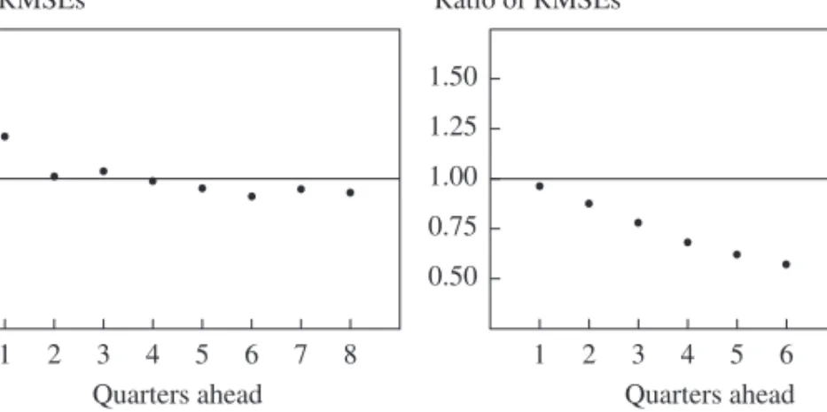
Figure 1. Relative Root Mean Square Errors of DSGE Model, BVAR,

and Greenbook Forecasts

Source: Authors’ calculations.

0.50 1.00 0.75 1.25 1.50 Ratio of RMSEs 1 2 3 4 5 6 7 8 Quarters ahead 0.50 1.00 0.75 1.25 1.50 Ratio of RMSEs 1 2 3 4 5 6 7 8 Quarters ahead

DSGE model relative to Greenbook Inflation

GDP growth

DSGE model relative to BVAR

DSGE model relative to Greenbook DSGE model relative to BVAR

0.50 1.00 0.75 1.25 1.50 Ratio of RMSEs 1 2 3 4 5 6 7 8 Quarters ahead 0.50 1.00 0.75 1.25 1.50 Ratio of RMSEs 1 2 3 4 5 6 7 8 Quarters ahead

In figure 1 we show results of this exercise with real-time data and com-pare the RMSEs of the DSGE model forecasts for inflation and GDP growth with those of the Greenbook and BVAR forecasts at different hori-zons. This figure, which reports the ratios of the RMSEs from two models, visually conveys a result that Smets and Wouters and Edge and others have shown earlier: except for inflation forecasts at very short horizons (where the Greenbook forecasts are better), the DSGE model forecasts have the lower RMSE for both inflation and growth in all comparisons. The litera-ture has taken this finding both as a vindication of the estimated medium-scale DSGE model, and as evidence that these models can be used for

forecasting as well as for positive analysis of counterfactuals and for informing optimal policy.

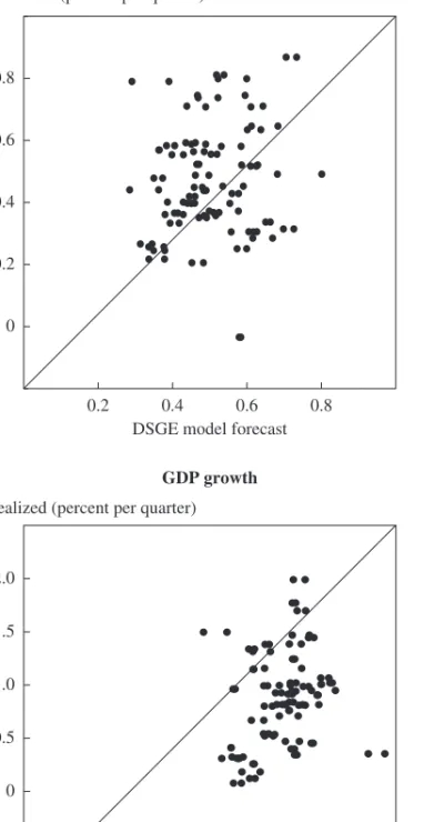
Although figure 1 does indeed show that the DSGE model has the best forecasting record among the three methods we consider, it offers no clues about how good the “best” is. To further evaluate the forecasts, we first present, in figure 2, scatterplots of the 4-quarter-ahead forecasts (a horizon at which the DSGE model outperforms the Greenbook and BVAR) of inflation and GDP growth from the DSGE model and the realized values of these variables. The better the forecast performance, the closer the obser-vations should fall to the 45-degree line.

Instead figure 2 shows that, for both variables, the points form clouds rather than 45-degree lines, suggesting that the 4-quarter-ahead forecast of the DSGE model is quite unrelated to the realized value. To get the full picture, we run a standard forecast efficiency test (see Gürkaynak and Wolfers 2007 for a discussion of tests of forecast efficiency and further ref-erences) and estimate the following equation:

A good forecast should have an intercept of zero, a slope coefficient of

1, and a high R2_{. If the intercept is different from zero, the forecast has on}

average been biased; if the slope differs from 1, the forecast has

consis-tently under- or overpredicted deviations from the mean, and if the R2_is

low, then little of the variation of the variable to be forecasted is captured

by the forecast. Note that especially when the point estimates of αh

yand βyh

are different from zero and 1, respectively, the R2_{is a more charitable}

mea-sure of the success of the forecast than the RMSE calculated in equation 1, as the errors in equation 2 are residuals obtained from the best-fitting line.

That is, a policymaker would make errors of size εh

y,tonly if she knew the

values of αh

yand βyhand used them to adjust ˆxyh. The R2that is comparable to

the RMSE measures calculated in equation 1 would be that implied by

equation 2 with αh

yand βyhconstrained to zero and 1, respectively.

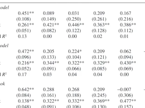
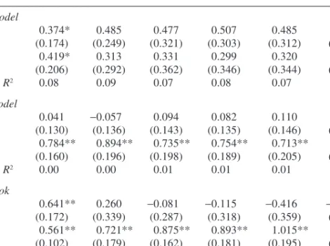
Tables 1, 2, and 3 show the estimation results of equation 2 for the DSGE model, BVAR, and Greenbook forecasts of inflation, GDP growth,

and interest rates.9_{The tables suggest that forecasts of inflation and GDP}

( )2 x_t h_y xˆ_{, ,}. y h y t h y t h =α +β +ε

9. The standard errors reported are Newey-West standard errors for 2h lags, given that there are two forecasts made in each quarter. Explicitly taking into account the clustering at the level of quarters (since forecasts made in the same quarter may be correlated) made no perceptible difference. Neither did using only the first or the second forecast in each quarter.

Figure 2. Realized and Four-Quarters-Ahead DSGE Forecast Inflation and GDP Growth

Source: Bureau of Economic Analysis data and authors’ calculations.

Realized (percent per quarter)

Realized (percent per quarter)

DSGE model forecast

Inflation 0 0.2 0.4 0.6 0.8 0.2 0.4 0.6 0.8

DSGE model forecast

GDP growth –0.5 0 0.5 1.0 1.5 2.0 –0.5 0 0.5 1.0 1.5

Table 1. Inflation Forecast Accuracy: DSGE, BVAR, and Greenbooka Quarters ahead Forecast 1 2 3 4 5 6 DSGE model Slope 0.451** 0.089 0.031 0.209 0.167 0.134 (0.108) (0.149) (0.250) (0.261) (0.216) (0.174) Intercept 0.261** 0.421** 0.446** 0.363** 0.386** 0.398** (0.051) (0.082) (0.122) (0.128) (0.112) (0.112) Adjusted R2 _{0.13 0.00 0.00 0.02 0.01 0.01} BVAR model Slope 0.472** 0.205 0.224* 0.209 0.062 −0.033 (0.096) (0.133) (0.104) (0.121) (0.094) (0.119) Intercept 0.216** 0.344** 0.322** 0.329** 0.430** 0.497** (0.052) (0.091) (0.066) (0.085) (0.069) (0.097) Adjusted R2 _{0.17 0.03 0.04 0.04 0.00 0.00} Greenbook Slope 0.642** 0.288 0.268 0.209 −0.007 −0.386 (0.084) (0.161) (0.188) (0.245) (0.306) (0.253) Intercept 0.138** 0.322** 0.332** 0.369** 0.477** 0.657** (0.048) (0.091) (0.106) (0.130) (0.157) (0.136) Adjusted R2 _{0.48 0.08 0.05 0.02 0.00 0.06}

Source: Authors’ regressions.

a. Sample size is 104 observations in all regressions. Standard errors are in parentheses. Asterisks indi-cate statistical significance at the **1 percent or the *5 percent level.

growth have been very poor by all methods, except for the Greenbook

inflation nowcast. The DSGE model inflation forecasts (table 1) have R2_s

of about zero for forecasts of the next quarter and beyond, and slope coef-ficients very far from unity. The DSGE model forecasts of GDP growth (table 2) likewise capture less than 10 percent of the actual variation in growth, and point estimates of the slopes are again far from unity. Again except for the Greenbook nowcast, the results are very similar for the Greenbook and the BVAR forecasts.

All three forecast methods, however, do impressively well at forecast-ing interest rates (table 3). This is surprisforecast-ing since short-term rates should be a function of inflation and GDP and thus should not be any more fore-castable than those two variables, except for the forecastability coming from interest rate smoothing by policymakers. The explanation here is that the interest rate is highly serially correlated, which makes it relative easy to forecast. (Indeed, in our sample the level of the interest rate behaves like a unit root process, as verified by an augmented Dickey-Fuller test not

reported here.)10_{Thus, table 3 may be showing long-run cointegrating}

rela-tionships rather than short-run forecasting ability. We therefore follow Gürkaynak, Brian Sack, and Eric Swanson (2005) in studying the change in the interest rate rather than its level.

Table 4 shows results for forecasts of changes in interest rates by the three methods. These results are now more comparable to those for the inflation and GDP growth forecasts, although in the short run there is higher forecastability in interest rate changes. The very strong nowcasting ability of the Greenbook derives partly from the fact that the Federal Reserve staff know that interest rate changes normally occur in multiples of 25 basis points, whereas, again, the BVAR and the DSGE model pro-duce continuous interest rate forecasts.

Table 2. GDP Growth Forecast Accuracy: DSGE, BVAR, and Greenbooka

Quarters ahead Forecast 1 2 3 4 5 6 DSGE model Slope 0.374* 0.485 0.477 0.507 0.485 0.553 (0.174) (0.249) (0.321) (0.303) (0.312) (0.279) Intercept 0.419* 0.313 0.331 0.299 0.320 0.284 (0.206) (0.292) (0.362) (0.346) (0.344) (0.311) Adjusted R2 _{0.08 0.09 0.07 0.08 0.07 0.06} BVAR model Slope 0.041 −0.057 0.094 0.082 0.110 0.037 (0.130) (0.136) (0.143) (0.135) (0.146) (0.206) Intercept 0.784** 0.894** 0.735** 0.754** 0.713** 0.815** (0.160) (0.196) (0.198) (0.189) (0.205) (0.263) Adjusted R2 _{0.00 0.00 0.01 0.01 0.01 0.00} Greenbook Slope 0.641** 0.260 −0.081 −0.115 −0.416 −0.001 (0.172) (0.339) (0.287) (0.318) (0.359) (0.422) Intercept 0.561** 0.721** 0.875** 0.893** 1.015** 0.852** (0.102) (0.179) (0.162) (0.181) (0.195) (0.233) Adjusted R2 _{0.13 0.01 0.00 0.00 0.02 0.00}

Source: Authors’ regressions.

a. Sample size is 104 observations in all regressions. Standard errors are in parentheses. Asterisks indi-cate statistical significance at the **1 percent or the *5 percent level.

10. Although nominal interest rates cannot theoretically be simple unit-root processes because of the zero nominal bound, they can be statistically indistinguishable from unit-root processes in small samples and pose the same econometric difficulties.

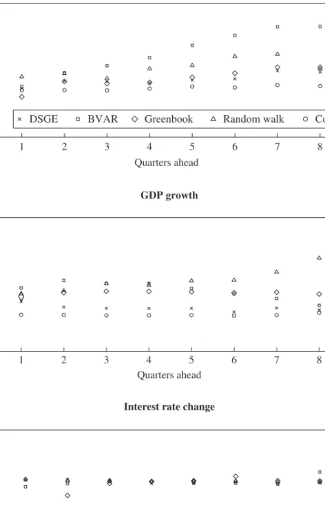
Taken together, figure 2 and tables 1 through 4 show that although the DSGE model forecasts are comparable to and often better than the Greenbook and BVAR forecasts, this is a comparison of very poor forecasts with each other. To provide a benchmark for forecast quality, we introduce a forecast series consisting simply of a constant and another that forecasts each variable as a random walk, and we ask the following two questions. First, if a policymaker could have used one of the above three forecasts over the 1992–2006 period, or could have had access to the actual mean of the series over the same period and used that as a forecast (using zero change as the interest rate forecast at all horizons), how would the RMSEs compare? Second, how large would the RMSEs be if the policymaker sim-ply used the last observation available on each date as the forecast for all

horizons, essentially treating the series to be forecast as random walks?11

Table 3. Interest Rate Forecast Accuracy: DSGE, BVAR, and Greenbooka

Quarters ahead Forecast 1 2 3 4 5 6 DSGE model Slope 1.138** 1.286** 1.373** 1.385** 1.381** 1.324* (0.031) (0.085) (0.181) (0.305) (0.416) (0.538) Intercept −0.149** −0.308** −0.427** −0.483 −0.528 −0.512 (0.027) (0.068) (0.153) (0.289) (0.422) (0.582) Adjusted R2 _{0.95 0.83 0.66 0.48 0.35 0.24} BVAR model Slope 0.924** 0.888** 0.867** 0.852** 0.828** 0.807** (0.020) (0.041) (0.076) (0.126) (0.191) (0.262) Intercept 0.056** 0.067 0.056 0.037 0.031 0.025 (0.020) (0.036) (0.064) (0.117) (0.195) (0.281) Adjusted R2 _{0.96 0.87 0.74 0.60 0.47 0.35} Greenbook Slope 0.993** 0.962** 0.904** 0.829** 0.735** 0.614** (0.006) (0.025) (0.057) (0.098) (0.148) (0.194) Intercept 0.001 0.012 0.049 0.112 0.200 0.316 (0.006) (0.025) (0.056) (0.096) (0.150) (0.205) Adjusted R2 _{1.00 0.96 0.87 0.72 0.54 0.36}

Source: Authors’ regressions.

a. Sample size is 104 observations in all regressions. Standard errors are in parentheses. Asterisks indi-cate statistical significance at the **1 percent or the *5 percent level.

11. In the random walk forecasts we set the interest rate change forecasts to zero. That is, in this exercise the assumed policymaker treats the level of the interest rate as a random walk.

The resulting RMSEs are depicted in figure 3. The constant forecast does about as well as the other forecasts, and often better, suggesting that the DSGE model, BVAR, and Greenbook forecasts do not contribute much information. It is some relief that the DSGE model forecast usually

does better than the random walk forecast, an often-used benchmark.12

However, the random walk RMSEs are very large. To put the numbers in perspective, observe that the RMSE of the 6-quarter-ahead inflation forecast of the DSGE model is about 0.22 in quarterly terms, or about

Table 4. Accuracy in Forecasting Changes in Interest Rates: DSGE, BVAR, and Greenbooka Quarters ahead Forecast 1 2 3 4 5 6 DSGE model Slope 0.498** 0.453* 0.560* 0.862* 1.127* 1.003 (0.121) (0.173) (0.240) (0.411) (0.473) (0.507) Intercept −0.012 −0.009 −0.017 −0.029 −0.041 −0.034 (0.016) (0.019) (0.023) (0.028) (0.031) (0.031) Adjusted R2 _{0.15 0.11 0.11 0.17 0.20 0.12} BVAR model Slope 0.724** 0.978** 1.202* 1.064* 1.025* 1.040* (0.133) (0.274) (0.459) (0.489) (0.476) (0.482) Intercept −0.018 −0.027 −0.044 −0.043 −0.040 −0.038 (0.014) (0.019) (0.028) (0.033) (0.033) (0.033) Adjusted R2 _{0.30 0.17 0.16 0.16 0.17 0.18} Greenbook Slope 1.052** 1.191** 0.986** 0.588 0.423 −0.279 (0.030) (0.144) (0.212) (0.358) (0.215) (0.333) Intercept −0.006 −0.022 −0.023 −0.011 −0.006 0.005 (0.003) (0.013) (0.022) (0.023) (0.024) (0.022) Adjusted R2 _{0.96 0.50 0.14 0.03 0.02 0.01}

Source: Authors’ regressions.

a. Sample size is 104 observations in all regressions. Standard errors are in parentheses. Asterisks indi-cate statistical significance at the **1 percent or the *5 percent level.

12. We also looked at how the DSGE model forecast RMSEs compare statistically with other forecast RMSEs (results available from the authors upon request). Results of Diebold-Mariano tests show that for inflation, the RMSE of the DSGE model is significantly lower than those of the BVAR and the random walk forecasts for most maturities, is indistinguish-able from the RMSE of the Greenbook, and is higher than that of the constant forecast for some maturities; for GDP growth the DSGE model RMSE is statistically lower than those of the BVAR and the random walk forecasts and is indistinguishable from the RMSEs of the Greenbook and the constant forecasts.

Figure 3. Root Mean Square Errors of Alternative Forecasts

Source: Authors’ calculations.

RMSE Quarters ahead Inflation 0.1 0.2 0.3 0.4 2 3 1 4 5 6 7 8 GDP growth

Interest rate change

RMSE Quarters ahead 0.4 0.6 0.8 1.0 2 3 1 4 5 6 7 8 RMSE Quarters ahead 0 0.05 0.10 0.15 2 3 1 4 5 6 7 8

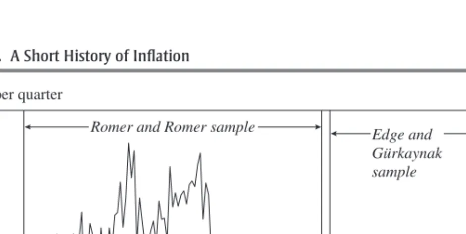
Figure 4. A Short History of Inflation

Source: BEA data.

Edge and Gürkaynak sample Romer and Romer sample

1965 0.5 1.0 1.5 2.0 2.5 3.0

Percent per quarter

1970 1975 1980 1985 1990 1995 2000 2005

0.9 percent annualized, with a 95 percent confidence interval that is 3.6 percentage points wide. That is not very useful for policymaking.

IV. Discussion

Our findings, especially those for inflation, are surprising given the finding of Christina Romer and David Romer (2000) that the Greenbook is an excellent forecaster of inflation at horizons out to 8 quarters. Figure 4 shows the reason for the difference between their finding and ours. The Romer and Romer sample covers a period when inflation swung widely, whereas our sample—and the sample used in other studies for DSGE model forecast evaluations—covers a period when inflation behaved more like independent and identically distributed (i.i.d.) deviations around a constant. That is, there is little to be forecasted over our sample.

This finding is in line with Stock and Watson’s (2007) result that after the Great Moderation began, the permanent (forecastable) component of inflation, which had earlier dominated, diminished in importance, and the bulk of the variance of inflation began to be driven by the transitory (unforecastable) component. It is therefore not surprising that no forecast-ing method does well. Bharat Trehan (2010) shows that a similar lack of forecastability is also evident in the Survey of Professional Forecasters (SPF) and the University of Michigan survey of inflation expectations. Andrew Atkeson and Lee Ohanian (2001) document that over the period 1984 to 1999, a random walk forecast of 4-quarter-ahead inflation

out-performs the Greenbook forecast as well as Phillips curve models. (But our analysis finds that the DSGE model, with a sophisticated, microfounded Phillips curve, outperforms the random walk forecast.) Jeff Fuhrer, Giovanni Olivei, and Geoffrey Tootell (2009) show that this is due to the parameter changes in the inflation process that occurred with the onset of the Great Moderation. For forecasts of output growth, Tulip (2009) docu-ments a notably larger reduction in actual output growth volatility follow-ing the Great Moderation relative to the reduction in Greenbook RMSEs, thus indicating that much of the reduction in output growth volatility has stemmed from the predictable component—the part that can potentially be forecast.

David Reifschneider and Tulip (2007) perform a wide-reaching analy-sis of institutional forecasts—those of the Greenbook, the SPF, and the Blue Chip, as well as forecasts produced by the Congressional Budget Office and the administration—for real GDP (or GNP) growth, the unemployment rate, and consumer price inflation. Although they do not consider changes in forecast performance associated with the Great Moderation, their analysis, which is undertaken for the post-1986 period, finds overwhelmingly that errors for all institutional forecasts are large. More broadly, Antonello D’Agostino, Domenico Giannone, and Paolo Surico (2006) also consider a range of time-series forecasting models, including univariate AR models, factor-augmented AR models, and pooled bivariate forecasting models, as well as institutional forecasts— those of the Greenbook and the SPF—and document that although RMSEs for forecasts of real activity, inflation, and interest rates dropped notably with the Great Moderation, time-series and institutional forecasts also largely lost their ability to improve on a random walk. Jon Faust and Jonathan Wright (2009) similarly note that the performance of some of the forecasting methods they consider improves when data from periods pre-ceding the Great Moderation are included in the sample.

We would argue that DSGE models should not be judged solely by their absolute forecasting ability or lack thereof. Previous authors, such as Edge and others (2010), were conscious of the declining performance of Greenbook and time-series forecasts when they performed their compari-son exercises but took as given the fact that staff at the Federal Reserve Board are required to produce Greenbook forecasts of the macroeconomy eight times a year. More precisely, they asked whether a DSGE model forecast should be introduced into the mix of inputs used to arrive at the final Greenbook forecast. In this case relative forecast performance is a relevant point of comparison. Another noteworthy aspect of central bank

13. The divine coincidence (see Blanchard and Galí 2007 for the first use of this term in print) refers to a property of New Keynesian models in which stabilizing inflation is equiva-lent to stabilizing the output gap, defined as the gap between actual output and the natural rate of output.

14. However, see Galí (2010) about the difficulties inherent in generating counterfactual scenarios using DSGE models.

forecasting is that of “storytelling”: not only are the values of the forecast variables important, but so, too, is the narrative explaining how present imbalances will be unwound as the macroeconomy moves toward the bal-anced growth path. A well-thought-out and much-scrutinized story accom-panies the Greenbook forecast but is not something present in reduced-form time-series forecasts. An internally consistent and coherent narrative is, however, implicit in a DSGE model forecast, indicating that these models can also contribute along this important dimension of forecasting.

In sum, what do these findings say about the quality of DSGE models as a tool for telling internally consistent, reasonable stories for counter-factual scenarios? Not much. That inflation will be unforecastable is a prediction of basic sticky-price DSGE models when monetary policy responds aggressively to inflation. Marvin Goodfriend and Robert King (2009) make this point explicitly using a tractable model. If inflation is forecasted to be high, policymakers will increase interest rates and attempt to rein in inflation. If they are successful, inflation will never be predictably different from the (implicit) target, and all of the variation will come from unforecastable shocks. In models lacking real rigidities,

the “divine coincidence” will be present,13_{which means that the output}

gap will have the same property of unforecastability. Thus, it is quite pos-sible that the model is “correct” and therefore cannot forecast cyclical fluctuations but that the counterfactual scenarios produced by the model

can still inform policy discussions.14

Of course, the particular DSGE model we employ in this paper does not have the divine coincidence, because of the real rigidities it includes, such as a rigidity of real wages due to having both sticky prices and sticky wages. Moreover, because this model incorporates a trade-off between stabilizing price inflation, wage inflation, and the output gap, optimal pol-icy is not characterized by price inflation stabilization, and therefore price inflation is not unforecastable. Nonetheless, price inflation stabilization is a possible policy, which could be pursued even if not optimal, and this would imply unforecastable inflation. That said, this policy would likely not stabilize the output gap, thus implying some forecastability of the out-put gap. Ultimately, whether and to what extent the model implies

fore-castable or unforefore-castable fluctuations in inflation and GDP growth can be learned by simulating data from the model calibrated under different monetary policy rules and performing forecast exercises on the simulated data. We note the qualitative implication of the model that there should not be much predictability, especially for inflation, and leave the quanti-tative study to future research. Note also that our discussion here has focused on the forecastability of the output gap, not of output growth, which is ultimately the variable of interest in our forecast exercises. Unforecastability of the output gap need not imply unforecastability of output growth.

Finally, we would note that a reduced-form model with an assumed inflation process that is equal to a constant with i.i.d. deviations—in other words, a “wrong” model—will also have the same unforecastability impli-cation. Thus, evaluating forecasting ability during a period such as the Great Moderation, when no method is able to forecast, is not a test of the empirical relevance of a model.

V. Robustness and Extensions

To verify that our results are not specific to the relatively short sample we have used or to the Greenbook vintages we employed, we repeated the exercise using Blue Chip forecasts as the judgmental forecast for the 1992–2010 period. (This test also has the advantage of adding the financial crisis and the Great Recession to our sample.) For this exercise we esti-mated the DSGE model and the BVAR using data vintages of Blue Chip publication dates and produced forecasts.

For the sake of brevity, we do not show the analogues of the earlier fig-ures and tables but simply note that the findings are very similar when Blue Chip forecasts replace Greenbook forecasts and the sample is extended to 2010. (One difference is that the Blue Chip forecast has nowcasting ability for GDP as well as inflation.) The DSGE model forecast is similar to the judgmental forecast and is better than the BVAR, in terms of RMSEs, at almost all horizons, but all three forecasts are again very poor. (This exer-cise omits the forecasts of interest rates, since the Blue Chip forecasts do not include forecasts of the overnight rate.) The longer sample allows us to answer some interesting questions and provide further robustness checks.

Although we again use quarter-over-quarter changes and not annual growth rates for all of our variables, overlapping periods in long-horizon forecasting are a potential issue. In figure 5 we show the nonoverlapping, 4-quarter-ahead absolute errors of DSGE model forecasts made in January

of each year for the first quarter of the subsequent year. The horizontal

lines at −0.25 and 0.25 indicate forecast errors that would be 1 percentage

point in annualized terms. Most errors are near or outside these bounds. It is thus clear that our statistical results are not driven by outliers (a fact also visible in figure 2).

To provide a better understanding of the evolution of forecast errors over time, figure 6 shows 3-year rolling averages of RMSEs for 4-quarter-ahead forecasts, using all 12 forecasts for each year. Not surprisingly, these average forecast errors are considerably higher in the latter part of the sample, which includes the crisis episode. The DSGE model does

Figure 5. Nonoverlapping DSGE Four-Quarters-Ahead Forecast Errorsa

Source: Authors’ calculations.

a. Horizontal lines at 0.25 and –0.25 indicate thresholds for errors exceeding 1 percentage point annualized. Inflation –0.50 –0.25 0 0.25 0.50

Percent per quarter

Percent per quarter

GDP growth 1994 1996 1998 2000 2002 2004 2006 2008 –2 –1 0 1 2 1994 1996 1998 2000 2002 2004 2006 2008

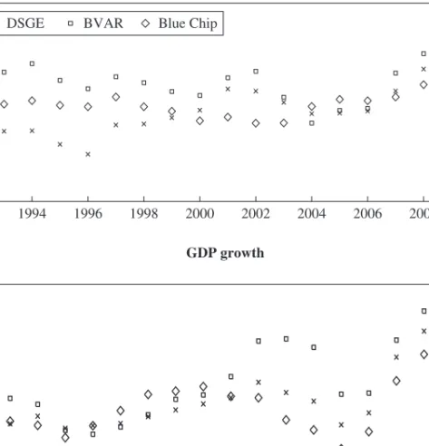
Figure 6. Three-Year Rolling Averages of Four-Quarters-Ahead RMSEs

DSGE BVAR Blue Chip

Source: Authors’ calculations.

RMSE Inflation 0.1 0.2 0.3 0.4 GDP growth RMSE 0.25 0.50 0.75 1.00 1.25 1994 1996 1998 2000 2002 2004 2006 2008 1994 1996 1998 2000 2002 2004 2006 2008

worse than the Blue Chip forecast once the rolling window includes 2008, for both the inflation and the GDP growth forecasts.

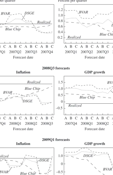
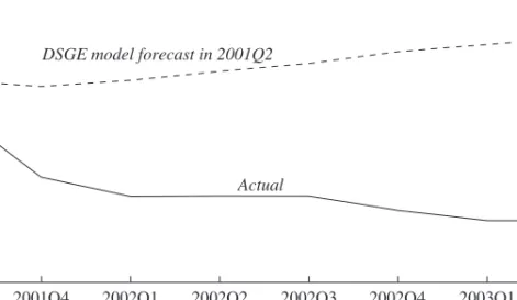
Lastly, we compare the forecasting performance of the DSGE and BVAR models with that of the Blue Chip forecasts during the recent crisis and recession. Figure 7 shows the forecast errors beginning with 4-quarter-ahead forecasts and ending with the nowcast for three quarters: 2007Q4, the first quarter of the recession according to the National Bureau of Economic Research dating; 2008Q3, when Lehman Brothers failed and growth in GDP per capita turned negative; and 2009Q1, when the extent of the contraction became clear (see Wieland and Wolters

Figure 7. Forecasts of Inflation and GDP Growth during the 2007–08 Crisis 0.2 0.6 0.4 0.8 1.0

Percent per quarter

Forecast date 2007Q4 forecasts 2008Q3 forecasts 2009Q1 forecasts Inflation Inflation Inflation A B C A B C A B C A B C 2007Q1 2007Q2 2007Q3 2007Q4 BVAR Blue Chip Realized DSGE 0.2 0.6 0.4 0.8 1.0 Forecast date A B C A B C A B C A B C 2007Q4 2008Q1 2008Q2 2008Q3 BVAR Blue Chip Realized DSGE 0 0.4 0.2 0.6 0.8 Forecast date A B C A B C A B C A B C 2008Q2 2008Q3 2008Q4 2009Q1

BVAR _{Blue Chip}

Realized

DSGE

Percent per quarter

GDP growth 0.2 0.6 0.4 0.8 1.0 1.2 Forecast date GDP growth GDP growth A B C A B C A B C A B C 2007Q1 2007Q2 2007Q3 2007Q4 BVAR Blue Chip Realized DSGE –0.5 0.5 0 1.0 1.5 Forecast date A B C A B C A B C A B C 2007Q4 2008Q1 2008Q2 2008Q3 BVAR Blue Chip Realized DSGE –1.0 0 –0.5 1.0 Forecast date A B C A B C A B C A B C 2008Q2 2008Q3 2008Q4 2009Q1 BVAR Blue Chip Realized DSGE

2010 for a similar analysis of more episodes). In all six panels in figure 7, the model forecast and the judgmental forecast are close to each other when the forecast horizon is 4 quarters. Although all the forecasts clearly first miss the recession, and then miss its severity, the Blue Chip forecasts in general fare better as the quarter to be forecasted gets closer, and especially when nowcasting.

An interesting point is that the judgmental forecast improves within quarters, especially the nowcast quarter, whereas the DSGE and BVAR model forecasts do not. As the quarter progresses, the DSGE model and the BVAR model have access only to more revised versions of data pertaining to previous quarters. Forecasters surveyed by the Blue Chip sur-vey, however, observe within-quarter information such as monthly fre-quency data on key components of GDP and GDP prices as well as news about policy developments. Also, the Blue Chip forecasters surely knew of the zero nominal bound, whereas both of the estimated models (DSGE and BVAR) imply deeply negative nominal rate forecasts during the crisis.

It is not very surprising that judgmental forecasts fare better in captur-ing such regime switches. The DSGE model, lackcaptur-ing a financial sector and a zero nominal bound on interest rates, should naturally do somewhat bet-ter in the precrisis period. In fact, that is the period this model was built to explain. But this also cautions us that out-of-sample tests for DSGE models are not truly out of sample as long as the sample is in the period the model was built to explain. The next generation of DSGE models will likely include a zero nominal bound and a financial sector as standard features and will do better when explaining the Great Recession. Their real test will be to explain—but not necessarily to forecast—the first business

cycle that follows those models’ creation.15

VI. Conclusion

DSGE models are very poor at forecasting, but so are all other approaches. Forecasting ability is a nonissue in DSGE model evaluation, however, because in recent samples (over which these models can be evaluated using real-time data) there is little to be forecasted. This is consistent with

15. A promising avenue of research is adding unemployment explicitly to the model, as in Galí, Smets, and Wouters (2010). This will likely help improve the model forecasts, as Stock and Watson (2010) show that utilizing an unemployment gap measure helps improve forecasts of inflation in recession episodes.

the literature on the Great Moderation, which emphasizes that not only the standard deviation of macroeconomic fluctuations but also their nature has changed. In particular, cycles today are driven more by temporary, unfore-castable shocks.

The lack of forecasting ability is not, however, evidence against the DSGE model. Forecasting ability is simply not a proper metric by which to judge a model. Indeed, the DSGE model’s poor recent forecasting record can be evidence in favor of it. Monetary policy was characterized by a strongly stabilizing rule in this period, and the model implies that such pol-icy will undo predictable fluctuations, especially in inflation. We leave fur-ther analysis of this point and of the forecasting ability of the model in pre-and post–Great Moderation periods to future work.

A P P E N D I X

Constructing the Real-Time Datasets

In this appendix we discuss how we constructed the real-time datasets that we use to generate all of the forecasts other than those of the Greenbook. To ensure that when we carry out our forecast performance exercises we are indeed comparing the forecasting ability of different methodologies (and not some other difference), it is critical that the datasets and other information that we use to generate our model forecasts are the same as those that were available when the Greenbook and Blue Chip forecasts were generated. For this we are very conscious of the timing of the releases of the data that we use to generate our model forecasts and how they relate to the Greenbook’s closing dates and Blue Chip publication dates.

We begin by documenting the data series used in the DSGE model and in the other reduced-form forecasting models. Here relatively little discus-sion is necessary, since we employ essentially all of the same data series used by Smets and Wouters in estimating their model. We then move on to provide a full account of how we constructed the real-time datasets used to generate the model forecasts. We then briefly explain our construction of the “first final” data, which are ultimately what we consider to be the real-ized values of real GDP growth and the rate of GDP price inflation against which we compare the forecasts.

Data Series Used

To allow comparability with the results of Smets and Wouters (2007), we use exactly the same data series that they used in their analysis.

Because we will subsequently have to obtain different release vintages for all of our data series (other than the federal funds rate), we need to be very specific about not only which government statistical agency is the source of the data series but also which data release we use.

Four series used in our estimation are taken from the national income and product accounts (NIPA). These accounts are produced by the Bureau of Economic Analysis and are constructed at quarterly frequency. The four series are real GDP (GDPC), the GDP price deflator (GDPDEF), nominal personal consumption expenditures (PCEC), and nominal fixed private investment (FPI). The variable names that we use, except that for real GDP, are also the same as those used by Smets and Wouters. We use a dif-ferent name for real GDP because whereas Smets and Wouters define real GDP in terms of chained 1996 dollars, in our analysis the chained dollars for which real GDP is defined change with the data’s base year. (In fact, the GDP price deflator also changes with the base year, since it is usually set to 100 in the base year.)

Another series used in our estimation is compensation per hour in the nonfarm business sector (PRS85006103), taken from the Bureau of Labor Statistics’ quarterly Labor Productivity and Costs (LPC) release. The vari-able name is that assigned to it by the data service (Macrospect) that Smets and Wouters used to extract their data.

Three additional series used in our estimation are taken from the Employment Situation Summary (ESS), which contains the findings of two surveys: the Household Survey and the Establishment Survey. These three series, which are produced by the Bureau of Labor Statistics and con-structed at monthly frequency, are average weekly hours of production and nonsupervisory employees for total private industries (PRS85006023), civilian employment (CE16OV), and civilian noninstitutional population (LNSINDEX). The first of these series is from the Establishment Survey and the other two are from the Household Survey. Since our model is quar-terly, we calculate simple quarterly averages of the monthly data.

The final series in our model, the federal funds rate, differs from the others in that it is not revised after the first release. This series is obtained from the Federal Reserve Board’s H.15 release, published every business day, and our quarterly series is simply the averages of these daily data.

We transform all of our data sources for use in the model in exactly the same way as Smets and Wouters:

consumption = ln[(PCEC/GDPDEF)/LNSINDEX] × 100

output = ln(GDPC/LNSINDEX) × 100

hours = ln[(PRS85006023 × CE16OV/100)/LNSINDEX] × 100

inflation = ln(GDPDEF/GDPDEF₋₁) × 100

real wage = ln(PRS85006103/GDPDEF) × 100

interest rate = federal funds rate ÷ 4.

Obtaining the Real-Time Datasets Corresponding to Greenbook Forecasts

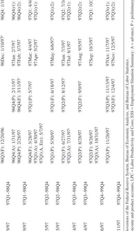
Appendix table A1 provides for the year 1997 what, in the vertical dimension, is essentially a timeline of the dates of all Greenbook forecasts and all release dates for the data sources that we use and that revise. The horizontal dimension of the table sorts the release dates by data source. The online appendix includes a set of tables for the whole 1992–2004 sam-ple period. From these tables it is reasonably straightforward to understand how we go about constructing the real-time datasets that we use to estimate the models from which we obtain our model forecasts to be compared with the Greenbook forecasts. Specifically, for each Greenbook forecast the table shows the most recent release, or vintage, of each data source at the time that edition of the Greenbook closed. For example, for the June 1997 Greenbook forecast, which closed on June 25, the tables show that the most recent release of NIPA data was the preliminary release of 1997Q1, on May 30, and the most recent release of the LPC data was the final

release of 1997Q1, on June 18.16

The ESS data require a little more explanation. These are monthly series for which the first estimate of the data is available quite promptly (within a week) after the data’s reference period. Thus, for example, the last release of the ESS before the June 1997 Greenbook is that for May 1997, released on June 6. Each ESS release, however, includes not only the first estimate of the preceding month’s data (in this case May) but also revisions to the two preceding months (in this case April and March). This means that from the perspective of thinking about quarterly data, the June 6

ESS release represents the second and final revision of 1997Q1 data.17

16. Until last year the three releases in the NIPA were called the advance release, the preliminary release, and the final release. Thus, the preliminary release described above is actually the second of the three. Last year, however, the names of the releases were changed to the first release, the second release, and the final release. We refer to the original names of the releases in this paper. Note also that there are only two releases of the LPC for each quar-ter. These are called the preliminary release and the final release.

17. Of course, the release also contains two-thirds of the data for 1997Q2, but we do not use this information at all. This is reasonably standard practice.

Table A1.

Dates of Greenbook Forecasts and NIPA, LPC, and ESS Releases, 1997

a Greenbook Greenbook Interim NIPA Interim LPC Interim ESS Interim ESS Month closed forecast horizon releases releases releases (monthly) releases (quarterly) 96Q3(F): 12/20/96 96Dec: 1/10/97 b 96Q4: 1/10/97 January † 1/29/97 97Q1–98Q4 96Q4(A): 1/31/97 96Q4(P): 2/11/97 97Jan: 2/7/97 96Q4(r1): 2/7/97 96Q4(P): 2/28/97 96Q4(F): 3/11/97 c 97Feb: 3/7/97 96Q4(r2): 3/7/97 March 3/19/97 97Q1–98Q4 96Q4(F): 3/28/97 97Q1(P): 5/7/97 97Mar: 4/4/97 97Q1: 4/4/97 97Q1(A): 4/30/97 97Apr: 5/2/97 97Q1(r1): 5/2/97 97Q1(A, Err): 5/7/97 May 5/15/97 97Q2–98Q4 97Q1(P): 5/30/97 97Q1(F): 6/18/97 97May: 6/6/97 d 97Q1(r2): 6/6/97 June 6/25/97 97Q2–98Q4 97Q1(F): 6/27/97 97Q2(P): 8/12/97 e 97Jun: 7/3/97 97Q2: 7/3/97 97Q2(A): 7/31/97 c 97Jul: 8/1/97 97Q2(r1): 8/1/97 August 8/14/97 97Q3–98Q4 97Q2(P): 8/28/97 97Q2(F): 9/9/97 97Aug: 9/5/97 97Q2(r2): 9/5/97 September 9/24/97 97Q3–99Q4 97Q2(F): 9/26/97 97Sep: 10/3/97 97Q3: 10/3/97 97Q3(A): 10/31/97 November 11/6/97 97Q4–99Q4 97Q3(P): 11/26/97 97Q3(P): 11/13/97 97Oct: 11/7/97 97Q3(r1): 11/7/97 97Q3(F): 12/4/97 97Nov: 12/5/97 97Q3(r2): 12/5/97 December 12/11/97 97Q4–99Q4

Sources: Board of Governors of the Federal Reserve System, Bureau of Economic Analysis, and Bureau of Labor Statistics. a. NIPA

=

national income and product accounts; LPC

=

Labor Productivity and Costs; ESS

=

Employment Situation Summary; A

= advance; P = preliminary; F = final; Err =

corrected; r1 and r2, first and second revisions. Dagger indicates rounds for which one more quarter of employment data than of

NIPA data are available.

By looking up what vintage of the data was available at the time of each Greenbook, we can construct a dataset corresponding to each Greenbook that contains observations for each of our model variables taken from the correct release vintage. All vintages for 1992 to 1996 (shown in tables 1 to 5 in the online appendix) were obtained from ALFRED, an archive of Federal Reserve economic data maintained by the St. Louis Federal Reserve Bank. All vintages for 1997 to 2004 (shown in tables 6 to 13 in the online appendix and, for 1997, in table A1 in this paper) were obtained from datasets that since September 1996 have been archived by Federal Reserve Board staff at the end of each Greenbook round.

In the June 1997 example given above, the last observation that we have for each data series is the same: 1997Q1. This will not always be the case. For example, in every January Greenbook round, LPC data are not avail-able for the preceding year’s fourth quarter, ESS data are always availavail-able, and NIPA data are sometimes available, specifically, only in the years 1992–94. This means that in the January Greenbook for all years other than 1992–94, there is one more quarter of employment data than of NIPA data. This is also the case in the October 2002 and 2003 Greenbooks; all Greenbooks for which this is an issue are marked with a dagger (†) in table A1 of this paper and in tables 1 to 13 of the online appendix.

Differences in data availability can also work the other way. For exam-ple, in the Greenbooks marked with an asterisk (*) in table A1 of this paper and tables 1 to 13 of the online appendix, there is always one less observa-tion of the LPC data than of the NIPA data. We use the availability of the NIPA data as what determines whether data are available for a given quar-ter or not. Thus, if we have an extra quarquar-ter of ESS data (as we do in the rounds indicated by †), we ignore those data, even those for HOURS, in making our first quarter-ahead forecasts. If instead we have one less quar-ter of the LPC data (as we do in the rounds indicated by *), we use the Federal Reserve Board staff’s estimate of compensation per hour for the quarter, which is calculated based on the ESS’s reading of average hourly earnings. This is always available in real time, since the ESS is very prompt. Of course, this raises the question of why (given its timeliness) we do not just use the ESS’s estimate for wages (that is, average hourly earn-ings for total private industry) instead of the LPC’s compensation per hour for the nonfarm business sector series. One reason is our desire to stay as close as possible to Smets and Wouters, but another is that real-time data on average hourly earnings in ALFRED extend back only to 1999. Also, there are much more elegant ways to deal with the lack of uniformity in data availability that we face. In particular, the Kalman filter, which is