Comparison Of Different Covariance Structure Used For Experimental Design With Repeated Measurement

Comparison of different covariance structure

used for experimental design with repeated

measurement

ARTICLE in JOURNAL OF ANIMAL AND PLANT SCIENCES Impact Factor: 0.55 CITATIONS

2

DOWNLOADS

53

VIEWS

91

2 AUTHORS: Ecevit Eyduran Iğdır Üniversitesi 50 PUBLICATIONS 52 CITATIONS SEE PROFILE Yavuz Akbas Ege University 34 PUBLICATIONS 166 CITATIONS SEE PROFILE

COMPARISON OF DIFFERENT COVARIANCE STRUCTURE USED FOR

EXPERIMENTAL DESIGN WITH REPEATED MEASUREMENT

E. Eyduran and Y. Akbaş*

Iğdır University, Faculty of Agriculture, Department of Animal Science, 76000, Iğdır, Turkey *Ege University, Faculty of Agriculture, Department of Animal Science, Bornova-İzmir, Turkey

Crossponding author e-mail:ecevit.eyduran@gmail.com

ABSTRACT

This study was conducted to compare performance of univariate and multivariate approaches used for analyzing experiments with repeated measurement and determine the best covariance structure for the data studied. In this study, univariate ANOVA, Geisser-Greenhouse Epsilon and Huynth-Feldt Epsilon were used as univariate approaches while profile analysis, Containment, Satterthwaite and Kenward-Roger approaches in general linear mixed model were applied as multivariate approaches. Annual amounts of wheat production from 65 provinces in seven geographical regions of Turkey from 1982 to 1999 were used as research material. A total of 1170 production values were obtained. In General Linear Model, nine various covariance structures (CS, CSH, UN, HF, AR (1), ARH (1), ANTE (1), TOEP and TOEPH) were applied. AIC and AICC criteria were used to determine the most appropriate covariance pattern for fitting data. In the study, “spherity assumption” for amounts of wheat production of provinces was violated. Application of Containment, Satterthwaite and Kenward-Roger approaches in general linear model and determination of covariance structure with the best fit were provided. According to AIC and AICC fitting criteria, it was determined that CS covariance structure gave the best fit to data set. As a result, covariance structure is compound symmetry (CS) in standard univariate ANOVA, and unstructured (UN) covariance structure in MANOVA. However, determination of the most appropriate covariance structure for data set is possible in multivariate general linear model. Containment, Satterthwaite, and Kenward-Roger approaches gave similar results since total sample size was sufficient. On the other hand, usage of Containment, Satterthwaite and Kenward-Roger approaches in analyzing experiments with repeated measurement were suggested to allow selection of the most suitable covariance structure for data set.

Key Words: Repeated Measurements, Repeated ANOVA, Profile Analysis, General Linear Model, Containment, Kenward Roger, Satterthwaite.

INTRODUCTION

Repeated measures are multiple responses taken in sequential from same experimental unit over time. The best example to this type data (trait-time) in animal science is “Growth Curve” data, describing growth at certain time period of each experimental unit (Akbaş et al., 2001).

The repeated measurement designs with one between-subject (treatment) and within-subject (time) factors are used commonly in medicine, psychology and education. Experimental designs with this repeated measurement are similar to split-plot experiment design that has treatment and time as two factors (Littell et al., 1998). Besides, the experimental designs in literature have been also called within-subject design or correlated groups design (Kowachuk, 2000; Gürbüz et al., 2003).

Univariate and multivariate analysis approaches have been used for analyzing repeated measures data including between-subject and within-subject factors. Univariate approaches are “Repeated ANOVA”, This paper is a part of Ph.D thesis of first author.

“Greenhouse-Geisser Epsilon (G-G) adjusted F test” and “Huynh-Feldt Epsilon (H-F) adjusted F test”. In “Repeated ANOVA”, Spherity assumption should be provided. When this assumption is violated, repeated measurement design is analyzed using “Greenhouse-Geisser Epsilon (G-G) adjusted F test”, and “Huynh-Feldt Epsilon (H-F) adjusted F test” or multivariate approaches. Multivariate approaches for repeated measures designs are “Profile Analysis” and “Mixed model methodology”. In case of violation of the assumption, it was reported that multivariate approaches was more superior to univariate approaches (Huynh and Feldt, 1970; Olson, 1974; Barcikowski and Robey, 1984; Looney and Stanley, 1989; Keselman et al., 1993; Algina and Oshima, 1994; Tabachnichk and Fidel, 2001; Gürbüz et al., 2003; Eyduran et al., 2008). Contrary to “Repeated ANOVA”, “Greenhouse-Geisser Epsilon (G-G) adjusted F test”, “Huynh-Feldt Epsilon (H-F) adjusted F test” and Profile analysis approaches, mixed model methodology allows us to directly select different covariance structures for repeated measures design with/without missing data. When even one measure of an experimental unit (animal) in univariate and Profile Analysis approaches is missing,

all data of the experimental unit are ignored. On the other hand, when there are several missing data of an experimental unit in mixed model methodology, all data of the unit do not need to be deleted.

In repeated measures design, approaches used with covariance structures available in mixed model methodology are Containment, Satterthwaite and Kenward Roger. In literature, there were very few studies on comparison of these three approaches with alternative covariance structures in general linear (mixed) model.

The first aim of this study was to compare performance of univariate and multivariate approaches used for analyzing repeated measures data with between-subject and within-between-subject factors. The second aim was to

determine the suitable covariance structure for repeated measurements.

MATERIALS AND METHODS

As material in this study, annual amounts of wheat production belonging to 65 provinces in seven geographical regions of Turkey from 1982 to 1999 were used (TUİK, 1982; TUİK 1999). A total of 1170 production values were taken from these provinces. During this time period, provinces not having data for some years were not included. In the preliminary analysis, it was determined that wheat production was not followed normal distribution and data were transformed to Log10.

Table1. Distribution of provinces according to regions used in the study Central

Anatolia

Mediterranean Sea

Aegean Marmara BlackSea Southeast Anatolia

Eastern Anatolia

Ankara Adana Afyon Balıkesir Amasya Adıyaman Ağrı

Çankırı Antalya Aydın Bilecik Artvin Diyarbakır Bingöl

Eskişehir Burdur Denizli Bursa Bolu Gaziantep Bitlis

Kayseri Hatay İzmir Çanakkale Çorum Mardin Elazığ

Kırşehir Isparta Kütahya Edirne Giresun Siirt Erzincan

Konya İçel Manisa İstanbul Gümüşhane Şanlıurfa Erzurum

Nevşehir Maraş Muğla Kırklareli Kastamonu Hakkâri

Niğde Uşak Kocaeli Ordu Kars

Sivas Sakarya Samsun Malatya

Yozgat Tekirdağ Sinop Muş

Tokat Tunceli

Zonguldak Van

In addition, “multivariate normal distribution” assumption was provided for data set studied (Alpar, 2003).

In this study, “geographical region” (treatment) was independent factor while “year” (time) was repeated factor. The repeated measures design in the study has one between-subject (treatment) and one within-subject (time) factors. Number of levels of “geographical region” and “year” factors are seven and eighteen, respectively. Provinces in each geographical region are thought as experimental unit. The model can be written as:

 

( ) ijk j k jk i j ijk Y        e (1) (i=1,2,...,k ; j=1,2,...,p and m=1,2,...,ni ) Where;  : grand mean

j : effect of j th level of “geographical region”

factor ( ) i j



: the random effect of ith _province

(experimental unit) in jth _{geographical region}

k : kth year effect,

jk: effect of geographical region by year

interaction,

eijk : randor error term.

However, in the current study,



i j( ) _{was not included in} the model

Other effects except eijk are fixed effects.

Seven approaches used in the study are given below:

 Univariate approaches

1. Repeated ANOVA (Split-Plot design)

2. Greenhouse-Geisser Epsilon (G-G) adjusted F test approach

3. Huynh-Feldt Epsilon (H-F) adjusted F test approach  Multivariate Approaches

4. Profile Analysis Approach

5. Containment as an adjusted df approach in General Linear Model

6. Satterthwaite as an adjusted df approach in General Linear Model

7. Kenward-Roger as an adjusted df approach in General Linear Model

Generally, Greenhouse-Geisser Epsilon (G-G) and Huynh-Feldt Epsilon (H-F) adjusted F test approaches are traditionally used when spherity assumption is violated (Keskin and Mendeş, 2001). The sphericity assumption is an assumption about the structure of the covariance matrix in a repeated measures design. Sphericity relates to the equality of the variances of the differences between data taken from same unit. Mauchly's sphericity test controls the hypothesis that the variances of the differences between groups are equal as :

1) (p ) (tr 1) (p 1) (p W _    CSC' C' S C (2) Where;

S: estimation of covariance matrix from sample

C: orthonormal matrix that include independent contrasts among (p-1) number means with dimension (p-1) x p.

Approximate distribution of W statistic is chi-square with df [p(p-1)/2]-1. The statistic can be calculated as: lnW 1) 6(p 3 3p 2p v χ 2 2               (3)

Mauchly's sphericity test is a statistical test used to validate in repeated measures design. When the significance level of the Mauchly’s test is P < 0.05 then sphericity cannot be assumed (Gürbüz et al., 2003). In general linear mixed model:

e Zu X

Y = β+ +

Where, X and Z are design matrices for fixed (β) and random (u) effects, respectively.

e

: random error vector

u: vector of unknown random effect;

If u and e shows normal distribution,

0 0 u E e    _         _and 0 0 u G Var e R   _         _.

Thus, variance of responses can be written as

R

ZGZ

V



'



_{. For instance, when Z= 0 and}

R

_

_

2

I

, general linear mixed model can be defined (Littell et al., 1996).

General linear model can be fit using SAS package program with MIXED procedure using RANDOM command to control and model G matrix, whereas REPEATED command controls R matrix, which is related to variation within experimental unit (Akbaş et al., 2001). Unlike Repeated ANOVA, MIXED procedure provides using fitting various covariance structures.

In the study, the covariance structures for model

e

X

Y







_{were determined with DDFM =}

CONTAIN, SATTERTH and KENWARDROGER options in MIXED procedure. These options are necessary for determining fixed effects and degress of freedom.

Covariance structures used for the study are:

Unstructured               2 4 34 2 3 24 23 2 2 14 13 12 2 1           UN Compound Symmetry              1 1 1 1 2        CS Huynh-Feldt                                2 4 4 3 2 3 4 2 3 2 2 2 4 1 3 1 2 1 2 1 2 2 2 2 2 2                       HF

First Order-Auto Regressive

  2 3 2 2 1 1 1 1 1 A R                    

Heterojenous First Order-Auto Regressive

               2 4 4 3 2 3 2 4 2 3 2 2 2 3 4 1 2 3 1 2 1 2 1 1                       ARH

Heterojenous Compound Symmetry

               2 4 4 3 2 3 4 2 3 2 2 2 4 1 3 1 2 1 2 1                       CSH

First Order Ante-Dependence

2 1 1 2 1 1 3 1 2 2 2 2 3 2 2 3 (1) AN TE                     _{ }     Toeplitz 2 1 2 3 2 1 2 2 1 2 T O E P                 _{ }     Heterojenous Toeplitz 2 1 1 2 1 1 3 2 1 4 3 2 2 2 3 1 2 4 2 2 3 3 4 1 2 4 TOEP                                     

In general linear models, “Goodness of fit” criteria used to evaluate performances of covariance structures are presented in Table 2.

Table 2. Goodness of fit criteria Formula Reference

AIC -2l+ 2d Akaike (1973)

AICC -2l+ 2d n/(n-d-1) Burnham and Anderson (1998) HQIC -2l+ 2d loglogn Hannan and Quinn (1979) SBC -2l+ d logn Schwarz (1978) CAIC -2l+ d(logn + 1) Bozdogan (1987)

l: Restricted log-likelihood maximum value d: Parameter number

n: observation number

Covariance structure whose goodness of fit value is the most closest to zero is the best covariance structure (Littell et al., 1996).

RESULTS

1. Results from Univariate Approaches in Repeated Measures Design: Spherity test results obtained from Split-plot design (with region and year as two factors) are presented in Table 3. When results of the available data were taken into consideration, since the significance level for the Mauchly’s test is P < 0.01, sphericity is not valid. This means that repeated ANOVA is an invalid approach for the data. In this case, adjusted univariate approaches (Greenhouse-Geisser Epsilon (G-G) adjusted F test and Huynh-Feldt Epsilon (H-F) adjusted F test) or multivariate approaches should be used.

Table 3. Spherity Test Results Df Mauchly Criteria Chi-Square P Transformed 152 6.957 1012 _{1340 <0.0001} Orthogonal components 152 1.43710 6 _{702 <0.0001}

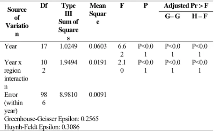
Results from repeated ANOVA and adjusted univariate analyses for within subject effects (year, region, and region by year interaction) are given in Table 4. Due to violation of spherity assumption, instead of repeated ANOVA, using adjusted significance value from G-G and H-F (Table 4) would be better. The results showed that null hypotheses of year and region by year interaction were rejected (Table 4) and interpreted that there is significant differences among years for wheat production. Significant “region by year interaction” term reflects that averages wheat production of regions varied significantly from year to year (Table 4).

2. Results of Multivariate Approaches in Repeated Measures Designs

2.1 Profile Analysis Results: Wheat productions of regions were changed significantly over years (Table 5). Accordingly, significant differences among average

values of wheat production amount of regions were clearly seen to be found (P<0.01).

Table 4. Results of within subjects effects Source of Variatio n Df Type III Sum of Square s Mean Squar e F P Adjusted Pr > F G– G H – F Year 17 1.0249 0.0603 6.6 2 P<0.0 1 P<0.0 1 P<0.0 1 Year x region interactio n 10 2 1.9494 0.0191 2.10 P<0.01 P<0.01 P<0.01 Error (within year) 98 6 8.9810 0.0091 Greenhouse-Geisser Epsilon: 0.2565 Huynh-Feldt Epsilon: 0.3086

Table 5. ANOVA table of combining years (coincident) Source of Variation Df Sum of Squares Mean Squares F P Between Regions 6 86.663 14.444 5.16 P<0.01 Error 58 162.267 2.798

Results regarding significance control of differences among years for wheat production are illustrated in Table 7. Probability values of four statistics used to test null hypothesis on year effect reflects significant differences among year levels (P<0.01).

Duncan’s Multiple comparison test results of regions’ wheat productions are given in Table 6. The differences between averages of Central Anatolia (with the highest wheat production) and the Eastern Anatolia, and between Central Anatolia and Blacksea regions were statistically significant (P<0.05).

Parallel test is equivalent to testing that there is no interaction of the within-subjects factor (year) with the between-subjects factor (region). When wheat production data were taken into consideration, parallel test is used to test whether the differences among years vary or not from region to region (Table 8). Thus, four statistics for testing parallel of profiles given in Table 8 demonstrated that, production profiles of regions were not parallel and differences among repeated measures varied from region to region (P<0.0001).

2.2. Results from Multivariate Approaches used in General Linear Model

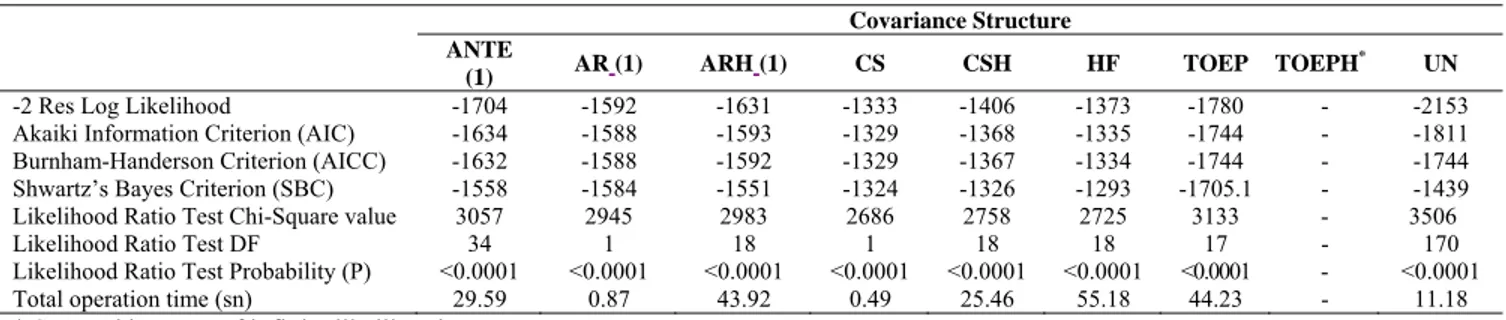
2.2.1. Containment approach: In general linear model, performances of models with different covariance structures in Containment approach, which is one of adjusted-df-approaches in repeated measures design are

given in Table 9. Compound symmetry (CS) was a covariance structure that has the best “goodness of fit” score in this approach. HF was the most suitable covariance structure after CS. However, covariance structure given the worst fit was unstructured (UN). No result for Heterogenous Toeplitz (TOEPH) was obtained because of infinite likelihood.

Table 6. Results of Duncan’s multiple comparison test regarding region averages

Region Province number Average

Central Anatolia 10 5.6108 a Mediterranean Sea 7 5.4521 a Southeast Anatolia 6 5.3499 ab Eastern Anatolia 12 4.8334 c Marmara 10 5.4156 a Aegean 8 5.2471 ab Black Sea 12 4.9882 bc

The values in calumn bearing different letters differ significant p<0.05.

Table 7. Flatness (between years) test results

Statistics Value F Num

sd Dem sd P Wilks' Lambda 0.10582 20.88 17 42 <0.0001 Pillai's Trace 0.89418 20.88 17 42 <0.0001 Hotelling L. Trace 8.45013 20.88 17 42 <0.0001 Roy's Gr. Root 8.45013 20.88 17 42 <0.0001

Rsults from Likelihood Ratio test (LRT) used to compare models including various covariance structures with the least square method are presented in Table 9. It was understood that models defined with eight different covariance structures in Containment approach gave better results than LS method.

Table 8. Parallel (Region by Year interaction) test results

Statistics Value F Numerator Df Deminator Df P Wilks' Lambda 0.02563 2.18 102 246.45 <.0001 Pillai's Trace 2.58208 2.09 102 282 <.0001 Hotelling L. Tr. 5.64492 2.24 102 156.29 <.0001 Roy's Gr. Root 2.12192 5.87 17 47 <.0001

Selection of the best covariance structure is essential for obtaining accurate results associated to fixed effects. Results of models (with several covariance structures) in respect of significance levels of fixed effects are given in Table 10. Region, year, and region by year interaction effects were significant for each covariance structure. Some differences in F values among covariances structures were determined (Table 10). In split plot design, using RANDOM command in MIXED procedure of SAS program with using CS in REPEATED line in GLM procedure gives similar results (Akbaş et al., 2001).

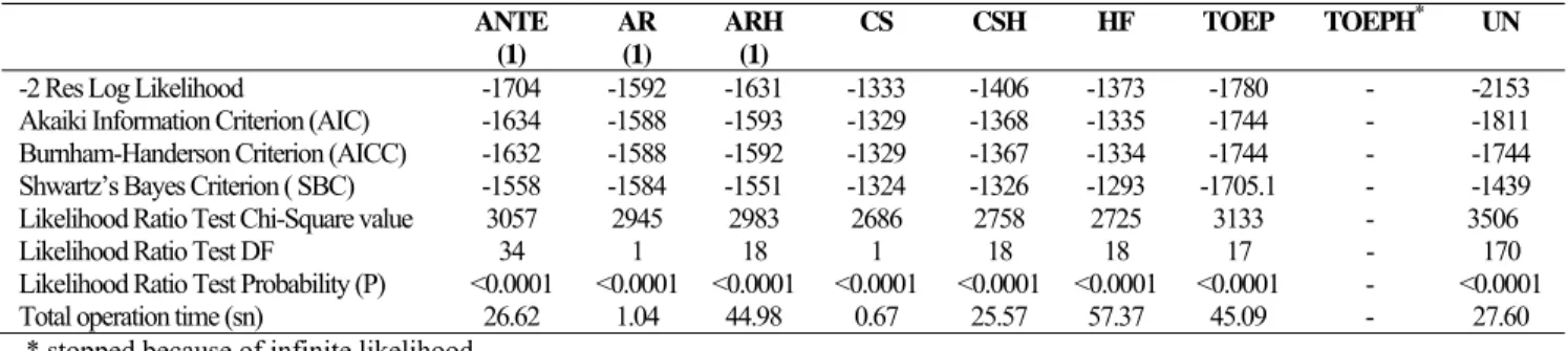
2.2.2. Satterthwaite approach: In general linear model, results of fitting performances of models with various Table 11. According to criteria in Table 11, the most appropriate covariance structure in Satterthwaite was Compound Symmetry that fitting values of criteria gave more closely to zero. The best three covariance structures were CS, HF, and CHS (Table 11).

Covariance structure Unstructured (UN) was the worst one for Satterthwaite approach. No result for

Table 9. Results of fit criteria used for comparing different covariance in Containment approach Covariance Structure

ANTE

(1) AR(1) ARH(1) CS CSH HF TOEP TOEPH

* _UN

-2 Res Log Likelihood -1704 -1592 -1631 -1333 -1406 -1373 -1780 - -2153

Akaiki Information Criterion (AIC) -1634 -1588 -1593 -1329 -1368 -1335 -1744 - -1811

Burnham-Handerson Criterion (AICC) -1632 -1588 -1592 -1329 -1367 -1334 -1744 - -1744

Shwartz’s Bayes Criterion (SBC) -1558 -1584 -1551 -1324 -1326 -1293 -1705.1 - -1439

Likelihood Ratio Test Chi-Square value 3057 2945 2983 2686 2758 2725 3133 - 3506

Likelihood Ratio Test DF 34 1 18 1 18 18 17 - 170

Likelihood Ratio Test Probability (P) <0.0001 <0.0001 <0.0001 <0.0001 <0.0001 <0.0001 <0.0001 - <0.0001

Total operation time (sn) 29.59 0.87 43.92 0.49 25.46 55.18 44.23 - 11.18

* Stopped because of infinite likelihood.

TOEPH was obtained. TOEPH gave a warning “stopped because of infinite likelihood” in MIXED prosedure of SAS program (Table 11). From Likelihood Ratio Test (LRT), it was determined that all models considered in Satterthwaite approach were more superior to LRT (Table 11).Fixed effects were significant (Table 12). For

HF covariance structure, region effect was only insignificant, whereas region, year and region by year interaction effects for other structures were significant at 1 % level.

2.2.3. Kenward-Roger approach: Fitting results of several covariance structures in Kenward Roger adjusted df approach are summarized in Table 13. In this approach, CS, HF, and CSH were the first three better covariance structures (Table 13).

There were no results for UN and TOEP structures in Kenward Roger approach.

AIC, AICC and SBC values of Containment, Satterthwaite and Kenward Roger adjusted-df-approaches were same under all circumstances. For each covariance structure, total operation times of Kenward Roger was longer time than those for other approaches. F values for fixed effects were found nearly similar in three multivariate approaches.

Table 10. Significance results of fixed effects in Containment approach (F and P values)

Covariance Structure

Region Year Region by Year

Interaction F P F P F P ANTE (1) 5.77 <0.0001 12.38 <0.0001 3.29 <0.0001 AR(1) 5.43 <0.0001 15.72 <0.0001 3.33 <0.0001 ARH(1) 5.03 <0.0001 14.61 <0.0001 3.35 <0.0001 CS 5.16 <0.0001 6.62 <0.0001 2.10 <0.0001 CSH 5.17 <0.0001 6.95 <0.0001 2.20 <0.0001 HF 2.41 0.0257 6.62 <0.0001 2.10 <0.0001 TOEP 4.96 <0.0001 12.79 <0.0001 2.99 <0.0001 TOEPH - - - - - - UN 5.16 <0.0001 28.83 <0.0001 3.21 <0.0001

Table 11. Results of fit criteria used for comparing different covariance in Satterhwaite approach ANTE (1) AR (1) ARH (1) CS CSH HF TOEP TOEPH* UN

-2 Res Log Likelihood -1704 -1592 -1631 -1333 -1406 -1373 -1780 - -2153 Akaiki Information Criterion (AIC) -1634 -1588 -1593 -1329 -1368 -1335 -1744 - -1811 Burnham-Handerson Criterion (AICC) -1632 -1588 -1592 -1329 -1367 -1334 -1744 - -1744 Shwartz’s Bayes Criterion ( SBC) -1558 -1584 -1551 -1324 -1326 -1293 -1705.1 - -1439 Likelihood Ratio Test Chi-Square value 3057 2945 2983 2686 2758 2725 3133 - 3506

Likelihood Ratio Test DF 34 1 18 1 18 18 17 - 170

Likelihood Ratio Test Probability (P) <0.0001 <0.0001 <0.0001 <0.0001 <0.0001 <0.0001 <0.0001 - <0.0001 Total operation time (sn) 26.62 1.04 44.98 0.67 25.57 57.37 45.09 - 27.60 * stopped because of infinite likelihood

Table 12. Significance results of fixed effects in Satterhwaite approach (F and P values)

Region Year Region by Year Interaction

Covariance Structure F P F P F P ANTE (1) 5.77 <0.0001 12.38 <0.0001 3.29 <0.0001 AR(1) 5.43 <0.0001 15.72 <0.0001 3.33 <0.0001 ARH(1) 5.03 0.0003 14.61 <0.0001 3.35 <0.0001 CS 5.16 0.0003 6.62 <0.0001 2.10 <0.0001 CSH 5.17 0.0003 6.95 <0.0001 2.20 <0.0001 HF 2.41 0.0838 6.62 <0.0001 2.10 <0.0001 TOEP 4.96 0.0004 12.79 <0.0001 2.99 <0.0001 TOEPH - - - - - - UN 5.16 0.0003 28.83 <0.0001 3.21 <0.0001

Table 13. Results of fit criteria used for comparing different covariance in Kenward-Roger approach

Covariance Structure

ANTE(1) AR(1) ARH(1) CS CSH HF TOEP TOEPH* UN** -2 Res Log Likelihood -1704 -1592 -1631 -1333 -1406 -1373 -1780 - - Akaiki Information Criterion (AIC) -1634 -1588 -1593 -1329 -1368 -1335 -1744 - - Burnham-Handerson Criterion

(AICC) -1632 -1588 -1592 -1329 -1367 -1334 -1744 - -

Shwartz’s Bayes Criterion ( SBC) -1558 -1584 -1551 -1325 -1326 -1293 -1705 - - Likelihood Ratio Test Chi-Square

value 3057 2945 2983 2686 2758 2725 3133 - -

Likelihood Ratio Test DF 34 1 18 1 18 18 17 - -

Likelihood Ratio Test Probability (P) <0.0001 <0.0001 <0.0001 <0.0001 <0.0001 <0.0001 <0.0001 - - Total operation time (sn) 1:33.48 1.46 1:01.67 1.09 43.89 1:16.62 1:00.32 - -

*Stopped because of infinite likelihood. ** Insufficient memory

Table 14. Significance results of fixed effects in Kenward Roger approach (F and P values)

Region Year Region by Year Interaction

Covariance Structure F P F P F P ANTE (1) 5.78 <0.0001 11.71 <0.0001 3.10 <0.0001 AR(1) 5.45 <0.0001 15.35 <0.0001 3.25 <0.0001 ARH(1) 5.03 0.0003 14.61 <0.0001 3.35 <0.0001 CS 5.16 0.0003 6.62 <0.0001 2.10 <0.0001 CSH 5.17 0.0003 6.72 <0.0001 2.12 <0.0001 HF 2.41 0.0838 6.62 <0.0001 2.10 <0.0001 TOEP 4.96 0.0004 12.29 <0.0001 2.86 <0.0001 TOEPH - - - UN - - -

DISCUSSION

This study was conducted to compare univariate and multivariate approaches in repeated measures designs. When Spherity assumption was violated in Repeated ANOVA, an univariate approach, it was examined to be taken measures. With using profile analysis, using several covariance structures in Containment, Satterthwaite, and Kenward Roger adjusted-df-approaches based on general linear model was also investigated.

In applications of univariate and multivariate approaches, F values calculated for fixed effects such as Region, Year, and Region by Year Interaction were statistically significant (P<0.001). That is, F values on within-subjects effects were statistically significant.

Split plot experimental design with two factors (between-subjects (region) and within-subjects effects (year)) has been used commonly in Repeated Measures Design. Repeated ANOVA is known as the simplest form of the experimental design with repeated measurement. When spherity assumption was violated according to mauchly statistic result (P<0.01) and evaluating results of fixed effects from Repeated ANOVA may be lead to faulty interpretations (Olson, 1974; Algina and Oshima, 1994; Tabachnichk and Fidel, 2001; Gürbüz et al., 2003; Eyduran et al., 2008).

For this reason; at the first stage, it was concluded that, the use of univariate approaches such as Greenhouse-Geisser Epsilon (G-G) and Huynh-Feldt Epsilon (H-F) or multivariate approaches for assessing within-subject effects would be more appropriate than that of Repeated ANOVA as in the current study. H-F has used more common than G-G, which shows more conservative form in determination of some real differences between-groups. In case of Spherity assumption violation, these two approaches provide Type I error ratio to stay limit values, reducing df (Box, 1954; Gürbüz et al., 2003; Keighley, 2005). However, in the event of ensured spherity assumption in Repeated ANOVA, power of test obtained from Repeated ANOVA

(univariate) was higher than that obtained from Multivariate Approach (Morrison, 1990; Movenon et al., 2007).

In Profile Analysis, known as Multivariate approach to Repeated Measures Design (Repeated MANOVA), F test results of Region, Year, and Region by Year interaction effects were also significant (P<0.01). It is desired that number of experimental unit (subjects) in each level of independent variable is higher than period number in Profile Analysis. Otherwise, power of test in Profile Analysis is reduced (Tabachnick and Fidell, 2001). Also, it was reported that the most ideal cases for Profile Analysis are i) balanced design and ii) unit number more than period number (Tabachnick and Fidell, 2001). Due to these reasons, instead of Profile Analysis, Mixed model methodology for current study data with repeated measurement was preferred. Because, number of experimental unit (6 to 12) was smaller than number of period number (18 year).

Mixed model methodolody in repeated measures design has more advantageous than Repeated ANOVA and Profile Analysis. Only mixed model was applied for data with / without missing observations and specified a variety of covariance structures for data with missing and no missing observations. Statistical analyses of data with missing observations are not executed for Repeated ANOVA and Profile Analysis (Littell et al., 1998).

According to results of Likelihood Ratio Test (LRT) for covariance structures in Containment, Satterhwaite and Kenward-Roger multivariate approaches, it was understood that models with these covariance structures provide better fit than least square approach. In simulation studies, even in the event of being small deviations on normal distribution and Spherity assumption, Keselman et al., (2003) reported that standard least square approach could not gave robust results. In another study carried out by Akbas et al., (2001), standard least square approach for general linear and general linear mixed models had lesser fit. It could be suggested that the findings on standard least square approach from the current study were in good agreement

with those of Akbas et al. (2001) and Keselman et al. (2003). Thus, it was understood that use of multivariate approaches in general linear model instead of standard least squares approach would more accurate.

Results obtained from the present study can be summarized below:

 In the event of violation of Spherity assumption, instead of Repeated ANOVA, Geisser-Greenhouse Epsilon, Huynh-Feldt Epsilon and multivariate (Containment, Satterthwaite and Kenward-Roger) approaches could be suggested. However, Containment, Satterthwaite and Kenward-Roger multivariate approaches allow researchers to define different covariances.

 It could be said that models including various covariances in Containment, Satterthwaite and Kenward-Roger multivariate approaches had better fit than standard least squares approach. Therefore, when Repeated ANOVA was insufficient, Containment, Satterthwaite and Kenward-Roger multivariate approaches should be used.

REFERENCES

Akaike, H. (1973). Information theory and an extension of the maximum likelihood principle. In Second International Symposium on Information Theory, B. N. Petrov and F. Csaki, eds. Akademiai Kiado, Budapest, 267-281.

Akbaş, Y., M. Z. Fırat and Ç. Yakupoğlu, (2001). Hayvancılıkta Tekrarlanan Ölçümlerin Analizinde Kullanılan Farklı Modellerin Karşılaştırılması ve SAS Uygulamaları. Tarımsal Bilişim Teknolojileri Sempozyumu, 20-22 Eylül 2001, Sütçü İmam Üniversitesi, Ziraat Fakültesi, Kahramanmaraş. Algina, J. and T. C. Oshima, (1994). Type I error rates for

Huynh’s General Approximation and Improved General Approximation tests. British J. Mathematical and Statistical Psychology, 47: 151-165.

Alpar, R. (2003). Uygulamalı Çok Değişkenli İstatistiksel Yöntemlere Giriş 1. Nobel Yayınları No: 452, ISBN: 975-591-431-5.

Barcikowski, R. S. and R. R. Robey (1984). Decision in single group repeated measures analysis: Statistical tests and three computer packages. The American Statistician, 38(2): 148-150.

Box, G. E. P. (1954). Some Theorems on Quadratic Forms Applied in the Study of Analysis of Variance Problems. II. Effects of Inequality of Variance and of Correlation between Errors in the Two-Way Classification. Annals of Mathematical Statistics, 25: 484-498.

Bozdoğan, H. (1987). Model selection and Akaike’s information criterion (AIC): the general theory and its analytical extensions. Psychometrika, 52: 345-370.

Eyduran, E., K. Yazgan and T. Özdemir, (2008). Utilization of Profile Analysis in Animal Science. J. of Anim. Vet. Advances, 7(7):796-798.

Gürbüz, F., E. Başpınar, H. Çamdeviren and S. Keskin, (2003). Tekrarlanan Ölçümlü Deneme Düzenlerinin Analizi. YYÜ. Matbaası, Van.130.

Hannan, E. J. and B. G. Quinn (1979). The determination of the order of an autoregression. J. Royal Statistical Society Series B, 41(2): 190-195.

Huynh, H. and L. S. Feldt (1970). Conditions under which mean square ratios in repeated measurements designs have exact F-distributions. J. American Statistical Association, 65(332): 1582-1589.

Keighley, J. D. (2005). A simulation study of power for a repeated measurements experiment using mixed model methodology (Ph.D thesis, unpublished). Kansas State University, Graduate School of the Kansas State University, Manhattan, Kansas.

Keselman, H. J., K. C. Carriere and L. M. Lix (1993). Testing repeated measures hypotheses when covariance matrices are heterogeneous. J. Educational Statistics, 18(4): 305-319.

Keselman, H. J., R. R. Wilcox and L. M. Lix, (2003). A Generally Robust Approach to Hypothesis Testing in Independent and Correlated Groups Designs. Psychophysiology. 40: 586-596.

Keskin, S., and M. Mendeş (2001). Faktörlerden birinin seviyelerinde tekrarlanan ölçüm bulunan iki faktörlü deneme düzenleri. S.Ü. Ziraat Fakültesi Dergisi, 15(25): 42-53.

Kowalchuk, R. K. (2000). Repeated Measures Multiple Comparison Prosedures with a mixel model Analysis (PhD. Thesis, unpublished). Manitoba University. Faculty of Graduate School of the Manitoba University, Manitoba.

Littell, R. C., G. A. Milliken, W. W. Stroup and R. D. Wolfinger, (1996), SAS System for Mixed Models, Cary, NC: SAS Institute Inc.

Looney, S. W., and W. B. Stanley, (1989). Exploratory repeated measures for two or more groups. The American Statistician, 43(4): 220-224.

Morrison, D. F. (1990). Multivariate statistical methods (3rd ed.). New York: McGraw-Hill.

Movenon, S.W., M. A. Betz, K. Wang and B. Zumbo, (2007). Application of a New Procedure for Power Analysis and Comparison of the Adjusted Univariate and Multivariate Tests in Repeated Measures Designs. J. Modern Applied Statistical Methods, 6(1):36-52.

Olson, C.L. (1974). Comparative robustness of Six tests in Multivariate Analysis of Variance. Journal of the American Statistical Association, 69: 894-908.

Schwarz, G. (1978). Estimating the dimension of a model, Annals of Statistics, 6: 461–464.

Tabachnick, B.G. and L. S. Fidel, (2001). Using Multivariate Statistics. Allyn& Bacon, USA.

TUİK, (1982). Türkiye İstatistik Kurumu. Tarım İstatistikleri Özeti. TUİK, (1999). Türkiye İstatistik Kurumu. Tarım İstatistikleri Özeti.